example hypothesis for correlational study

Have a language expert improve your writing

Run a free plagiarism check in 10 minutes, automatically generate references for free.

• Knowledge Base
• Methodology
• Correlational Research | Guide, Design & Examples

Correlational Research | Guide, Design & Examples

Published on 5 May 2022 by Pritha Bhandari . Revised on 5 December 2022.

A correlational research design investigates relationships between variables without the researcher controlling or manipulating any of them.

A correlation reflects the strength and/or direction of the relationship between two (or more) variables. The direction of a correlation can be either positive or negative.

Table of contents

Correlational vs experimental research, when to use correlational research, how to collect correlational data, how to analyse correlational data, correlation and causation, frequently asked questions about correlational research.

Correlational and experimental research both use quantitative methods to investigate relationships between variables. But there are important differences in how data is collected and the types of conclusions you can draw.

Prevent plagiarism, run a free check.

Correlational research is ideal for gathering data quickly from natural settings. That helps you generalise your findings to real-life situations in an externally valid way.

There are a few situations where correlational research is an appropriate choice.

To investigate non-causal relationships

You want to find out if there is an association between two variables, but you don’t expect to find a causal relationship between them.

Correlational research can provide insights into complex real-world relationships, helping researchers develop theories and make predictions.

To explore causal relationships between variables

You think there is a causal relationship between two variables, but it is impractical, unethical, or too costly to conduct experimental research that manipulates one of the variables.

Correlational research can provide initial indications or additional support for theories about causal relationships.

To test new measurement tools

You have developed a new instrument for measuring your variable, and you need to test its reliability or validity .

Correlational research can be used to assess whether a tool consistently or accurately captures the concept it aims to measure.

There are many different methods you can use in correlational research. In the social and behavioural sciences, the most common data collection methods for this type of research include surveys, observations, and secondary data.

It’s important to carefully choose and plan your methods to ensure the reliability and validity of your results. You should carefully select a representative sample so that your data reflects the population you’re interested in without bias .

In survey research , you can use questionnaires to measure your variables of interest. You can conduct surveys online, by post, by phone, or in person.

Surveys are a quick, flexible way to collect standardised data from many participants, but it’s important to ensure that your questions are worded in an unbiased way and capture relevant insights.

Naturalistic observation

Naturalistic observation is a type of field research where you gather data about a behaviour or phenomenon in its natural environment.

This method often involves recording, counting, describing, and categorising actions and events. Naturalistic observation can include both qualitative and quantitative elements, but to assess correlation, you collect data that can be analysed quantitatively (e.g., frequencies, durations, scales, and amounts).

Naturalistic observation lets you easily generalise your results to real-world contexts, and you can study experiences that aren’t replicable in lab settings. But data analysis can be time-consuming and unpredictable, and researcher bias may skew the interpretations.

Secondary data

Instead of collecting original data, you can also use data that has already been collected for a different purpose, such as official records, polls, or previous studies.

Using secondary data is inexpensive and fast, because data collection is complete. However, the data may be unreliable, incomplete, or not entirely relevant, and you have no control over the reliability or validity of the data collection procedures.

After collecting data, you can statistically analyse the relationship between variables using correlation or regression analyses, or both. You can also visualise the relationships between variables with a scatterplot.

Different types of correlation coefficients and regression analyses are appropriate for your data based on their levels of measurement and distributions .

Correlation analysis

Using a correlation analysis, you can summarise the relationship between variables into a correlation coefficient : a single number that describes the strength and direction of the relationship between variables. With this number, you’ll quantify the degree of the relationship between variables.

The Pearson product-moment correlation coefficient, also known as Pearson’s r , is commonly used for assessing a linear relationship between two quantitative variables.

Correlation coefficients are usually found for two variables at a time, but you can use a multiple correlation coefficient for three or more variables.

Regression analysis

With a regression analysis , you can predict how much a change in one variable will be associated with a change in the other variable. The result is a regression equation that describes the line on a graph of your variables.

You can use this equation to predict the value of one variable based on the given value(s) of the other variable(s). It’s best to perform a regression analysis after testing for a correlation between your variables.

It’s important to remember that correlation does not imply causation . Just because you find a correlation between two things doesn’t mean you can conclude one of them causes the other, for a few reasons.

Directionality problem

If two variables are correlated, it could be because one of them is a cause and the other is an effect. But the correlational research design doesn’t allow you to infer which is which. To err on the side of caution, researchers don’t conclude causality from correlational studies.

Third variable problem

A confounding variable is a third variable that influences other variables to make them seem causally related even though they are not. Instead, there are separate causal links between the confounder and each variable.

In correlational research, there’s limited or no researcher control over extraneous variables . Even if you statistically control for some potential confounders, there may still be other hidden variables that disguise the relationship between your study variables.

Although a correlational study can’t demonstrate causation on its own, it can help you develop a causal hypothesis that’s tested in controlled experiments.

A correlation reflects the strength and/or direction of the association between two or more variables.

• A positive correlation means that both variables change in the same direction.
• A negative correlation means that the variables change in opposite directions.
• A zero correlation means there’s no relationship between the variables.

A correlational research design investigates relationships between two variables (or more) without the researcher controlling or manipulating any of them. It’s a non-experimental type of quantitative research .

Controlled experiments establish causality, whereas correlational studies only show associations between variables.

• In an experimental design , you manipulate an independent variable and measure its effect on a dependent variable. Other variables are controlled so they can’t impact the results.
• In a correlational design , you measure variables without manipulating any of them. You can test whether your variables change together, but you can’t be sure that one variable caused a change in another.

In general, correlational research is high in external validity while experimental research is high in internal validity .

A correlation is usually tested for two variables at a time, but you can test correlations between three or more variables.

A correlation coefficient is a single number that describes the strength and direction of the relationship between your variables.

Different types of correlation coefficients might be appropriate for your data based on their levels of measurement and distributions . The Pearson product-moment correlation coefficient (Pearson’s r ) is commonly used to assess a linear relationship between two quantitative variables.

Cite this Scribbr article

If you want to cite this source, you can copy and paste the citation or click the ‘Cite this Scribbr article’ button to automatically add the citation to our free Reference Generator.

Bhandari, P. (2022, December 05). Correlational Research | Guide, Design & Examples. Scribbr. Retrieved 27 May 2024, from https://www.scribbr.co.uk/research-methods/correlational-research-design/

Is this article helpful?

Pritha Bhandari

Other students also liked, a quick guide to experimental design | 5 steps & examples, quasi-experimental design | definition, types & examples, qualitative vs quantitative research | examples & methods.

• school Campus Bookshelves
• menu_book Bookshelves
• perm_media Learning Objects
• login Login
• how_to_reg Request Instructor Account
• hub Instructor Commons

Margin Size

• Download Page (PDF)
• Download Full Book (PDF)
• Periodic Table
• Physics Constants
• Scientific Calculator
• Reference & Cite
• Tools expand_more
• Readability

selected template will load here

This action is not available.

11.2: Correlation Hypothesis Test

• Last updated
• Save as PDF
• Page ID 25691

\( \newcommand{\vecs}[1]{\overset { \scriptstyle \rightharpoonup} {\mathbf{#1}} } \)

\( \newcommand{\vecd}[1]{\overset{-\!-\!\rightharpoonup}{\vphantom{a}\smash {#1}}} \)

\( \newcommand{\id}{\mathrm{id}}\) \( \newcommand{\Span}{\mathrm{span}}\)

( \newcommand{\kernel}{\mathrm{null}\,}\) \( \newcommand{\range}{\mathrm{range}\,}\)

\( \newcommand{\RealPart}{\mathrm{Re}}\) \( \newcommand{\ImaginaryPart}{\mathrm{Im}}\)

\( \newcommand{\Argument}{\mathrm{Arg}}\) \( \newcommand{\norm}[1]{\| #1 \|}\)

\( \newcommand{\inner}[2]{\langle #1, #2 \rangle}\)

\( \newcommand{\Span}{\mathrm{span}}\)

\( \newcommand{\id}{\mathrm{id}}\)

\( \newcommand{\kernel}{\mathrm{null}\,}\)

\( \newcommand{\range}{\mathrm{range}\,}\)

\( \newcommand{\RealPart}{\mathrm{Re}}\)

\( \newcommand{\ImaginaryPart}{\mathrm{Im}}\)

\( \newcommand{\Argument}{\mathrm{Arg}}\)

\( \newcommand{\norm}[1]{\| #1 \|}\)

\( \newcommand{\Span}{\mathrm{span}}\) \( \newcommand{\AA}{\unicode[.8,0]{x212B}}\)

\( \newcommand{\vectorA}[1]{\vec{#1}}      % arrow\)

\( \newcommand{\vectorAt}[1]{\vec{\text{#1}}}      % arrow\)

\( \newcommand{\vectorB}[1]{\overset { \scriptstyle \rightharpoonup} {\mathbf{#1}} } \)

\( \newcommand{\vectorC}[1]{\textbf{#1}} \)

\( \newcommand{\vectorD}[1]{\overrightarrow{#1}} \)

\( \newcommand{\vectorDt}[1]{\overrightarrow{\text{#1}}} \)

\( \newcommand{\vectE}[1]{\overset{-\!-\!\rightharpoonup}{\vphantom{a}\smash{\mathbf {#1}}}} \)

The correlation coefficient, \(r\), tells us about the strength and direction of the linear relationship between \(x\) and \(y\). However, the reliability of the linear model also depends on how many observed data points are in the sample. We need to look at both the value of the correlation coefficient \(r\) and the sample size \(n\), together. We perform a hypothesis test of the "significance of the correlation coefficient" to decide whether the linear relationship in the sample data is strong enough to use to model the relationship in the population.

The sample data are used to compute \(r\), the correlation coefficient for the sample. If we had data for the entire population, we could find the population correlation coefficient. But because we have only sample data, we cannot calculate the population correlation coefficient. The sample correlation coefficient, \(r\), is our estimate of the unknown population correlation coefficient.

• The symbol for the population correlation coefficient is \(\rho\), the Greek letter "rho."
• \(\rho =\) population correlation coefficient (unknown)
• \(r =\) sample correlation coefficient (known; calculated from sample data)

The hypothesis test lets us decide whether the value of the population correlation coefficient \(\rho\) is "close to zero" or "significantly different from zero". We decide this based on the sample correlation coefficient \(r\) and the sample size \(n\).

If the test concludes that the correlation coefficient is significantly different from zero, we say that the correlation coefficient is "significant."

• Conclusion: There is sufficient evidence to conclude that there is a significant linear relationship between \(x\) and \(y\) because the correlation coefficient is significantly different from zero.
• What the conclusion means: There is a significant linear relationship between \(x\) and \(y\). We can use the regression line to model the linear relationship between \(x\) and \(y\) in the population.

If the test concludes that the correlation coefficient is not significantly different from zero (it is close to zero), we say that correlation coefficient is "not significant".

• Conclusion: "There is insufficient evidence to conclude that there is a significant linear relationship between \(x\) and \(y\) because the correlation coefficient is not significantly different from zero."
• What the conclusion means: There is not a significant linear relationship between \(x\) and \(y\). Therefore, we CANNOT use the regression line to model a linear relationship between \(x\) and \(y\) in the population.
• If \(r\) is significant and the scatter plot shows a linear trend, the line can be used to predict the value of \(y\) for values of \(x\) that are within the domain of observed \(x\) values.
• If \(r\) is not significant OR if the scatter plot does not show a linear trend, the line should not be used for prediction.
• If \(r\) is significant and if the scatter plot shows a linear trend, the line may NOT be appropriate or reliable for prediction OUTSIDE the domain of observed \(x\) values in the data.

PERFORMING THE HYPOTHESIS TEST

• Null Hypothesis: \(H_{0}: \rho = 0\)
• Alternate Hypothesis: \(H_{a}: \rho \neq 0\)

WHAT THE HYPOTHESES MEAN IN WORDS:

• Null Hypothesis \(H_{0}\) : The population correlation coefficient IS NOT significantly different from zero. There IS NOT a significant linear relationship(correlation) between \(x\) and \(y\) in the population.
• Alternate Hypothesis \(H_{a}\) : The population correlation coefficient IS significantly DIFFERENT FROM zero. There IS A SIGNIFICANT LINEAR RELATIONSHIP (correlation) between \(x\) and \(y\) in the population.

DRAWING A CONCLUSION:There are two methods of making the decision. The two methods are equivalent and give the same result.

• Method 1: Using the \(p\text{-value}\)
• Method 2: Using a table of critical values

In this chapter of this textbook, we will always use a significance level of 5%, \(\alpha = 0.05\)

Using the \(p\text{-value}\) method, you could choose any appropriate significance level you want; you are not limited to using \(\alpha = 0.05\). But the table of critical values provided in this textbook assumes that we are using a significance level of 5%, \(\alpha = 0.05\). (If we wanted to use a different significance level than 5% with the critical value method, we would need different tables of critical values that are not provided in this textbook.)

METHOD 1: Using a \(p\text{-value}\) to make a decision

Using the ti83, 83+, 84, 84+ calculator.

To calculate the \(p\text{-value}\) using LinRegTTEST:

On the LinRegTTEST input screen, on the line prompt for \(\beta\) or \(\rho\), highlight "\(\neq 0\)"

The output screen shows the \(p\text{-value}\) on the line that reads "\(p =\)".

(Most computer statistical software can calculate the \(p\text{-value}\).)

If the \(p\text{-value}\) is less than the significance level ( \(\alpha = 0.05\) ):

• Decision: Reject the null hypothesis.
• Conclusion: "There is sufficient evidence to conclude that there is a significant linear relationship between \(x\) and \(y\) because the correlation coefficient is significantly different from zero."

If the \(p\text{-value}\) is NOT less than the significance level ( \(\alpha = 0.05\) )

• Decision: DO NOT REJECT the null hypothesis.
• Conclusion: "There is insufficient evidence to conclude that there is a significant linear relationship between \(x\) and \(y\) because the correlation coefficient is NOT significantly different from zero."

Calculation Notes:

• You will use technology to calculate the \(p\text{-value}\). The following describes the calculations to compute the test statistics and the \(p\text{-value}\):
• The \(p\text{-value}\) is calculated using a \(t\)-distribution with \(n - 2\) degrees of freedom.
• The formula for the test statistic is \(t = \frac{r\sqrt{n-2}}{\sqrt{1-r^{2}}}\). The value of the test statistic, \(t\), is shown in the computer or calculator output along with the \(p\text{-value}\). The test statistic \(t\) has the same sign as the correlation coefficient \(r\).
• The \(p\text{-value}\) is the combined area in both tails.

An alternative way to calculate the \(p\text{-value}\) ( \(p\) ) given by LinRegTTest is the command 2*tcdf(abs(t),10^99, n-2) in 2nd DISTR.

THIRD-EXAM vs FINAL-EXAM EXAMPLE: \(p\text{-value}\) method

• Consider the third exam/final exam example.
• The line of best fit is: \(\hat{y} = -173.51 + 4.83x\) with \(r = 0.6631\) and there are \(n = 11\) data points.
• Can the regression line be used for prediction? Given a third exam score ( \(x\) value), can we use the line to predict the final exam score (predicted \(y\) value)?
• \(H_{0}: \rho = 0\)
• \(H_{a}: \rho \neq 0\)
• \(\alpha = 0.05\)
• The \(p\text{-value}\) is 0.026 (from LinRegTTest on your calculator or from computer software).
• The \(p\text{-value}\), 0.026, is less than the significance level of \(\alpha = 0.05\).
• Decision: Reject the Null Hypothesis \(H_{0}\)
• Conclusion: There is sufficient evidence to conclude that there is a significant linear relationship between the third exam score (\(x\)) and the final exam score (\(y\)) because the correlation coefficient is significantly different from zero.

Because \(r\) is significant and the scatter plot shows a linear trend, the regression line can be used to predict final exam scores.

METHOD 2: Using a table of Critical Values to make a decision

The 95% Critical Values of the Sample Correlation Coefficient Table can be used to give you a good idea of whether the computed value of \(r\) is significant or not . Compare \(r\) to the appropriate critical value in the table. If \(r\) is not between the positive and negative critical values, then the correlation coefficient is significant. If \(r\) is significant, then you may want to use the line for prediction.

Example \(\PageIndex{1}\)

Suppose you computed \(r = 0.801\) using \(n = 10\) data points. \(df = n - 2 = 10 - 2 = 8\). The critical values associated with \(df = 8\) are \(-0.632\) and \(+0.632\). If \(r <\) negative critical value or \(r >\) positive critical value, then \(r\) is significant. Since \(r = 0.801\) and \(0.801 > 0.632\), \(r\) is significant and the line may be used for prediction. If you view this example on a number line, it will help you.

Exercise \(\PageIndex{1}\)

For a given line of best fit, you computed that \(r = 0.6501\) using \(n = 12\) data points and the critical value is 0.576. Can the line be used for prediction? Why or why not?

If the scatter plot looks linear then, yes, the line can be used for prediction, because \(r >\) the positive critical value.

Example \(\PageIndex{2}\)

Suppose you computed \(r = –0.624\) with 14 data points. \(df = 14 – 2 = 12\). The critical values are \(-0.532\) and \(0.532\). Since \(-0.624 < -0.532\), \(r\) is significant and the line can be used for prediction

Exercise \(\PageIndex{2}\)

For a given line of best fit, you compute that \(r = 0.5204\) using \(n = 9\) data points, and the critical value is \(0.666\). Can the line be used for prediction? Why or why not?

No, the line cannot be used for prediction, because \(r <\) the positive critical value.

Example \(\PageIndex{3}\)

Suppose you computed \(r = 0.776\) and \(n = 6\). \(df = 6 - 2 = 4\). The critical values are \(-0.811\) and \(0.811\). Since \(-0.811 < 0.776 < 0.811\), \(r\) is not significant, and the line should not be used for prediction.

Exercise \(\PageIndex{3}\)

For a given line of best fit, you compute that \(r = -0.7204\) using \(n = 8\) data points, and the critical value is \(= 0.707\). Can the line be used for prediction? Why or why not?

Yes, the line can be used for prediction, because \(r <\) the negative critical value.

THIRD-EXAM vs FINAL-EXAM EXAMPLE: critical value method

Consider the third exam/final exam example. The line of best fit is: \(\hat{y} = -173.51 + 4.83x\) with \(r = 0.6631\) and there are \(n = 11\) data points. Can the regression line be used for prediction? Given a third-exam score ( \(x\) value), can we use the line to predict the final exam score (predicted \(y\) value)?

• Use the "95% Critical Value" table for \(r\) with \(df = n - 2 = 11 - 2 = 9\).
• The critical values are \(-0.602\) and \(+0.602\)
• Since \(0.6631 > 0.602\), \(r\) is significant.
• Conclusion:There is sufficient evidence to conclude that there is a significant linear relationship between the third exam score (\(x\)) and the final exam score (\(y\)) because the correlation coefficient is significantly different from zero.

Example \(\PageIndex{4}\)

Suppose you computed the following correlation coefficients. Using the table at the end of the chapter, determine if \(r\) is significant and the line of best fit associated with each r can be used to predict a \(y\) value. If it helps, draw a number line.

• \(r = –0.567\) and the sample size, \(n\), is \(19\). The \(df = n - 2 = 17\). The critical value is \(-0.456\). \(-0.567 < -0.456\) so \(r\) is significant.
• \(r = 0.708\) and the sample size, \(n\), is \(9\). The \(df = n - 2 = 7\). The critical value is \(0.666\). \(0.708 > 0.666\) so \(r\) is significant.
• \(r = 0.134\) and the sample size, \(n\), is \(14\). The \(df = 14 - 2 = 12\). The critical value is \(0.532\). \(0.134\) is between \(-0.532\) and \(0.532\) so \(r\) is not significant.
• \(r = 0\) and the sample size, \(n\), is five. No matter what the \(dfs\) are, \(r = 0\) is between the two critical values so \(r\) is not significant.

Exercise \(\PageIndex{4}\)

For a given line of best fit, you compute that \(r = 0\) using \(n = 100\) data points. Can the line be used for prediction? Why or why not?

No, the line cannot be used for prediction no matter what the sample size is.

Assumptions in Testing the Significance of the Correlation Coefficient

Testing the significance of the correlation coefficient requires that certain assumptions about the data are satisfied. The premise of this test is that the data are a sample of observed points taken from a larger population. We have not examined the entire population because it is not possible or feasible to do so. We are examining the sample to draw a conclusion about whether the linear relationship that we see between \(x\) and \(y\) in the sample data provides strong enough evidence so that we can conclude that there is a linear relationship between \(x\) and \(y\) in the population.

The regression line equation that we calculate from the sample data gives the best-fit line for our particular sample. We want to use this best-fit line for the sample as an estimate of the best-fit line for the population. Examining the scatter plot and testing the significance of the correlation coefficient helps us determine if it is appropriate to do this.

The assumptions underlying the test of significance are:

• There is a linear relationship in the population that models the average value of \(y\) for varying values of \(x\). In other words, the expected value of \(y\) for each particular value lies on a straight line in the population. (We do not know the equation for the line for the population. Our regression line from the sample is our best estimate of this line in the population.)
• The \(y\) values for any particular \(x\) value are normally distributed about the line. This implies that there are more \(y\) values scattered closer to the line than are scattered farther away. Assumption (1) implies that these normal distributions are centered on the line: the means of these normal distributions of \(y\) values lie on the line.
• The standard deviations of the population \(y\) values about the line are equal for each value of \(x\). In other words, each of these normal distributions of \(y\) values has the same shape and spread about the line.
• The residual errors are mutually independent (no pattern).
• The data are produced from a well-designed, random sample or randomized experiment.

Linear regression is a procedure for fitting a straight line of the form \(\hat{y} = a + bx\) to data. The conditions for regression are:

• Linear In the population, there is a linear relationship that models the average value of \(y\) for different values of \(x\).
• Independent The residuals are assumed to be independent.
• Normal The \(y\) values are distributed normally for any value of \(x\).
• Equal variance The standard deviation of the \(y\) values is equal for each \(x\) value.
• Random The data are produced from a well-designed random sample or randomized experiment.

The slope \(b\) and intercept \(a\) of the least-squares line estimate the slope \(\beta\) and intercept \(\alpha\) of the population (true) regression line. To estimate the population standard deviation of \(y\), \(\sigma\), use the standard deviation of the residuals, \(s\). \(s = \sqrt{\frac{SEE}{n-2}}\). The variable \(\rho\) (rho) is the population correlation coefficient. To test the null hypothesis \(H_{0}: \rho =\) hypothesized value , use a linear regression t-test. The most common null hypothesis is \(H_{0}: \rho = 0\) which indicates there is no linear relationship between \(x\) and \(y\) in the population. The TI-83, 83+, 84, 84+ calculator function LinRegTTest can perform this test (STATS TESTS LinRegTTest).

Formula Review

Least Squares Line or Line of Best Fit:

\[\hat{y} = a + bx\]

\[a = y\text{-intercept}\]

\[b = \text{slope}\]

Standard deviation of the residuals:

\[s = \sqrt{\frac{SSE}{n-2}}\]

\[SSE = \text{sum of squared errors}\]

\[n = \text{the number of data points}\]

Want to create or adapt books like this? Learn more about how Pressbooks supports open publishing practices.

7.2 Correlational Research

Learning objectives.

• Define correlational research and give several examples.
• Explain why a researcher might choose to conduct correlational research rather than experimental research or another type of nonexperimental research.

What Is Correlational Research?

Correlational research is a type of nonexperimental research in which the researcher measures two variables and assesses the statistical relationship (i.e., the correlation) between them with little or no effort to control extraneous variables. There are essentially two reasons that researchers interested in statistical relationships between variables would choose to conduct a correlational study rather than an experiment. The first is that they do not believe that the statistical relationship is a causal one. For example, a researcher might evaluate the validity of a brief extraversion test by administering it to a large group of participants along with a longer extraversion test that has already been shown to be valid. This researcher might then check to see whether participants’ scores on the brief test are strongly correlated with their scores on the longer one. Neither test score is thought to cause the other, so there is no independent variable to manipulate. In fact, the terms independent variable and dependent variable do not apply to this kind of research.

The other reason that researchers would choose to use a correlational study rather than an experiment is that the statistical relationship of interest is thought to be causal, but the researcher cannot manipulate the independent variable because it is impossible, impractical, or unethical. For example, Allen Kanner and his colleagues thought that the number of “daily hassles” (e.g., rude salespeople, heavy traffic) that people experience affects the number of physical and psychological symptoms they have (Kanner, Coyne, Schaefer, & Lazarus, 1981). But because they could not manipulate the number of daily hassles their participants experienced, they had to settle for measuring the number of daily hassles—along with the number of symptoms—using self-report questionnaires. Although the strong positive relationship they found between these two variables is consistent with their idea that hassles cause symptoms, it is also consistent with the idea that symptoms cause hassles or that some third variable (e.g., neuroticism) causes both.

A common misconception among beginning researchers is that correlational research must involve two quantitative variables, such as scores on two extraversion tests or the number of hassles and number of symptoms people have experienced. However, the defining feature of correlational research is that the two variables are measured—neither one is manipulated—and this is true regardless of whether the variables are quantitative or categorical. Imagine, for example, that a researcher administers the Rosenberg Self-Esteem Scale to 50 American college students and 50 Japanese college students. Although this “feels” like a between-subjects experiment, it is a correlational study because the researcher did not manipulate the students’ nationalities. The same is true of the study by Cacioppo and Petty comparing college faculty and factory workers in terms of their need for cognition. It is a correlational study because the researchers did not manipulate the participants’ occupations.

Figure 7.2 “Results of a Hypothetical Study on Whether People Who Make Daily To-Do Lists Experience Less Stress Than People Who Do Not Make Such Lists” shows data from a hypothetical study on the relationship between whether people make a daily list of things to do (a “to-do list”) and stress. Notice that it is unclear whether this is an experiment or a correlational study because it is unclear whether the independent variable was manipulated. If the researcher randomly assigned some participants to make daily to-do lists and others not to, then it is an experiment. If the researcher simply asked participants whether they made daily to-do lists, then it is a correlational study. The distinction is important because if the study was an experiment, then it could be concluded that making the daily to-do lists reduced participants’ stress. But if it was a correlational study, it could only be concluded that these variables are statistically related. Perhaps being stressed has a negative effect on people’s ability to plan ahead (the directionality problem). Or perhaps people who are more conscientious are more likely to make to-do lists and less likely to be stressed (the third-variable problem). The crucial point is that what defines a study as experimental or correlational is not the variables being studied, nor whether the variables are quantitative or categorical, nor the type of graph or statistics used to analyze the data. It is how the study is conducted.

Figure 7.2 Results of a Hypothetical Study on Whether People Who Make Daily To-Do Lists Experience Less Stress Than People Who Do Not Make Such Lists

Data Collection in Correlational Research

Again, the defining feature of correlational research is that neither variable is manipulated. It does not matter how or where the variables are measured. A researcher could have participants come to a laboratory to complete a computerized backward digit span task and a computerized risky decision-making task and then assess the relationship between participants’ scores on the two tasks. Or a researcher could go to a shopping mall to ask people about their attitudes toward the environment and their shopping habits and then assess the relationship between these two variables. Both of these studies would be correlational because no independent variable is manipulated. However, because some approaches to data collection are strongly associated with correlational research, it makes sense to discuss them here. The two we will focus on are naturalistic observation and archival data. A third, survey research, is discussed in its own chapter.

Naturalistic Observation

Naturalistic observation is an approach to data collection that involves observing people’s behavior in the environment in which it typically occurs. Thus naturalistic observation is a type of field research (as opposed to a type of laboratory research). It could involve observing shoppers in a grocery store, children on a school playground, or psychiatric inpatients in their wards. Researchers engaged in naturalistic observation usually make their observations as unobtrusively as possible so that participants are often not aware that they are being studied. Ethically, this is considered to be acceptable if the participants remain anonymous and the behavior occurs in a public setting where people would not normally have an expectation of privacy. Grocery shoppers putting items into their shopping carts, for example, are engaged in public behavior that is easily observable by store employees and other shoppers. For this reason, most researchers would consider it ethically acceptable to observe them for a study. On the other hand, one of the arguments against the ethicality of the naturalistic observation of “bathroom behavior” discussed earlier in the book is that people have a reasonable expectation of privacy even in a public restroom and that this expectation was violated.

Researchers Robert Levine and Ara Norenzayan used naturalistic observation to study differences in the “pace of life” across countries (Levine & Norenzayan, 1999). One of their measures involved observing pedestrians in a large city to see how long it took them to walk 60 feet. They found that people in some countries walked reliably faster than people in other countries. For example, people in the United States and Japan covered 60 feet in about 12 seconds on average, while people in Brazil and Romania took close to 17 seconds.

Because naturalistic observation takes place in the complex and even chaotic “real world,” there are two closely related issues that researchers must deal with before collecting data. The first is sampling. When, where, and under what conditions will the observations be made, and who exactly will be observed? Levine and Norenzayan described their sampling process as follows:

Male and female walking speed over a distance of 60 feet was measured in at least two locations in main downtown areas in each city. Measurements were taken during main business hours on clear summer days. All locations were flat, unobstructed, had broad sidewalks, and were sufficiently uncrowded to allow pedestrians to move at potentially maximum speeds. To control for the effects of socializing, only pedestrians walking alone were used. Children, individuals with obvious physical handicaps, and window-shoppers were not timed. Thirty-five men and 35 women were timed in most cities. (p. 186)

Precise specification of the sampling process in this way makes data collection manageable for the observers, and it also provides some control over important extraneous variables. For example, by making their observations on clear summer days in all countries, Levine and Norenzayan controlled for effects of the weather on people’s walking speeds.

The second issue is measurement. What specific behaviors will be observed? In Levine and Norenzayan’s study, measurement was relatively straightforward. They simply measured out a 60-foot distance along a city sidewalk and then used a stopwatch to time participants as they walked over that distance. Often, however, the behaviors of interest are not so obvious or objective. For example, researchers Robert Kraut and Robert Johnston wanted to study bowlers’ reactions to their shots, both when they were facing the pins and then when they turned toward their companions (Kraut & Johnston, 1979). But what “reactions” should they observe? Based on previous research and their own pilot testing, Kraut and Johnston created a list of reactions that included “closed smile,” “open smile,” “laugh,” “neutral face,” “look down,” “look away,” and “face cover” (covering one’s face with one’s hands). The observers committed this list to memory and then practiced by coding the reactions of bowlers who had been videotaped. During the actual study, the observers spoke into an audio recorder, describing the reactions they observed. Among the most interesting results of this study was that bowlers rarely smiled while they still faced the pins. They were much more likely to smile after they turned toward their companions, suggesting that smiling is not purely an expression of happiness but also a form of social communication.

Naturalistic observation has revealed that bowlers tend to smile when they turn away from the pins and toward their companions, suggesting that smiling is not purely an expression of happiness but also a form of social communication.

sieneke toering – bowling big lebowski style – CC BY-NC-ND 2.0.

When the observations require a judgment on the part of the observers—as in Kraut and Johnston’s study—this process is often described as coding . Coding generally requires clearly defining a set of target behaviors. The observers then categorize participants individually in terms of which behavior they have engaged in and the number of times they engaged in each behavior. The observers might even record the duration of each behavior. The target behaviors must be defined in such a way that different observers code them in the same way. This is the issue of interrater reliability. Researchers are expected to demonstrate the interrater reliability of their coding procedure by having multiple raters code the same behaviors independently and then showing that the different observers are in close agreement. Kraut and Johnston, for example, video recorded a subset of their participants’ reactions and had two observers independently code them. The two observers showed that they agreed on the reactions that were exhibited 97% of the time, indicating good interrater reliability.

Archival Data

Another approach to correlational research is the use of archival data , which are data that have already been collected for some other purpose. An example is a study by Brett Pelham and his colleagues on “implicit egotism”—the tendency for people to prefer people, places, and things that are similar to themselves (Pelham, Carvallo, & Jones, 2005). In one study, they examined Social Security records to show that women with the names Virginia, Georgia, Louise, and Florence were especially likely to have moved to the states of Virginia, Georgia, Louisiana, and Florida, respectively.

As with naturalistic observation, measurement can be more or less straightforward when working with archival data. For example, counting the number of people named Virginia who live in various states based on Social Security records is relatively straightforward. But consider a study by Christopher Peterson and his colleagues on the relationship between optimism and health using data that had been collected many years before for a study on adult development (Peterson, Seligman, & Vaillant, 1988). In the 1940s, healthy male college students had completed an open-ended questionnaire about difficult wartime experiences. In the late 1980s, Peterson and his colleagues reviewed the men’s questionnaire responses to obtain a measure of explanatory style—their habitual ways of explaining bad events that happen to them. More pessimistic people tend to blame themselves and expect long-term negative consequences that affect many aspects of their lives, while more optimistic people tend to blame outside forces and expect limited negative consequences. To obtain a measure of explanatory style for each participant, the researchers used a procedure in which all negative events mentioned in the questionnaire responses, and any causal explanations for them, were identified and written on index cards. These were given to a separate group of raters who rated each explanation in terms of three separate dimensions of optimism-pessimism. These ratings were then averaged to produce an explanatory style score for each participant. The researchers then assessed the statistical relationship between the men’s explanatory style as college students and archival measures of their health at approximately 60 years of age. The primary result was that the more optimistic the men were as college students, the healthier they were as older men. Pearson’s r was +.25.

This is an example of content analysis —a family of systematic approaches to measurement using complex archival data. Just as naturalistic observation requires specifying the behaviors of interest and then noting them as they occur, content analysis requires specifying keywords, phrases, or ideas and then finding all occurrences of them in the data. These occurrences can then be counted, timed (e.g., the amount of time devoted to entertainment topics on the nightly news show), or analyzed in a variety of other ways.

Key Takeaways

• Correlational research involves measuring two variables and assessing the relationship between them, with no manipulation of an independent variable.
• Correlational research is not defined by where or how the data are collected. However, some approaches to data collection are strongly associated with correlational research. These include naturalistic observation (in which researchers observe people’s behavior in the context in which it normally occurs) and the use of archival data that were already collected for some other purpose.

Discussion: For each of the following, decide whether it is most likely that the study described is experimental or correlational and explain why.

• An educational researcher compares the academic performance of students from the “rich” side of town with that of students from the “poor” side of town.
• A cognitive psychologist compares the ability of people to recall words that they were instructed to “read” with their ability to recall words that they were instructed to “imagine.”
• A manager studies the correlation between new employees’ college grade point averages and their first-year performance reports.
• An automotive engineer installs different stick shifts in a new car prototype, each time asking several people to rate how comfortable the stick shift feels.
• A food scientist studies the relationship between the temperature inside people’s refrigerators and the amount of bacteria on their food.
• A social psychologist tells some research participants that they need to hurry over to the next building to complete a study. She tells others that they can take their time. Then she observes whether they stop to help a research assistant who is pretending to be hurt.

Kanner, A. D., Coyne, J. C., Schaefer, C., & Lazarus, R. S. (1981). Comparison of two modes of stress measurement: Daily hassles and uplifts versus major life events. Journal of Behavioral Medicine, 4 , 1–39.

Kraut, R. E., & Johnston, R. E. (1979). Social and emotional messages of smiling: An ethological approach. Journal of Personality and Social Psychology, 37 , 1539–1553.

Levine, R. V., & Norenzayan, A. (1999). The pace of life in 31 countries. Journal of Cross-Cultural Psychology, 30 , 178–205.

Pelham, B. W., Carvallo, M., & Jones, J. T. (2005). Implicit egotism. Current Directions in Psychological Science, 14 , 106–110.

Peterson, C., Seligman, M. E. P., & Vaillant, G. E. (1988). Pessimistic explanatory style is a risk factor for physical illness: A thirty-five year longitudinal study. Journal of Personality and Social Psychology, 55 , 23–27.

Research Methods in Psychology Copyright © 2016 by University of Minnesota is licensed under a Creative Commons Attribution-NonCommercial-ShareAlike 4.0 International License , except where otherwise noted.

User Preferences

Content preview.

Arcu felis bibendum ut tristique et egestas quis:

• Ut enim ad minim veniam, quis nostrud exercitation ullamco laboris
• Duis aute irure dolor in reprehenderit in voluptate
• Excepteur sint occaecat cupidatat non proident

Keyboard Shortcuts

1.9 - hypothesis test for the population correlation coefficient.

There is one more point we haven't stressed yet in our discussion about the correlation coefficient r and the coefficient of determination \(R^{2}\) — namely, the two measures summarize the strength of a linear relationship in samples only . If we obtained a different sample, we would obtain different correlations, different \(R^{2}\) values, and therefore potentially different conclusions. As always, we want to draw conclusions about populations , not just samples. To do so, we either have to conduct a hypothesis test or calculate a confidence interval. In this section, we learn how to conduct a hypothesis test for the population correlation coefficient \(\rho\) (the greek letter "rho").

In general, a researcher should use the hypothesis test for the population correlation \(\rho\) to learn of a linear association between two variables, when it isn't obvious which variable should be regarded as the response. Let's clarify this point with examples of two different research questions.

Consider evaluating whether or not a linear relationship exists between skin cancer mortality and latitude. We will see in Lesson 2 that we can perform either of the following tests:

• t -test for testing \(H_{0} \colon \beta_{1}= 0\)
• ANOVA F -test for testing \(H_{0} \colon \beta_{1}= 0\)

For this example, it is fairly obvious that latitude should be treated as the predictor variable and skin cancer mortality as the response.

By contrast, suppose we want to evaluate whether or not a linear relationship exists between a husband's age and his wife's age ( Husband and Wife data ). In this case, one could treat the husband's age as the response:

...or one could treat the wife's age as the response:

In cases such as these, we answer our research question concerning the existence of a linear relationship by using the t -test for testing the population correlation coefficient \(H_{0}\colon \rho = 0\).

Let's jump right to it! We follow standard hypothesis test procedures in conducting a hypothesis test for the population correlation coefficient \(\rho\).

Steps for Hypothesis Testing for \(\boldsymbol{\rho}\) Section  

Step 1: hypotheses.

First, we specify the null and alternative hypotheses:

• Null hypothesis \(H_{0} \colon \rho = 0\)
• Alternative hypothesis \(H_{A} \colon \rho ≠ 0\) or \(H_{A} \colon \rho < 0\) or \(H_{A} \colon \rho > 0\)

Step 2: Test Statistic

Second, we calculate the value of the test statistic using the following formula:

Test statistic:  \(t^*=\dfrac{r\sqrt{n-2}}{\sqrt{1-R^2}}\) 

Step 3: P-Value

Third, we use the resulting test statistic to calculate the P -value. As always, the P -value is the answer to the question "how likely is it that we’d get a test statistic t* as extreme as we did if the null hypothesis were true?" The P -value is determined by referring to a t- distribution with n -2 degrees of freedom.

Step 4: Decision

Finally, we make a decision:

• If the P -value is smaller than the significance level \(\alpha\), we reject the null hypothesis in favor of the alternative. We conclude that "there is sufficient evidence at the\(\alpha\) level to conclude that there is a linear relationship in the population between the predictor x and response y."
• If the P -value is larger than the significance level \(\alpha\), we fail to reject the null hypothesis. We conclude "there is not enough evidence at the  \(\alpha\) level to conclude that there is a linear relationship in the population between the predictor x and response y ."

Example 1-5: Husband and Wife Data Section  

Let's perform the hypothesis test on the husband's age and wife's age data in which the sample correlation based on n = 170 couples is r = 0.939. To test \(H_{0} \colon \rho = 0\) against the alternative \(H_{A} \colon \rho ≠ 0\), we obtain the following test statistic:

\begin{align} t^*&=\dfrac{r\sqrt{n-2}}{\sqrt{1-R^2}}\\ &=\dfrac{0.939\sqrt{170-2}}{\sqrt{1-0.939^2}}\\ &=35.39\end{align}

To obtain the P -value, we need to compare the test statistic to a t -distribution with 168 degrees of freedom (since 170 - 2 = 168). In particular, we need to find the probability that we'd observe a test statistic more extreme than 35.39, and then, since we're conducting a two-sided test, multiply the probability by 2. Minitab helps us out here:

Student's t distribution with 168 DF

The output tells us that the probability of getting a test-statistic smaller than 35.39 is greater than 0.999. Therefore, the probability of getting a test-statistic greater than 35.39 is less than 0.001. As illustrated in the following video, we multiply by 2 and determine that the P-value is less than 0.002.

Since the P -value is small — smaller than 0.05, say — we can reject the null hypothesis. There is sufficient statistical evidence at the \(\alpha = 0.05\) level to conclude that there is a significant linear relationship between a husband's age and his wife's age.

Incidentally, we can let statistical software like Minitab do all of the dirty work for us. In doing so, Minitab reports:

Correlation: WAge, HAge

Pearson correlation of WAge and HAge = 0.939

P-Value = 0.000

Final Note Section  

One final note ... as always, we should clarify when it is okay to use the t -test for testing \(H_{0} \colon \rho = 0\)? The guidelines are a straightforward extension of the "LINE" assumptions made for the simple linear regression model. It's okay:

• When it is not obvious which variable is the response.
• For each x , the y 's are normal with equal variances.
• For each y , the x 's are normal with equal variances.
• Either, y can be considered a linear function of x .
• Or, x can be considered a linear function of y .
• The ( x , y ) pairs are independent

Our websites may use cookies to personalize and enhance your experience. By continuing without changing your cookie settings, you agree to this collection. For more information, please see our University Websites Privacy Notice .

Neag School of Education

Educational Research Basics by Del Siegle

Introduction to correlation research.

The PowerPoint presentation contains important information for this unit on correlations. Contact the instructor, [email protected] …if you have trouble viewing it.

Some content on this website may require the use of a plug-in, such as Microsoft PowerPoint .

When are correlation methods used?

• They are used to determine the extent to which two or more variables are related among a single group of people (although sometimes each pair of score does not come from one person…the correlation between father’s and son’s height would not).
• There is no attempt to manipulate the variables (random variables)

How is correlational research different from experimental research? In correlational research we do not (or at least try not to) influence any variables but only measure them and look for relations (correlations) between some set of variables, such as blood pressure and cholesterol level. In experimental research, we manipulate some variables and then measure the effects of this manipulation on other variables; for example, a researcher might artificially increase blood pressure and then record cholesterol level. Data analysis in experimental research also comes down to calculating “correlations” between variables, specifically, those manipulated and those affected by the manipulation. However, experimental data may potentially provide qualitatively better information: Only experimental data can conclusively demonstrate causal relations between variables. For example, if we found that whenever we change variable A then variable B changes, then we can conclude that “A influences B.” Data from correlational research can only be “interpreted” in causal terms based on some theories that we have, but correlational data cannot conclusively prove causality. Source: http://www.statsoft.com/textbook/stathome.html

Although a relationship between two variables does not prove that one caused the other, if there is no relationship between two variables then one cannot have caused the other.

Correlation research asks the question: What relationship exists?

• A correlation has direction and can be either positive or negative (note exceptions listed later). With a positive correlation, individuals who score above (or below) the average (mean) on one measure tend to score similarly above (or below) the average on the other measure.  The scatterplot of a positive correlation rises (from left to right). With negative relationships, an individual who scores above average on one measure tends to score below average on the other (or vise verse). The scatterplot of a negative correlation falls (from left to right).
• A correlation can differ in the degree or strength of the relationship (with the Pearson product-moment correlation coefficient that relationship is linear). Zero indicates no relationship between the two measures and r = 1.00 or r = -1.00 indicates a perfect relationship. The strength can be anywhere between 0 and + 1.00.  Note:  The symbol r is used to represent the Pearson product-moment correlation coefficient for a sample.  The Greek letter rho ( r ) is used for a population. The stronger the correlation–the closer the value of r (correlation coefficient) comes to + 1.00–the more the scatterplot will plot along a line.

When there is no relationship between the measures (variables), we say they are unrelated, uncorrelated, orthogonal, or independent .

Some Math for Bivariate Product Moment Correlation (not required for EPSY 5601): Multiple the z scores of each pair and add all of those products. Divide that by one less than the number of pairs of scores. (pretty easy)

Rather than calculating the correlation coefficient with either of the formulas shown above, you can simply follow these linked directions for using the function built into Microsoft’s Excel .

Some correlation questions elementary students can investigate are What is the relationship between…

• school attendance and grades in school?
• hours spend each week doing homework and school grades?
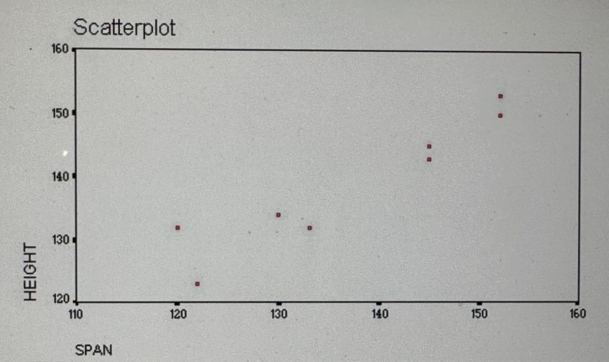
• length of arm span and height?
• number of children in a family and the number of bedrooms in the house?

Correlations only describe the relationship, they do not prove cause and effect. Correlation is a necessary, but not a sufficient condition for determining causality.

There are Three Requirements to Infer a Causal Relationship

• A statistically significant relationship between the variables
• The causal variable occurred prior to the other variable
• There are no other factors that could account for the cause

(Correlation studies do not meet the last requirement and may not meet the second requirement. However, not having a relationship does mean that one variable did not cause the other.)

There is a strong relationship between the number of ice cream cones sold and the number of people who drown each month.  Just because there is a relationship (strong correlation) does not mean that one caused the other.

If there is a relationship between A (ice cream cone sales) and B (drowning) it could be because

• A->B (Eating ice cream causes drowning)
• A<-B (Drowning cause people to eat ice cream– perhaps the mourners are so upset that they buy ice cream cones to cheer themselves)
• A<-C->B (Something else is related to both ice cream sales and the number of drowning– warm weather would be a good guess)

The points is…just because there is a correlation, you CANNOT say that the one variable causes the other.  On the other hand, if there is NO correlations, you can say that one DID NOT cause the other (assuming the measures are valid and reliable).

Format for correlations research questions and hypotheses:

Question: Is there a (statistically significant) relationship between height and arm span? H O : There is no (statistically significant) relationship between height and arm span (H 0 : r =0). H A : There is a (statistically significant) relationship between height and arm span (H A : r <>0).

Coefficient of Determination (Shared Variation)

One way researchers often express the strength of the relationship between two variables is by squaring their correlation coefficient. This squared correlation coefficient is called a COEFFICIENT OF DETERMINATION. The coefficient of determination is useful because it gives the proportion of the variance of one variable that is predictable from the other variable.

Factors which could limit a product-moment correlation coefficient ( PowerPoint demonstrating these factors )

• Homogenous group (the subjects are very similar on the variables)
• Unreliable measurement instrument (your measurements can’t be trusted and bounce all over the place)
• Nonlinear relationship (Pearson’s r is based on linear relationships…other formulas can be used in this case)
• Ceiling or Floor with measurement (lots of scores clumped at the top or bottom…therefore no spread which creates a problem similar to the homogeneous group)

Assumptions one must meet in order to use the Pearson product-moment correlation

• The measures are approximately normally distributed
• The variance of the two measures is similar ( homoscedasticity ) — check with scatterplot
• The relationship is linear — check with scatterplot
• The sample represents the population
• The variables are measured on a interval or ratio scale

There are different types of relationships: Linear – Nonlinear or Curvilinear – Non-monotonic (concave or cyclical). Different procedures are used to measure different types of relationships using different types of scales . The issue of measurement  scales   is very important for this class.  Be sure that you understand them.

Predictor and Criterion Variables (NOT NEEDED FOR EPSY 5601)

• Multiple Correlation- lots of predictors and one criterion ( R )
• Partial Correlation- correlation of two variables after their correlation with other variables is removed
• Serial or Autocorrelation- correlation of a set of number with itself (only staggered one)
• Canonical Correlation- lots of predictors and lots of criterion R c

When using a critical value table for Pearson’s product-moment correlation , the value found through the intersection of degree of freedom ( n – 2) and the alpha level you are testing ( p = .05) is the minimum r value needed in order for the relationship to be above chance alone.

The statistics package SPSS as well as Microsoft’s Excel can be used to calculate the correlation.

We will use Microsoft’s Excel .

Reading a Correlations Table in a Journal Article

Most research studies report the correlations among a set of variables. The results are presented in a table such as the one shown below.

The intersection of a row and column shows the correlation between the variable listed for the row and the variable listed for the column. For example, the intersection of the row mathematics and the column science shows that the correlation between mathematics and science was .874. The footnote states that the three *** after .874 indicate the relationship was statistically significant at p <.001.

Most tables do not report the perfect correlation along the diagonal that occurs when a variable is correlated with itself. In the example above, the diagonal was used to report the correlation of the four factors with a different variable. Because the correlation between reading and mathematics can be determined in the top section of the table, the correlations between those two variables is not repeated in the bottom half of the table. This is true for all of the relationships reported in the table.  .

Del Siegle, Ph.D. Neag School of Education – University of Connecticut [email protected] www.delsiegle.com

Last updated 10/11/2015

6.2 Correlational Research

Learning objectives.

• Define correlational research and give several examples.
• Explain why a researcher might choose to conduct correlational research rather than experimental research or another type of non-experimental research.
• Interpret the strength and direction of different correlation coefficients.
• Explain why correlation does not imply causation.

What Is Correlational Research?

Correlational research is a type of non-experimental research in which the researcher measures two variables and assesses the statistical relationship (i.e., the correlation) between them with little or no effort to control extraneous variables. There are many reasons that researchers interested in statistical relationships between variables would choose to conduct a correlational study rather than an experiment. The first is that they do not believe that the statistical relationship is a causal one or are not interested in causal relationships. Recall two goals of science are to describe and to predict and the correlational research strategy allows researchers to achieve both of these goals. Specifically, this strategy can be used to describe the strength and direction of the relationship between two variables and if there is a relationship between the variables then the researchers can use scores on one variable to predict scores on the other (using a statistical technique called regression).

Another reason that researchers would choose to use a correlational study rather than an experiment is that the statistical relationship of interest is thought to be causal, but the researcher  cannot  manipulate the independent variable because it is impossible, impractical, or unethical. For example, while I might be interested in the relationship between the frequency people use cannabis and their memory abilities I cannot ethically manipulate the frequency that people use cannabis. As such, I must rely on the correlational research strategy; I must simply measure the frequency that people use cannabis and measure their memory abilities using a standardized test of memory and then determine whether the frequency people use cannabis use is statistically related to memory test performance. 

Correlation is also used to establish the reliability and validity of measurements. For example, a researcher might evaluate the validity of a brief extraversion test by administering it to a large group of participants along with a longer extraversion test that has already been shown to be valid. This researcher might then check to see whether participants’ scores on the brief test are strongly correlated with their scores on the longer one. Neither test score is thought to cause the other, so there is no independent variable to manipulate. In fact, the terms  independent variable  and dependent variabl e  do not apply to this kind of research.

Another strength of correlational research is that it is often higher in external validity than experimental research. Recall there is typically a trade-off between internal validity and external validity. As greater controls are added to experiments, internal validity is increased but often at the expense of external validity. In contrast, correlational studies typically have low internal validity because nothing is manipulated or control but they often have high external validity. Since nothing is manipulated or controlled by the experimenter the results are more likely to reflect relationships that exist in the real world.

Finally, extending upon this trade-off between internal and external validity, correlational research can help to provide converging evidence for a theory. If a theory is supported by a true experiment that is high in internal validity as well as by a correlational study that is high in external validity then the researchers can have more confidence in the validity of their theory. As a concrete example, correlational studies establishing that there is a relationship between watching violent television and aggressive behavior have been complemented by experimental studies confirming that the relationship is a causal one (Bushman & Huesmann, 2001) [1] .  These converging results provide strong evidence that there is a real relationship (indeed a causal relationship) between watching violent television and aggressive behavior.

Data Collection in Correlational Research

Again, the defining feature of correlational research is that neither variable is manipulated. It does not matter how or where the variables are measured. A researcher could have participants come to a laboratory to complete a computerized backward digit span task and a computerized risky decision-making task and then assess the relationship between participants’ scores on the two tasks. Or a researcher could go to a shopping mall to ask people about their attitudes toward the environment and their shopping habits and then assess the relationship between these two variables. Both of these studies would be correlational because no independent variable is manipulated. 

Correlations Between Quantitative Variables

Correlations between quantitative variables are often presented using scatterplots . Figure 6.3 shows some hypothetical data on the relationship between the amount of stress people are under and the number of physical symptoms they have. Each point in the scatterplot represents one person’s score on both variables. For example, the circled point in Figure 6.3 represents a person whose stress score was 10 and who had three physical symptoms. Taking all the points into account, one can see that people under more stress tend to have more physical symptoms. This is a good example of a positive relationship , in which higher scores on one variable tend to be associated with higher scores on the other. A  negative relationship  is one in which higher scores on one variable tend to be associated with lower scores on the other. There is a negative relationship between stress and immune system functioning, for example, because higher stress is associated with lower immune system functioning.

Figure 6.3 Scatterplot Showing a Hypothetical Positive Relationship Between Stress and Number of Physical Symptoms. The circled point represents a person whose stress score was 10 and who had three physical symptoms. Pearson’s r for these data is +.51.

The strength of a correlation between quantitative variables is typically measured using a statistic called  Pearson’s Correlation Coefficient (or Pearson’s  r ) . As Figure 6.4 shows, Pearson’s r ranges from −1.00 (the strongest possible negative relationship) to +1.00 (the strongest possible positive relationship). A value of 0 means there is no relationship between the two variables. When Pearson’s  r  is 0, the points on a scatterplot form a shapeless “cloud.” As its value moves toward −1.00 or +1.00, the points come closer and closer to falling on a single straight line. Correlation coefficients near ±.10 are considered small, values near ± .30 are considered medium, and values near ±.50 are considered large. Notice that the sign of Pearson’s  r  is unrelated to its strength. Pearson’s  r  values of +.30 and −.30, for example, are equally strong; it is just that one represents a moderate positive relationship and the other a moderate negative relationship. With the exception of reliability coefficients, most correlations that we find in Psychology are small or moderate in size. The website http://rpsychologist.com/d3/correlation/ , created by Kristoffer Magnusson, provides an excellent interactive visualization of correlations that permits you to adjust the strength and direction of a correlation while witnessing the corresponding changes to the scatterplot.

Figure 6.4 Range of Pearson’s r, From −1.00 (Strongest Possible Negative Relationship), Through 0 (No Relationship), to +1.00 (Strongest Possible Positive Relationship)

There are two common situations in which the value of Pearson’s  r  can be misleading. Pearson’s  r  is a good measure only for linear relationships, in which the points are best approximated by a straight line. It is not a good measure for nonlinear relationships, in which the points are better approximated by a curved line. Figure 6.5, for example, shows a hypothetical relationship between the amount of sleep people get per night and their level of depression. In this example, the line that best approximates the points is a curve—a kind of upside-down “U”—because people who get about eight hours of sleep tend to be the least depressed. Those who get too little sleep and those who get too much sleep tend to be more depressed. Even though Figure 6.5 shows a fairly strong relationship between depression and sleep, Pearson’s  r  would be close to zero because the points in the scatterplot are not well fit by a single straight line. This means that it is important to make a scatterplot and confirm that a relationship is approximately linear before using Pearson’s  r . Nonlinear relationships are fairly common in psychology, but measuring their strength is beyond the scope of this book.

Figure 6.5 Hypothetical Nonlinear Relationship Between Sleep and Depression

The other common situations in which the value of Pearson’s  r  can be misleading is when one or both of the variables have a limited range in the sample relative to the population. This problem is referred to as  restriction of range . Assume, for example, that there is a strong negative correlation between people’s age and their enjoyment of hip hop music as shown by the scatterplot in Figure 6.6. Pearson’s  r  here is −.77. However, if we were to collect data only from 18- to 24-year-olds—represented by the shaded area of Figure 6.6—then the relationship would seem to be quite weak. In fact, Pearson’s  r  for this restricted range of ages is 0. It is a good idea, therefore, to design studies to avoid restriction of range. For example, if age is one of your primary variables, then you can plan to collect data from people of a wide range of ages. Because restriction of range is not always anticipated or easily avoidable, however, it is good practice to examine your data for possible restriction of range and to interpret Pearson’s  r  in light of it. (There are also statistical methods to correct Pearson’s  r  for restriction of range, but they are beyond the scope of this book).

Figure 6.6 Hypothetical Data Showing How a Strong Overall Correlation Can Appear to Be Weak When One Variable Has a Restricted Range.The overall correlation here is −.77, but the correlation for the 18- to 24-year-olds (in the blue box) is 0.

Correlation Does Not Imply Causation

You have probably heard repeatedly that “Correlation does not imply causation.” An amusing example of this comes from a 2012 study that showed a positive correlation (Pearson’s r = 0.79) between the per capita chocolate consumption of a nation and the number of Nobel prizes awarded to citizens of that nation [2] . It seems clear, however, that this does not mean that eating chocolate causes people to win Nobel prizes, and it would not make sense to try to increase the number of Nobel prizes won by recommending that parents feed their children more chocolate.

There are two reasons that correlation does not imply causation. The first is called the  directionality problem . Two variables,  X  and  Y , can be statistically related because X  causes  Y  or because  Y  causes  X . Consider, for example, a study showing that whether or not people exercise is statistically related to how happy they are—such that people who exercise are happier on average than people who do not. This statistical relationship is consistent with the idea that exercising causes happiness, but it is also consistent with the idea that happiness causes exercise. Perhaps being happy gives people more energy or leads them to seek opportunities to socialize with others by going to the gym. The second reason that correlation does not imply causation is called the  third-variable problem . Two variables,  X  and  Y , can be statistically related not because  X  causes  Y , or because  Y  causes  X , but because some third variable,  Z , causes both  X  and  Y . For example, the fact that nations that have won more Nobel prizes tend to have higher chocolate consumption probably reflects geography in that European countries tend to have higher rates of per capita chocolate consumption and invest more in education and technology (once again, per capita) than many other countries in the world. Similarly, the statistical relationship between exercise and happiness could mean that some third variable, such as physical health, causes both of the others. Being physically healthy could cause people to exercise and cause them to be happier. Correlations that are a result of a third-variable are often referred to as  spurious correlations.

Some excellent and funny examples of spurious correlations can be found at http://www.tylervigen.com  (Figure 6.7  provides one such example).

“Lots of Candy Could Lead to Violence”

Although researchers in psychology know that correlation does not imply causation, many journalists do not. One website about correlation and causation, http://jonathan.mueller.faculty.noctrl.edu/100/correlation_or_causation.htm , links to dozens of media reports about real biomedical and psychological research. Many of the headlines suggest that a causal relationship has been demonstrated when a careful reading of the articles shows that it has not because of the directionality and third-variable problems.

One such article is about a study showing that children who ate candy every day were more likely than other children to be arrested for a violent offense later in life. But could candy really “lead to” violence, as the headline suggests? What alternative explanations can you think of for this statistical relationship? How could the headline be rewritten so that it is not misleading?

As you have learned by reading this book, there are various ways that researchers address the directionality and third-variable problems. The most effective is to conduct an experiment. For example, instead of simply measuring how much people exercise, a researcher could bring people into a laboratory and randomly assign half of them to run on a treadmill for 15 minutes and the rest to sit on a couch for 15 minutes. Although this seems like a minor change to the research design, it is extremely important. Now if the exercisers end up in more positive moods than those who did not exercise, it cannot be because their moods affected how much they exercised (because it was the researcher who determined how much they exercised). Likewise, it cannot be because some third variable (e.g., physical health) affected both how much they exercised and what mood they were in (because, again, it was the researcher who determined how much they exercised). Thus experiments eliminate the directionality and third-variable problems and allow researchers to draw firm conclusions about causal relationships.

Key Takeaways

• Correlational research involves measuring two variables and assessing the relationship between them, with no manipulation of an independent variable.
• Correlation does not imply causation. A statistical relationship between two variables,  X  and  Y , does not necessarily mean that  X  causes  Y . It is also possible that  Y  causes  X , or that a third variable,  Z , causes both  X  and  Y .
• While correlational research cannot be used to establish causal relationships between variables, correlational research does allow researchers to achieve many other important objectives (establishing reliability and validity, providing converging evidence, describing relationships and making predictions)
• Correlation coefficients can range from -1 to +1. The sign indicates the direction of the relationship between the variables and the numerical value indicates the strength of the relationship.
• A cognitive psychologist compares the ability of people to recall words that they were instructed to “read” with their ability to recall words that they were instructed to “imagine.”
• A manager studies the correlation between new employees’ college grade point averages and their first-year performance reports.
• An automotive engineer installs different stick shifts in a new car prototype, each time asking several people to rate how comfortable the stick shift feels.
• A food scientist studies the relationship between the temperature inside people’s refrigerators and the amount of bacteria on their food.
• A social psychologist tells some research participants that they need to hurry over to the next building to complete a study. She tells others that they can take their time. Then she observes whether they stop to help a research assistant who is pretending to be hurt.

2. Practice: For each of the following statistical relationships, decide whether the directionality problem is present and think of at least one plausible third variable.

• People who eat more lobster tend to live longer.
• People who exercise more tend to weigh less.
• College students who drink more alcohol tend to have poorer grades.
• Bushman, B. J., & Huesmann, L. R. (2001). Effects of televised violence on aggression. In D. Singer & J. Singer (Eds.), Handbook of children and the media (pp. 223–254). Thousand Oaks, CA: Sage. ↵
• Messerli, F. H. (2012). Chocolate consumption, cognitive function, and Nobel laureates. New England Journal of Medicine, 367 , 1562-1564. ↵

Share This Book

• Increase Font Size

What is Correlational Research? (+ Design, Examples)

Appinio Research · 04.03.2024 · 30min read

Ever wondered how researchers explore connections between different factors without manipulating them? Correlational research offers a window into understanding the relationships between variables in the world around us. From examining the link between exercise habits and mental well-being to exploring patterns in consumer behavior, correlational studies help us uncover insights that shape our understanding of human behavior, inform decision-making, and drive innovation. In this guide, we'll dive into the fundamentals of correlational research, exploring its definition, importance, ethical considerations, and practical applications across various fields. Whether you're a student delving into research methods or a seasoned researcher seeking to expand your methodological toolkit, this guide will equip you with the knowledge and skills to conduct and interpret correlational studies effectively.

What is Correlational Research?

Correlational research is a methodological approach used in scientific inquiry to examine the relationship between two or more variables. Unlike experimental research, which seeks to establish cause-and-effect relationships through manipulation and control of variables, correlational research focuses on identifying and quantifying the degree to which variables are related to one another. This method allows researchers to investigate associations, patterns, and trends in naturalistic settings without imposing experimental manipulations.

Importance of Correlational Research

Correlational research plays a crucial role in advancing scientific knowledge across various disciplines. Its importance stems from several key factors:

• Exploratory Analysis :  Correlational studies provide a starting point for exploring potential relationships between variables. By identifying correlations, researchers can generate hypotheses and guide further investigation into causal mechanisms and underlying processes.
• Predictive Modeling :  Correlation coefficients can be used to predict the behavior or outcomes of one variable based on the values of another variable. This predictive ability has practical applications in fields such as economics, psychology, and epidemiology, where forecasting future trends or outcomes is essential.
• Diagnostic Purposes:  Correlational analyses can help identify patterns or associations that may indicate the presence of underlying conditions or risk factors. For example, correlations between certain biomarkers and disease outcomes can inform diagnostic criteria and screening protocols in healthcare.
• Theory Development:  Correlational research contributes to theory development by providing empirical evidence for proposed relationships between variables. Researchers can refine and validate theoretical models in their respective fields by systematically examining correlations across different contexts and populations.
• Ethical Considerations:  In situations where experimental manipulation is not feasible or ethical, correlational research offers an alternative approach to studying naturally occurring phenomena. This allows researchers to address research questions that may otherwise be inaccessible or impractical to investigate.

Correlational vs. Causation in Research

It's important to distinguish between correlation and causation in research. While correlational studies can identify relationships between variables, they cannot establish causal relationships on their own. Several factors contribute to this distinction:

• Directionality:  Correlation does not imply the direction of causation. A correlation between two variables does not indicate which variable is causing the other; it merely suggests that they are related in some way. Additional evidence, such as experimental manipulation or longitudinal studies , is needed to establish causality.
• Third Variables:  Correlations may be influenced by third variables, also known as confounding variables, that are not directly measured or controlled in the study. These third variables can create spurious correlations or obscure true causal relationships between the variables of interest.
• Temporal Sequence:  Causation requires a temporal sequence, with the cause preceding the effect in time. Correlational studies alone cannot establish the temporal order of events, making it difficult to determine whether one variable causes changes in another or vice versa.

Understanding the distinction between correlation and causation is critical for interpreting research findings accurately and drawing valid conclusions about the relationships between variables. While correlational research provides valuable insights into associations and patterns, establishing causation typically requires additional evidence from experimental studies or other research designs.

Key Concepts in Correlation

Understanding key concepts in correlation is essential for conducting meaningful research and interpreting results accurately.

Correlation Coefficient

The correlation coefficient is a statistical measure that quantifies the strength and direction of the relationship between two variables. It's denoted by the symbol  r  and ranges from -1 to +1.

• A correlation coefficient of  -1  indicates a perfect negative correlation, meaning that as one variable increases, the other decreases in a perfectly predictable manner.
• A coefficient of  +1  signifies a perfect positive correlation, where both variables increase or decrease together in perfect sync.
• A coefficient of  0  implies no correlation, indicating no systematic relationship between the variables.

Strength and Direction of Correlation

The strength of correlation refers to how closely the data points cluster around a straight line on the scatterplot. A correlation coefficient close to -1 or +1 indicates a strong relationship between the variables, while a coefficient close to 0 suggests a weak relationship.

• Strong correlation:  When the correlation coefficient approaches -1 or +1, it indicates a strong relationship between the variables. For example, a correlation coefficient of -0.9 suggests a strong negative relationship, while a coefficient of +0.8 indicates a strong positive relationship.
• Weak correlation:  A correlation coefficient close to 0 indicates a weak or negligible relationship between the variables. For instance, a coefficient of -0.1 or +0.1 suggests a weak correlation where the variables are minimally related.

The direction of correlation determines how the variables change relative to each other.

• Positive correlation:  When one variable increases, the other variable also tends to increase. Conversely, when one variable decreases, the other variable tends to decrease. This is represented by a positive correlation coefficient.
• Negative correlation:  In a negative correlation, as one variable increases, the other variable tends to decrease. Similarly, when one variable decreases, the other variable tends to increase. This relationship is indicated by a negative correlation coefficient.

Scatterplots

A scatterplot is a graphical representation of the relationship between two variables. Each data point on the plot represents the values of both variables for a single observation. By plotting the data points on a Cartesian plane, you can visualize patterns and trends in the relationship between the variables.

• Interpretation:  When examining a scatterplot, observe the pattern of data points. If the points cluster around a straight line, it indicates a strong correlation. However, if the points are scattered randomly, it suggests a weak or no correlation.
• Outliers:  Identify any outliers or data points that deviate significantly from the overall pattern. Outliers can influence the correlation coefficient and may warrant further investigation to determine their impact on the relationship between variables.
• Line of Best Fit:  In some cases, you may draw a line of best fit through the data points to visually represent the overall trend in the relationship. This line can help illustrate the direction and strength of the correlation between the variables.

Understanding these key concepts will enable you to interpret correlation coefficients accurately and draw meaningful conclusions from your data.

How to Design a Correlational Study?

When embarking on a correlational study, careful planning and consideration are crucial to ensure the validity and reliability of your research findings.

Research Question Formulation

Formulating clear and focused research questions is the cornerstone of any successful correlational study. Your research questions should articulate the variables you intend to investigate and the nature of the relationship you seek to explore. When formulating your research questions:

• Be Specific:  Clearly define the variables you are interested in studying and the population to which your findings will apply.
• Be Testable:  Ensure that your research questions are empirically testable using correlational methods. Avoid vague or overly broad questions that are difficult to operationalize.
• Consider Prior Research:  Review existing literature to identify gaps or unanswered questions in your area of interest. Your research questions should build upon prior knowledge and contribute to advancing the field.

For example, if you're interested in examining the relationship between sleep duration and academic performance among college students, your research question might be: "Is there a significant correlation between the number of hours of sleep per night and GPA among undergraduate students?"

Participant Selection

Selecting an appropriate sample of participants is critical to ensuring the generalizability and validity of your findings. Consider the following factors when selecting participants for your correlational study:

• Population Characteristics:  Identify the population of interest for your study and ensure that your sample reflects the demographics and characteristics of this population.
• Sampling Method:  Choose a sampling method that is appropriate for your research question and accessible, given your resources and constraints. Standard sampling methods include random sampling, stratified sampling, and convenience sampling.
• Sample Size:   Determine the appropriate sample size based on factors such as the effect size you expect to detect, the desired level of statistical power, and practical considerations such as time and budget constraints.

For example, suppose you're studying the relationship between exercise habits and mental health outcomes in adults aged 18-65. In that case, you might use stratified random sampling to ensure representation from different age groups within the population.

Variables Identification

Identifying and operationalizing the variables of interest is essential for conducting a rigorous correlational study. When identifying variables for your research:

• Independent and Dependent Variables:  Clearly distinguish between independent variables (factors that are hypothesized to influence the outcome) and dependent variables (the outcomes or behaviors of interest).
• Control Variables:  Identify any potential confounding variables or extraneous factors that may influence the relationship between your independent and dependent variables. These variables should be controlled for in your analysis.
• Measurement Scales:  Determine the appropriate measurement scales for your variables (e.g., nominal, ordinal, interval, or ratio) and select valid and reliable measures for assessing each construct.

For instance, if you're investigating the relationship between socioeconomic status (SES) and academic achievement, SES would be your independent variable, while academic achievement would be your dependent variable. You might measure SES using a composite index based on factors such as income, education level, and occupation.

Data Collection Methods

Selecting appropriate data collection methods is essential for obtaining reliable and valid data for your correlational study. When choosing data collection methods:

• Quantitative vs. Qualitative :  Determine whether quantitative or qualitative methods are best suited to your research question and objectives. Correlational studies typically involve quantitative data collection methods like surveys, questionnaires, or archival data analysis.
• Instrument Selection:  Choose measurement instruments that are valid, reliable, and appropriate for your variables of interest. Pilot test your instruments to ensure clarity and comprehension among your target population.
• Data Collection Procedures :  Develop clear and standardized procedures for data collection to minimize bias and ensure consistency across participants and time points.

For example, if you're examining the relationship between smartphone use and sleep quality among adolescents, you might administer a self-report questionnaire assessing smartphone usage patterns and sleep quality indicators such as sleep duration and sleep disturbances.

Crafting a well-designed correlational study is essential for yielding meaningful insights into the relationships between variables. By meticulously formulating research questions , selecting appropriate participants, identifying relevant variables, and employing effective data collection methods, researchers can ensure the validity and reliability of their findings.

With Appinio , conducting correlational research becomes even more seamless and efficient. Our intuitive platform empowers researchers to gather real-time consumer insights in minutes, enabling them to make informed decisions with confidence.

Experience the power of Appinio and unlock valuable insights for your research endeavors. Schedule a demo today and revolutionize the way you conduct correlational studies!

Book a Demo

How to Analyze Correlational Data?

Once you have collected your data in a correlational study, the next crucial step is to analyze it effectively to draw meaningful conclusions about the relationship between variables.

How to Calculate Correlation Coefficients?

The correlation coefficient is a numerical measure that quantifies the strength and direction of the relationship between two variables. There are different types of correlation coefficients, including Pearson's correlation coefficient (for linear relationships), Spearman's rank correlation coefficient (for ordinal data ), and Kendall's tau (for non-parametric data). Here, we'll focus on calculating Pearson's correlation coefficient (r), which is commonly used for interval or ratio-level data.

To calculate Pearson's correlation coefficient (r), you can use statistical software such as SPSS, R, or Excel. However, if you prefer to calculate it manually, you can use the following formula:

r = Σ((X - X̄)(Y - Ȳ)) / ((n - 1) * (s_X * s_Y))

• X  and  Y  are the scores of the two variables,
• X̄  and  Ȳ  are the means of X and Y, respectively,
• n  is the number of data points,
• s_X  and  s_Y  are the standard deviations of X and Y, respectively.

Interpreting Correlation Results

Once you have calculated the correlation coefficient (r), it's essential to interpret the results correctly. When interpreting correlation results:

• Magnitude:  The absolute value of the correlation coefficient (r) indicates the strength of the relationship between the variables. A coefficient close to 1 or -1 suggests a strong correlation, while a coefficient close to 0 indicates a weak or no correlation.
• Direction:  The sign of the correlation coefficient (positive or negative) indicates the direction of the relationship between the variables. A positive correlation coefficient indicates a positive relationship (as one variable increases, the other tends to increase), while a negative correlation coefficient indicates a negative relationship (as one variable increases, the other tends to decrease).
• Statistical Significance :  Assess the statistical significance of the correlation coefficient to determine whether the observed relationship is likely to be due to chance. This is typically done using hypothesis testing, where you compare the calculated correlation coefficient to a critical value based on the sample size and desired level of significance (e.g.,  α =0.05).

Statistical Significance

Determining the statistical significance of the correlation coefficient involves conducting hypothesis testing to assess whether the observed correlation is likely to occur by chance. The most common approach is to use a significance level (alpha,  α ) of 0.05, which corresponds to a 5% chance of obtaining the observed correlation coefficient if there is no true relationship between the variables.

To test the null hypothesis that the correlation coefficient is zero (i.e., no correlation), you can use inferential statistics such as the t-test or z-test. If the calculated p-value is less than the chosen significance level (e.g.,  p <0.05), you can reject the null hypothesis and conclude that the correlation coefficient is statistically significant.

Remember that statistical significance does not necessarily imply practical significance or the strength of the relationship. Even a statistically significant correlation with a small effect size may not be meaningful in practical terms.

By understanding how to calculate correlation coefficients, interpret correlation results, and assess statistical significance, you can effectively analyze correlational data and draw accurate conclusions about the relationships between variables in your study.

Correlational Research Limitations

As with any research methodology, correlational studies have inherent considerations and limitations that researchers must acknowledge and address to ensure the validity and reliability of their findings.

Third Variables

One of the primary considerations in correlational research is the presence of third variables, also known as confounding variables. These are extraneous factors that may influence or confound the observed relationship between the variables under study. Failing to account for third variables can lead to spurious correlations or erroneous conclusions about causality.

For example, consider a correlational study examining the relationship between ice cream consumption and drowning incidents. While these variables may exhibit a positive correlation during the summer months, the true causal factor is likely to be a third variable—such as hot weather—that influences both ice cream consumption and swimming activities, thereby increasing the risk of drowning.

To address the influence of third variables, researchers can employ various strategies, such as statistical control techniques, experimental designs (when feasible), and careful operationalization of variables.

Causal Inferences

Correlation does not imply causation—a fundamental principle in correlational research. While correlational studies can identify relationships between variables, they cannot determine causality. This is because correlation merely describes the degree to which two variables co-vary; it does not establish a cause-and-effect relationship between them.

For example, consider a correlational study that finds a positive relationship between the frequency of exercise and self-reported happiness. While it may be tempting to conclude that exercise causes happiness, it's equally plausible that happier individuals are more likely to exercise regularly. Without experimental manipulation and control over potential confounding variables, causal inferences cannot be made.

To strengthen causal inferences in correlational research, researchers can employ longitudinal designs, experimental methods (when ethical and feasible), and theoretical frameworks to guide their interpretations.

Sample Size and Representativeness

The size and representativeness of the sample are critical considerations in correlational research. A small or non-representative sample may limit the generalizability of findings and increase the risk of sampling bias .

For example, if a correlational study examines the relationship between socioeconomic status (SES) and educational attainment using a sample composed primarily of high-income individuals, the findings may not accurately reflect the broader population's experiences. Similarly, an undersized sample may lack the statistical power to detect meaningful correlations or relationships.

To mitigate these issues, researchers should aim for adequate sample sizes based on power analyses, employ random or stratified sampling techniques to enhance representativeness and consider the demographic characteristics of the target population when interpreting findings.

Ensure your survey delivers accurate insights by using our Sample Size Calculator . With customizable options for margin of error, confidence level, and standard deviation, you can determine the optimal sample size to ensure representative results. Make confident decisions backed by robust data.

Reliability and Validity

Ensuring the reliability and validity of measures is paramount in correlational research. Reliability refers to the consistency and stability of measurement over time, whereas validity pertains to the accuracy and appropriateness of measurement in capturing the intended constructs.

For example, suppose a correlational study utilizes self-report measures of depression and anxiety. In that case, it's essential to assess the measures' reliability (e.g., internal consistency, test-retest reliability) and validity (e.g., content validity, criterion validity) to ensure that they accurately reflect participants' mental health status.

To enhance reliability and validity in correlational research, researchers can employ established measurement scales, pilot-test instruments, use multiple measures of the same construct, and assess convergent and discriminant validity.

By addressing these considerations and limitations, researchers can enhance the robustness and credibility of their correlational studies and make more informed interpretations of their findings.

Correlational Research Examples and Applications

Correlational research is widely used across various disciplines to explore relationships between variables and gain insights into complex phenomena. We'll examine examples and applications of correlational studies, highlighting their practical significance and impact on understanding human behavior and societal trends across various industries and use cases.

Psychological Correlational Studies

In psychology, correlational studies play a crucial role in understanding various aspects of human behavior, cognition, and mental health. Researchers use correlational methods to investigate relationships between psychological variables and identify factors that may contribute to or predict specific outcomes.

For example, a psychological correlational study might examine the relationship between self-esteem and depression symptoms among adolescents. By administering self-report measures of self-esteem and depression to a sample of teenagers and calculating the correlation coefficient between the two variables, researchers can assess whether lower self-esteem is associated with higher levels of depression symptoms.

Other examples of psychological correlational studies include investigating the relationship between:

• Parenting styles and academic achievement in children
• Personality traits and job performance in the workplace
• Stress levels and coping strategies among college students

These studies provide valuable insights into the factors influencing human behavior and mental well-being, informing interventions and treatment approaches in clinical and counseling settings.

Business Correlational Studies

Correlational research is also widely utilized in the business and management fields to explore relationships between organizational variables and outcomes. By examining correlations between different factors within an organization, researchers can identify patterns and trends that may impact performance, productivity, and profitability.

For example, a business correlational study might investigate the relationship between employee satisfaction and customer loyalty in a retail setting. By surveying employees to assess their job satisfaction levels and analyzing customer feedback and purchase behavior, researchers can determine whether higher employee satisfaction is correlated with increased customer loyalty and retention.

Other examples of business correlational studies include examining the relationship between:

• Leadership styles and employee motivation
• Organizational culture and innovation
• Marketing strategies and brand perception

These studies provide valuable insights for organizations seeking to optimize their operations, improve employee engagement, and enhance customer satisfaction.

Marketing Correlational Studies

In marketing, correlational studies are instrumental in understanding consumer behavior, identifying market trends, and optimizing marketing strategies. By examining correlations between various marketing variables, researchers can uncover insights that drive effective advertising campaigns, product development, and brand management.

For example, a marketing correlational study might explore the relationship between social media engagement and brand loyalty among millennials. By collecting data on millennials' social media usage, brand interactions, and purchase behaviors, researchers can analyze whether higher levels of social media engagement correlate with increased brand loyalty and advocacy.

Another example of a marketing correlational study could focus on investigating the relationship between pricing strategies and customer satisfaction in the retail sector. By analyzing data on pricing fluctuations, customer feedback , and sales performance, researchers can assess whether pricing strategies such as discounts or promotions impact customer satisfaction and repeat purchase behavior.

Other potential areas of inquiry in marketing correlational studies include examining the relationship between:

• Product features and consumer preferences
• Advertising expenditures and brand awareness
• Online reviews and purchase intent

These studies provide valuable insights for marketers seeking to optimize their strategies, allocate resources effectively, and build strong relationships with consumers in an increasingly competitive marketplace. By leveraging correlational methods, marketers can make data-driven decisions that drive business growth and enhance customer satisfaction.

Correlational Research Ethical Considerations

Ethical considerations are paramount in all stages of the research process, including correlational studies. Researchers must adhere to ethical guidelines to ensure the rights, well-being, and privacy of participants are protected. Key ethical considerations to keep in mind include:

• Informed Consent:  Obtain informed consent from participants before collecting any data. Clearly explain the purpose of the study, the procedures involved, and any potential risks or benefits. Participants should have the right to withdraw from the study at any time without consequence.
• Confidentiality:  Safeguard the confidentiality of participants' data. Ensure that any personal or sensitive information collected during the study is kept confidential and is only accessible to authorized individuals. Use anonymization techniques when reporting findings to protect participants' privacy.
• Voluntary Participation:  Ensure that participation in the study is voluntary and not coerced. Participants should not feel pressured to take part in the study or feel that they will suffer negative consequences for declining to participate.
• Avoiding Harm:  Take measures to minimize any potential physical, psychological, or emotional harm to participants. This includes avoiding deceptive practices, providing appropriate debriefing procedures (if necessary), and offering access to support services if participants experience distress.
• Deception:  If deception is necessary for the study, it must be justified and minimized. Deception should be disclosed to participants as soon as possible after data collection, and any potential risks associated with the deception should be mitigated.
• Researcher Integrity:  Maintain integrity and honesty throughout the research process. Avoid falsifying data, manipulating results, or engaging in any other unethical practices that could compromise the integrity of the study.
• Respect for Diversity:  Respect participants' cultural, social, and individual differences. Ensure that research protocols are culturally sensitive and inclusive, and that participants from diverse backgrounds are represented and treated with respect.
• Institutional Review:  Obtain ethical approval from institutional review boards or ethics committees before commencing the study. Adhere to the guidelines and regulations set forth by the relevant governing bodies and professional organizations.

Adhering to these ethical considerations ensures that correlational research is conducted responsibly and ethically, promoting trust and integrity in the scientific community.

Correlational Research Best Practices and Tips

Conducting a successful correlational study requires careful planning, attention to detail, and adherence to best practices in research methodology. Here are some tips and best practices to help you conduct your correlational research effectively:

• Clearly Define Variables:  Clearly define the variables you are studying and operationalize them into measurable constructs. Ensure that your variables are accurately and consistently measured to avoid ambiguity and ensure reliability.
• Use Valid and Reliable Measures:  Select measurement instruments that are valid and reliable for assessing your variables of interest. Pilot test your measures to ensure clarity, comprehension, and appropriateness for your target population.
• Consider Potential Confounding Variables:  Identify and control for potential confounding variables that could influence the relationship between your variables of interest. Consider including control variables in your analysis to isolate the effects of interest.
• Ensure Adequate Sample Size:  Determine the appropriate sample size based on power analyses and considerations of statistical power. Larger sample sizes increase the reliability and generalizability of your findings.
• Random Sampling:  Whenever possible, use random sampling techniques to ensure that your sample is representative of the population you are studying. If random sampling is not feasible, carefully consider the characteristics of your sample and the extent to which findings can be generalized.
• Statistical Analysis :  Choose appropriate statistical techniques for analyzing your data, taking into account the nature of your variables and research questions. Consult with a statistician if necessary to ensure the validity and accuracy of your analyses.
• Transparent Reporting:  Transparently report your methods, procedures, and findings in accordance with best practices in research reporting. Clearly articulate your research questions, methods, results, and interpretations to facilitate reproducibility and transparency.
• Peer Review:  Seek feedback from colleagues, mentors, or peer reviewers throughout the research process. Peer review helps identify potential flaws or biases in your study design, analysis, and interpretation, improving your research's overall quality and credibility.

By following these best practices and tips, you can conduct your correlational research with rigor, integrity, and confidence, leading to valuable insights and contributions to your field.

Conclusion for Correlational Research

Correlational research serves as a powerful tool for uncovering connections between variables in the world around us. By examining the relationships between different factors, researchers can gain valuable insights into human behavior, health outcomes, market trends, and more. While correlational studies cannot establish causation on their own, they provide a crucial foundation for generating hypotheses, predicting outcomes, and informing decision-making in various fields. Understanding the principles and practices of correlational research empowers researchers to explore complex phenomena, advance scientific knowledge, and address real-world challenges. Moreover, embracing ethical considerations and best practices in correlational research ensures the integrity, validity, and reliability of study findings. By prioritizing informed consent, confidentiality, and participant well-being, researchers can conduct studies that uphold ethical standards and contribute meaningfully to the body of knowledge. Incorporating transparent reporting, peer review, and continuous learning further enhances the quality and credibility of correlational research. Ultimately, by leveraging correlational methods responsibly and ethically, researchers can unlock new insights, drive innovation, and make a positive impact on society.

How to Collect Data for Correlational Research in Minutes?

Discover the revolutionary power of Appinio , the real-time market research platform. With Appinio, conducting your own correlational research has never been easier or more exciting. Gain access to real-time consumer insights, empowering you to make data-driven decisions in minutes. Here's why Appinio stands out:

• From questions to insights in minutes:  Say goodbye to lengthy research processes. With Appinio, you can gather valuable insights swiftly, allowing you to act on them immediately.
• Intuitive platform for everyone:  No need for a PhD in research. Appinio's user-friendly interface makes it accessible to anyone, empowering you to conduct professional-grade research effortlessly.
• Extensive reach, global impact:  Define your target group from over 1200 characteristics and survey consumers in over 90 countries. With Appinio, the world is your research playground.

Get free access to the platform!

Join the loop 💌

Be the first to hear about new updates, product news, and data insights. We'll send it all straight to your inbox.

Get the latest market research news straight to your inbox! 💌

Wait, there's more

28.05.2024 | 31min read

What is Systematic Sampling? Definition, Types, Examples

16.05.2024 | 30min read

Time Series Analysis: Definition, Types, Techniques, Examples

14.05.2024 | 31min read

Experimental Research: Definition, Types, Design, Examples

Correlation in Psychology: Meaning, Types, Examples & coefficient

Saul Mcleod, PhD

Editor-in-Chief for Simply Psychology

BSc (Hons) Psychology, MRes, PhD, University of Manchester

Saul Mcleod, PhD., is a qualified psychology teacher with over 18 years of experience in further and higher education. He has been published in peer-reviewed journals, including the Journal of Clinical Psychology.

Learn about our Editorial Process

Olivia Guy-Evans, MSc

Associate Editor for Simply Psychology

BSc (Hons) Psychology, MSc Psychology of Education

Olivia Guy-Evans is a writer and associate editor for Simply Psychology. She has previously worked in healthcare and educational sectors.

On This Page:

Correlation means association – more precisely, it measures the extent to which two variables are related. There are three possible results of a correlational study: a positive correlation, a negative correlation, and no correlation.

• A positive correlation is a relationship between two variables in which both variables move in the same direction. Therefore, one variable increases as the other variable increases, or one variable decreases while the other decreases. An example of a positive correlation would be height and weight. Taller people tend to be heavier.

• A negative correlation is a relationship between two variables in which an increase in one variable is associated with a decrease in the other. An example of a negative correlation would be the height above sea level and temperature. As you climb the mountain (increase in height), it gets colder (decrease in temperature).

• A zero correlation exists when there is no relationship between two variables. For example, there is no relationship between the amount of tea drunk and the level of intelligence.

Scatter Plots

A correlation can be expressed visually. This is done by drawing a scatter plot (also known as a scattergram, scatter graph, scatter chart, or scatter diagram).

A scatter plot is a graphical display that shows the relationships or associations between two numerical variables (or co-variables), which are represented as points (or dots) for each pair of scores.

A scatter plot indicates the strength and direction of the correlation between the co-variables.

When you draw a scatter plot, it doesn’t matter which variable goes on the x-axis and which goes on the y-axis.

Remember, in correlations, we always deal with paired scores, so the values of the two variables taken together will be used to make the diagram.

Decide which variable goes on each axis and then simply put a cross at the point where the two values coincide.

Uses of Correlations

• If there is a relationship between two variables, we can make predictions about one from another.
• Concurrent validity (correlation between a new measure and an established measure).

Reliability

• Test-retest reliability (are measures consistent?).
• Inter-rater reliability (are observers consistent?).

Theory verification

• Predictive validity.

Correlation Coefficients

Instead of drawing a scatter plot, a correlation can be expressed numerically as a coefficient, ranging from -1 to +1. When working with continuous variables, the correlation coefficient to use is Pearson’s r.

The correlation coefficient ( r ) indicates the extent to which the pairs of numbers for these two variables lie on a straight line. Values over zero indicate a positive correlation, while values under zero indicate a negative correlation.

A correlation of –1 indicates a perfect negative correlation, meaning that as one variable goes up, the other goes down. A correlation of +1 indicates a perfect positive correlation, meaning that as one variable goes up, the other goes up.

There is no rule for determining what correlation size is considered strong, moderate, or weak. The interpretation of the coefficient depends on the topic of study.

When studying things that are difficult to measure, we should expect the correlation coefficients to be lower (e.g., above 0.4 to be relatively strong). When we are studying things that are easier to measure, such as socioeconomic status, we expect higher correlations (e.g., above 0.75 to be relatively strong).)

In these kinds of studies, we rarely see correlations above 0.6. For this kind of data, we generally consider correlations above 0.4 to be relatively strong; correlations between 0.2 and 0.4 are moderate, and those below 0.2 are considered weak.

When we are studying things that are more easily countable, we expect higher correlations. For example, with demographic data, we generally consider correlations above 0.75 to be relatively strong; correlations between 0.45 and 0.75 are moderate, and those below 0.45 are considered weak.

Correlation vs. Causation

Causation means that one variable (often called the predictor variable or independent variable) causes the other (often called the outcome variable or dependent variable).

Experiments can be conducted to establish causation. An experiment isolates and manipulates the independent variable to observe its effect on the dependent variable and controls the environment in order that extraneous variables may be eliminated.

A correlation between variables, however, does not automatically mean that the change in one variable is the cause of the change in the values of the other variable. A correlation only shows if there is a relationship between variables.

While variables are sometimes correlated because one does cause the other, it could also be that some other factor, a confounding variable , is actually causing the systematic movement in our variables of interest.

Correlation does not always prove causation, as a third variable may be involved. For example, being a patient in a hospital is correlated with dying, but this does not mean that one event causes the other, as another third variable might be involved (such as diet and level of exercise).

“Correlation is not causation” means that just because two variables are related it does not necessarily mean that one causes the other.

A correlation identifies variables and looks for a relationship between them. An experiment tests the effect that an independent variable has upon a dependent variable but a correlation looks for a relationship between two variables.

This means that the experiment can predict cause and effect (causation) but a correlation can only predict a relationship, as another extraneous variable may be involved that it not known about.

1. Correlation allows the researcher to investigate naturally occurring variables that may be unethical or impractical to test experimentally. For example, it would be unethical to conduct an experiment on whether smoking causes lung cancer.

2 . Correlation allows the researcher to clearly and easily see if there is a relationship between variables. This can then be displayed in a graphical form.

Limitations

1 . Correlation is not and cannot be taken to imply causation. Even if there is a very strong association between two variables, we cannot assume that one causes the other.

For example, suppose we found a positive correlation between watching violence on T.V. and violent behavior in adolescence.

It could be that the cause of both these is a third (extraneous) variable – for example, growing up in a violent home – and that both the watching of T.V. and the violent behavior is the outcome of this.

2 . Correlation does not allow us to go beyond the given data. For example, suppose it was found that there was an association between time spent on homework (1/2 hour to 3 hours) and the number of G.C.S.E. passes (1 to 6).

It would not be legitimate to infer from this that spending 6 hours on homework would likely generate 12 G.C.S.E. passes.

How do you know if a study is correlational?

A study is considered correlational if it examines the relationship between two or more variables without manipulating them. In other words, the study does not involve the manipulation of an independent variable to see how it affects a dependent variable.

One way to identify a correlational study is to look for language that suggests a relationship between variables rather than cause and effect.

For example, the study may use phrases like “associated with,” “related to,” or “predicts” when describing the variables being studied.

Another way to identify a correlational study is to look for information about how the variables were measured. Correlational studies typically involve measuring variables using self-report surveys, questionnaires, or other measures of naturally occurring behavior.

Finally, a correlational study may include statistical analyses such as correlation coefficients or regression analyses to examine the strength and direction of the relationship between variables.

Why is a correlational study used?

Correlational studies are particularly useful when it is not possible or ethical to manipulate one of the variables.

For example, it would not be ethical to manipulate someone’s age or gender. However, researchers may still want to understand how these variables relate to outcomes such as health or behavior.

Additionally, correlational studies can be used to generate hypotheses and guide further research.

If a correlational study finds a significant relationship between two variables, this can suggest a possible causal relationship that can be further explored in future research.

What is the goal of correlational research?

The ultimate goal of correlational research is to increase our understanding of how different variables are related and to identify patterns in those relationships.

This information can then be used to generate hypotheses and guide further research aimed at establishing causality.

Related Articles

Research Methodology

Qualitative Data Coding

What Is a Focus Group?

Cross-Cultural Research Methodology In Psychology

What Is Internal Validity In Research?

Research Methodology , Statistics

What Is Face Validity In Research? Importance & How To Measure

Criterion Validity: Definition & Examples

Find Study Materials for

• Explanations
• Business Studies
• Combined Science
• Computer Science
• Engineering
• English Literature
• Environmental Science
• Human Geography
• Macroeconomics
• Microeconomics
• Social Studies
• Browse all subjects
• Read our Magazine

Create Study Materials

• Flashcards Create and find the best flashcards.
• Notes Create notes faster than ever before.
• Study Sets Everything you need for your studies in one place.
• Study Plans Stop procrastinating with our smart planner features.
• Hypothesis Test for Correlation

Let's look at the hypothesis test for correlation, including the hypothesis test for correlation coefficient, the hypothesis test for negative correlation and the null hypothesis for correlation test.

Create learning materials about Hypothesis Test for Correlation with our free learning app!

• Instand access to millions of learning materials
• Flashcards, notes, mock-exams and more
• Everything you need to ace your exams
• Applied Mathematics
• Decision Maths
• Discrete Mathematics
• Logic and Functions
• Mechanics Maths
• Probability and Statistics
• Bayesian Statistics
• Bias in Experiments
• Binomial Distribution
• Binomial Hypothesis Test
• Biostatistics
• Bivariate Data
• Categorical Data Analysis
• Categorical Variables
• Causal Inference
• Central Limit Theorem
• Chi Square Test for Goodness of Fit
• Chi Square Test for Homogeneity
• Chi Square Test for Independence
• Chi-Square Distribution
• Cluster Analysis
• Combining Random Variables
• Comparing Data
• Comparing Two Means Hypothesis Testing
• Conditional Probability
• Conducting A Study
• Conducting a Survey
• Conducting an Experiment
• Confidence Interval for Population Mean
• Confidence Interval for Population Proportion
• Confidence Interval for Slope of Regression Line
• Confidence Interval for the Difference of Two Means
• Confidence Intervals
• Correlation Math
• Cox Regression
• Cumulative Distribution Function
• Cumulative Frequency
• Data Analysis
• Data Interpretation
• Decision Theory
• Degrees of Freedom
• Discrete Random Variable
• Discriminant Analysis
• Distributions
• Empirical Bayes Methods
• Empirical Rule
• Errors In Hypothesis Testing
• Estimation Theory
• Estimator Bias
• Events (Probability)
• Experimental Design
• Factor Analysis
• Frequency Polygons
• Generalization and Conclusions
• Geometric Distribution
• Geostatistics
• Hierarchical Modeling
• Hypothesis Test for Regression Slope
• Hypothesis Test of Two Population Proportions
• Hypothesis Testing
• Inference For Distributions Of Categorical Data
• Inferences in Statistics
• Item Response Theory
• Kaplan-Meier Estimate
• Kernel Density Estimation
• Large Data Set
• Lasso Regression
• Latent Variable Models
• Least Squares Linear Regression
• Linear Interpolation
• Linear Regression
• Logistic Regression
• Machine Learning
• Mann-Whitney Test
• Markov Chains
• Mean and Variance of Poisson Distributions
• Measures of Central Tendency
• Methods of Data Collection
• Mixed Models
• Multilevel Modeling
• Multivariate Analysis
• Neyman-Pearson Lemma
• Non-parametric Methods
• Normal Distribution
• Normal Distribution Hypothesis Test
• Normal Distribution Percentile
• Ordinal Regression
• Paired T-Test
• Parametric Methods
• Path Analysis
• Point Estimation
• Poisson Regression
• Principle Components Analysis
• Probability
• Probability Calculations
• Probability Density Function
• Probability Distribution
• Probability Generating Function
• Product Moment Correlation Coefficient
• Quantile Regression
• Quantitative Variables
• Random Effects Model
• Random Variables
• Randomized Block Design
• Regression Analysis
• Residual Sum of Squares
• Robust Statistics
• Sample Mean
• Sample Proportion
• Sampling Distribution
• Sampling Theory
• Scatter Graphs
• Sequential Analysis
• Single Variable Data
• Spearman's Rank Correlation
• Spearman's Rank Correlation Coefficient
• Standard Deviation
• Standard Error
• Standard Normal Distribution
• Statistical Graphs
• Statistical Inference
• Statistical Measures
• Stem and Leaf Graph
• Stochastic Processes
• Structural Equation Modeling
• Sum of Independent Random Variables
• Survey Bias
• Survival Analysis
• Survivor Function
• T-distribution
• The Power Function
• Time Series Analysis
• Transforming Random Variables
• Tree Diagram
• Two Categorical Variables
• Two Quantitative Variables
• Type I Error
• Type II Error
• Types of Data in Statistics
• Variance for Binomial Distribution
• Venn Diagrams
• Wilcoxon Test
• Zero-Inflated Models
• Theoretical and Mathematical Physics

What is the hypothesis test for correlation coefficient?

When given a sample of bivariate data (data which include two variables), it is possible to calculate how linearly correlated the data are, using a correlation coefficient.

The product moment correlation coefficient (PMCC) describes the extent to which one variable correlates with another. In other words, the strength of the correlation between two variables. The PMCC for a sample of data is denoted by r , while the PMCC for a population is denoted by ρ.

The PMCC is limited to values between -1 and 1 (included).

If r = 1 , there is a perfect positive linear correlation. All points lie on a straight line with a positive gradient, and the higher one of the variables is, the higher the other.

If r = 0 , there is no linear correlation between the variables.

If r = - 1 , there is a perfect negative linear correlation. All points lie on a straight line with a negative gradient, and the higher one of the variables is, the lower the other.

Correlation is not equivalent to causation, but a PMCC close to 1 or -1 can indicate that there is a higher likelihood that two variables are related.

The PMCC should be able to be calculated using a graphics calculator by finding the regression line of y on x, and hence finding r (this value is automatically calculated by the calculator), or by using the formula r = S x y S x x S y y , which is in the formula booklet. The closer r is to 1 or -1, the stronger the correlation between the variables, and hence the more closely associated the variables are. You need to be able to carry out hypothesis tests on a sample of bivariate data to determine if we can establish a linear relationship for an entire population. By calculating the PMCC, and comparing it to a critical value, it is possible to determine the likelihood of a linear relationship existing.

What is the hypothesis test for negative correlation?

To conduct a hypothesis test, a number of keywords must be understood:

Null hypothesis ( H 0 ) : the hypothesis assumed to be correct until proven otherwise

Alternative hypothesis ( H 1 ) : the conclusion made if H 0 is rejected.

Hypothesis test: a mathematical procedure to examine a value of a population parameter proposed by the null hypothesis compared to the alternative hypothesis.

Test statistic: is calculated from the sample and tested in cumulative probability tables or with the normal distribution as the last part of the significance test.

Critical region: the range of values that lead to the rejection of the null hypothesis.

Significance level: the actual significance level is the probability of rejecting H 0 when it is in fact true.

The null hypothesis is also known as the 'working hypothesis'. It is what we assume to be true for the purpose of the test, or until proven otherwise.

The alternative hypothesis is what is concluded if the null hypothesis is rejected. It also determines whether the test is one-tailed or two-tailed.

A one-tailed test allows for the possibility of an effect in one direction, while two-tailed tests allow for the possibility of an effect in two directions, in other words, both in the positive and the negative directions. Method: A series of steps must be followed to determine the existence of a linear relationship between 2 variables. 1 . Write down the null and alternative hypotheses ( H 0 a n d H 1 ). The null hypothesis is always ρ = 0 , while the alternative hypothesis depends on what is asked in the question. Both hypotheses must be stated in symbols only (not in words).

2 . Using a calculator, work out the value of the PMCC of the sample data, r .

3 . Use the significance level and sample size to figure out the critical value. This can be found in the PMCC table in the formula booklet.

4 . Take the absolute value of the PMCC and r , and compare these to the critical value. If the absolute value is greater than the critical value, the null hypothesis should be rejected. Otherwise, the null hypothesis should be accepted.

5 . Write a full conclusion in the context of the question. The conclusion should be stated in full: both in statistical language and in words reflecting the context of the question. A negative correlation signifies that the alternative hypothesis is rejected: the lack of one variable correlates with a stronger presence of the other variable, whereas, when there is a positive correlation, the presence of one variable correlates with the presence of the other.

How to interpret results based on the null hypothesis

From the observed results (test statistic), a decision must be made, determining whether to reject the null hypothesis or not.

Both the one-tailed and two-tailed tests are shown at the 5% level of significance. However, the 5% is distributed in both the positive and negative side in the two-tailed test, and solely on the positive side in the one-tailed test.

From the null hypothesis, the result could lie anywhere on the graph. If the observed result lies in the shaded area, the test statistic is significant at 5%, in other words, we reject H 0 . Therefore, H 0 could actually be true but it is still rejected. Hence, the significance level, 5%, is the probability that H 0 is rejected even though it is true, in other words, the probability that H 0 is incorrectly rejected. When H 0 is rejected, H 1 (the alternative hypothesis) is used to write the conclusion.

We can define the null and alternative hypotheses for one-tailed and two-tailed tests:

For a one-tailed test:

• H 0 : ρ = 0 : H 1 ρ > 0 o r
• H 0 : ρ = 0 : H 1 ρ < 0

For a two-tailed test:

• H 0 : ρ = 0 : H 1 ρ ≠ 0

Let us look at an example of testing for correlation.

12 students sat two biology tests: one was theoretical and the other was practical. The results are shown in the table.

a) Find the product moment correlation coefficient for this data, to 3 significant figures.

b) A teacher claims that students who do well in the theoretical test tend to do well in the practical test. Test this claim at the 0.05 level of significance, clearly stating your hypotheses.

a) Using a calculator, we find the PMCC (enter the data into two lists and calculate the regression line. the PMCC will appear). r = 0.935 to 3 sign. figures

b) We are testing for a positive correlation, since the claim is that a higher score in the theoretical test is associated with a higher score in the practical test. We will now use the five steps we previously looked at.

1. State the null and alternative hypotheses. H 0 : ρ = 0 and H 1 : ρ > 0

2. Calculate the PMCC. From part a), r = 0.935

3. Figure out the critical value from the sample size and significance level. The sample size, n , is 12. The significance level is 5%. The hypothesis is one-tailed since we are only testing for positive correlation. Using the table from the formula booklet, the critical value is shown to be cv = 0.4973

4. The absolute value of the PMCC is 0.935, which is larger than 0.4973. Since the PMCC is larger than the critical value at the 5% level of significance, we can reach a conclusion.

5. Since the PMCC is larger than the critical value, we choose to reject the null hypothesis. We can conclude that there is significant evidence to support the claim that students who do well in the theoretical biology test also tend to do well in the practical biology test.

Let us look at a second example.

A tetrahedral die (four faces) is rolled 40 times and 6 'ones' are observed. Is there any evidence at the 10% level that the probability of a score of 1 is less than a quarter?

The expected mean is 10 = 40 × 1 4 . The question asks whether the observed result (test statistic 6 is unusually low.

We now follow the same series of steps.

1. State the null and alternative hypotheses. H 0 : ρ = 0 and H 1 : ρ <0.25

2. We cannot calculate the PMCC since we are only given data for the frequency of 'ones'.

3. A one-tailed test is required ( ρ < 0.25) at the 10% significance level. We can convert this to a binomial distribution in which X is the number of 'ones' so X ~ B ( 40 , 0 . 25 ) , we then use the cumulative binomial tables. The observed value is X = 6. To P ( X ≤ 6 ' o n e s ' i n 40 r o l l s ) = 0 . 0962 .

4. Since 0.0962, or 9.62% <10%, the observed result lies in the critical region.

5. We reject and accept the alternative hypothesis. We conclude that there is evidence to show that the probability of rolling a 'one' is less than 1 4

Hypothesis Test for Correlation - Key takeaways

• The Product Moment Correlation Coefficient (PMCC), or r , is a measure of how strongly related 2 variables are. It ranges between -1 and 1, indicating the strength of a correlation.
• The closer r is to 1 or -1 the stronger the (positive or negative) correlation between two variables.
• The null hypothesis is the hypothesis that is assumed to be correct until proven otherwise. It states that there is no correlation between the variables.
• The alternative hypothesis is that which is accepted when the null hypothesis is rejected. It can be either one-tailed (looking at one outcome) or two-tailed (looking at both outcomes – positive and negative).
• If the significance level is 5%, this means that there is a 5% chance that the null hypothesis is incorrectly rejected.

Images One-tailed test: https://en.wikipedia.org/w/index.php?curid=35569621

Flashcards inHypothesis Test for Correlation 9

What does a PMCC, or r coefficient of 1 signify?

There is a perfect positive linear correlation between 2 variables

What does a PMCC, or r coefficient of 0 signify?

There is no correlation between 2 variables

What does a PMCC, or r coefficient of -0.986 signify? 

There is a strong negative linear correlation between the 2 variables

What does the null hypothesis state?

p = 0 (there is no correlation between the variables)

What is bivariate data?

Data which includes 2 variables

What is the critical region?

The range of values which lead to the rejection of the null hypothesis

Learn with 9 Hypothesis Test for Correlation flashcards in the free StudySmarter app

We have 14,000 flashcards about Dynamic Landscapes.

Already have an account? Log in

Frequently Asked Questions about Hypothesis Test for Correlation

Is the Pearson correlation a hypothesis test?

Yes. The Pearson correlation produces a PMCC value, or r   value, which indicates the strength of the relationship between two variables.

Can we test a hypothesis with correlation?

Yes. Correlation is not equivalent to causation, however we can test hypotheses to determine whether a correlation (or association) exists between two variables.

How do you set up the hypothesis test for correlation?

You need a null (p = 0) and alternative hypothesis. The PMCC, or r value must be calculated, based on the sample data. Based on the significance level and sample size, the critical value can be worked out from a table of values in the formula booklet. Finally the r value and critical value can be compared to determine which hypothesis is accepted.

About StudySmarter

StudySmarter is a globally recognized educational technology company, offering a holistic learning platform designed for students of all ages and educational levels. Our platform provides learning support for a wide range of subjects, including STEM, Social Sciences, and Languages and also helps students to successfully master various tests and exams worldwide, such as GCSE, A Level, SAT, ACT, Abitur, and more. We offer an extensive library of learning materials, including interactive flashcards, comprehensive textbook solutions, and detailed explanations. The cutting-edge technology and tools we provide help students create their own learning materials. StudySmarter’s content is not only expert-verified but also regularly updated to ensure accuracy and relevance.

StudySmarter Editorial Team

Team Hypothesis Test for Correlation Teachers

• 9 minutes reading time
• Checked by StudySmarter Editorial Team

Study anywhere. Anytime.Across all devices.

Create a free account to save this explanation..

Save explanations to your personalised space and access them anytime, anywhere!

By signing up, you agree to the Terms and Conditions and the Privacy Policy of StudySmarter.

Sign up to highlight and take notes. It’s 100% free.

Join over 22 million students in learning with our StudySmarter App

The first learning app that truly has everything you need to ace your exams in one place

• Flashcards & Quizzes
• AI Study Assistant
• Study Planner
• Smart Note-Taking

• Skip to main content
• Skip to primary sidebar
• Skip to footer
• QuestionPro

• Solutions Industries Gaming Automotive Sports and events Education Government Travel & Hospitality Financial Services Healthcare Cannabis Technology Use Case NPS+ Communities Audience Contactless surveys Mobile LivePolls Member Experience GDPR Positive People Science 360 Feedback Surveys
• Resources Blog eBooks Survey Templates Case Studies Training Help center

Home Market Research

Correlational Research: What it is with Examples

Our minds can do some brilliant things. For example, it can memorize the jingle of a pizza truck. The louder the jingle, the closer the pizza truck is to us. Who taught us that? Nobody! We relied on our understanding and came to a conclusion. We don’t stop there, do we? If there are multiple pizza trucks in the area and each one has a different jingle, we would memorize it all and relate the jingle to its pizza truck.

This is what correlational research precisely is, establishing a relationship between two variables, “jingle” and “distance of the truck” in this particular example. The correlational study looks for variables that seem to interact with each other. When you see one variable changing, you have a fair idea of how the other variable will change.

What is Correlational research?

Correlational research is a type of non-experimental research method in which a researcher measures two variables and understands and assesses the statistical relationship between them with no influence from any extraneous variable. In statistical analysis, distinguishing between categorical data and numerical data is essential, as categorical data involves distinct categories or labels, while numerical data consists of measurable quantities.

Correlational Research Example

The correlation coefficient shows the correlation between two variables (A correlation coefficient is a statistical measure that calculates the strength of the relationship between two variables), a value measured between -1 and +1. When the correlation coefficient is close to +1, there is a positive correlation between the two variables. If the value is relative to -1, there is a negative correlation between the two variables. When the value is close to zero, then there is no relationship between the two variables.

Let us take an example to understand correlational research.

Consider hypothetically, a researcher is studying a correlation between cancer and marriage. In this study, there are two variables: disease and marriage. Let us say marriage has a negative association with cancer. This means that married people are less likely to develop cancer.

However, this doesn’t necessarily mean that marriage directly avoids cancer. In correlational research, it is not possible to establish the fact, what causes what. It is a misconception that a correlational study involves two quantitative variables. However, the reality is two variables are measured, but neither is changed. This is true independent of whether the variables are quantitative or categorical.

Types of correlational research

Mainly three types of correlational research have been identified:

1. Positive correlation: A positive relationship between two variables is when an increase in one variable leads to a rise in the other variable. A decrease in one variable will see a reduction in the other variable. For example, the amount of money a person has might positively correlate with the number of cars the person owns.

2. Negative correlation: A negative correlation is quite literally the opposite of a positive relationship. If there is an increase in one variable, the second variable will show a decrease, and vice versa.

For example, being educated might negatively correlate with the crime rate when an increase in one variable leads to a decrease in another and vice versa. If a country’s education level is improved, it can lower crime rates. Please note that this doesn’t mean that lack of education leads to crimes. It only means that a lack of education and crime is believed to have a common reason – poverty.

3. No correlation: There is no correlation between the two variables in this third type . A change in one variable may not necessarily see a difference in the other variable. For example, being a millionaire and happiness are not correlated. An increase in money doesn’t lead to happiness.

Characteristics of correlational research

Correlational research has three main characteristics. They are: 

• Non-experimental : The correlational study is non-experimental. It means that researchers need not manipulate variables with a scientific methodology to either agree or disagree with a hypothesis. The researcher only measures and observes the relationship between the variables without altering them or subjecting them to external conditioning.
• Backward-looking : Correlational research only looks back at historical data and observes events in the past. Researchers use it to measure and spot historical patterns between two variables. A correlational study may show a positive relationship between two variables, but this can change in the future.
• Dynamic : The patterns between two variables from correlational research are never constant and are always changing. Two variables having negative correlation research in the past can have a positive correlation relationship in the future due to various factors.

Data collection

The distinctive feature of correlational research is that the researcher can’t manipulate either of the variables involved. It doesn’t matter how or where the variables are measured. A researcher could observe participants in a closed environment or a public setting.

Researchers use two data collection methods to collect information in correlational research.

01. Naturalistic observation

Naturalistic observation is a way of data collection in which people’s behavioral targeting is observed in their natural environment, in which they typically exist. This method is a type of field research. It could mean a researcher might be observing people in a grocery store, at the cinema, playground, or in similar places.

Researchers who are usually involved in this type of data collection make observations as unobtrusively as possible so that the participants involved in the study are not aware that they are being observed else they might deviate from being their natural self.

Ethically this method is acceptable if the participants remain anonymous, and if the study is conducted in a public setting, a place where people would not normally expect complete privacy. As mentioned previously, taking an example of the grocery store where people can be observed while collecting an item from the aisle and putting in the shopping bags. This is ethically acceptable, which is why most researchers choose public settings for recording their observations. This data collection method could be both qualitative and quantitative . If you need to know more about qualitative data, you can explore our newly published blog, “ Examples of Qualitative Data in Education .”

02. Archival data

Another approach to correlational data is the use of archival data. Archival information is the data that has been previously collected by doing similar kinds of research . Archival data is usually made available through primary research .

In contrast to naturalistic observation, the information collected through archived data can be pretty straightforward. For example, counting the number of people named Richard in the various states of America based on social security records is relatively short.

Use the correlational research method to conduct a correlational study and measure the statistical relationship between two variables. Uncover the insights that matter the most. Use QuestionPro’s research platform to uncover complex insights that can propel your business to the forefront of your industry.

Research to make better decisions. Start a free trial today. No credit card required.

LEARN MORE         FREE TRIAL

MORE LIKE THIS

Top 10 Dynata Alternatives & Competitors

May 27, 2024

What Are My Employees Really Thinking? The Power of Open-ended Survey Analysis

May 24, 2024

I Am Disconnected – Tuesday CX Thoughts

May 21, 2024

20 Best Customer Success Tools of 2024

May 20, 2024

Other categories

• Academic Research
• Artificial Intelligence
• Assessments
• Brand Awareness
• Case Studies
• Communities
• Consumer Insights
• Customer effort score
• Customer Engagement
• Customer Experience
• Customer Loyalty
• Customer Research
• Customer Satisfaction
• Employee Benefits
• Employee Engagement
• Employee Retention
• Friday Five
• General Data Protection Regulation
• Insights Hub
• Life@QuestionPro
• Market Research
• Mobile diaries
• Mobile Surveys
• New Features
• Online Communities
• Question Types
• Questionnaire
• QuestionPro Products
• Release Notes
• Research Tools and Apps
• Revenue at Risk
• Survey Templates
• Training Tips
• Uncategorized
• Video Learning Series
• What’s Coming Up
• Workforce Intelligence

Correlation Hypothesis

Ai generator.

Understanding the relationships between variables is pivotal in research. Correlation hypotheses delve into the degree of association between two or more variables. In this guide, delve into an array of correlation hypothesis examples that explore connections, followed by a step-by-step tutorial on crafting these thesis statement hypothesis effectively. Enhance your research prowess with valuable tips tailored to unravel the intricate world of correlations.

What is Correlation Hypothesis?

A correlation hypothesis is a statement that predicts a specific relationship between two or more variables based on the assumption that changes in one variable are associated with changes in another variable. It suggests that there is a correlation or statistical relationship between the variables, meaning that when one variable changes, the other variable is likely to change in a consistent manner.

What is an example of a Correlation Hypothesis Statement?

Example: “If the amount of exercise increases, then the level of physical fitness will also increase.”

In this example, the correlation hypothesis suggests that there is a positive correlation between the amount of exercise a person engages in and their level of physical fitness. As exercise increases, the hypothesis predicts that physical fitness will increase as well. This hypothesis can be tested by collecting data on exercise levels and physical fitness levels and analyzing the relationship between the two variables using statistical methods.

100 Correlation Hypothesis Statement Examples

Size: 277 KB

Discover the intriguing world of correlation through a collection of examples that illustrate how variables can be linked in research. Explore diverse scenarios where changes in one variable may correspond to changes in another, forming the basis of correlation hypotheses. These real-world instances shed light on the essence of correlation analysis and its role in uncovering connections between different aspects of data.

• Study Hours and Exam Scores : If students study more hours per week, then their exam scores will show a positive correlation, indicating that increased study time might lead to better performance.
• Income and Education : If the level of education increases, then income levels will also rise, demonstrating a positive correlation between education attainment and earning potential.
• Social Media Usage and Well-being : If individuals spend more time on social media platforms, then their self-reported well-being might exhibit a negative correlation, suggesting that excessive use could impact mental health.
• Temperature and Ice Cream Sales : If temperatures rise, then the sales of ice cream might increase, displaying a positive correlation due to the weather’s influence on consumer behavior.
• Physical Activity and Heart Rate : If the intensity of physical activity rises, then heart rate might increase, signifying a positive correlation between exercise intensity and heart rate.
• Age and Reaction Time : If age increases, then reaction time might show a positive correlation, indicating that as people age, their reaction times might slow down.
• Smoking and Lung Capacity : If the number of cigarettes smoked daily increases, then lung capacity might decrease, suggesting a negative correlation between smoking and respiratory health.
• Stress and Sleep Quality : If stress levels elevate, then sleep quality might decline, reflecting a negative correlation between psychological stress and restorative sleep.
• Rainfall and Crop Yield : If the amount of rainfall decreases, then crop yield might also decrease, illustrating a negative correlation between precipitation and agricultural productivity.
• Screen Time and Academic Performance : If screen time usage increases among students, then academic performance might show a negative correlation, suggesting that excessive screen time could be detrimental to studies.
• Exercise and Body Weight : If individuals engage in regular exercise, then their body weight might exhibit a negative correlation, implying that physical activity can contribute to weight management.
• Income and Crime Rates : If income levels decrease in a neighborhood, then crime rates might show a positive correlation, indicating a potential link between socio-economic factors and crime.
• Social Support and Mental Health : If the level of social support increases, then individuals’ mental health scores may exhibit a positive correlation, highlighting the potential positive impact of strong social networks on psychological well-being.
• Study Time and GPA : If students spend more time studying, then their Grade Point Average (GPA) might display a positive correlation, suggesting that increased study efforts may lead to higher academic achievement.
• Parental Involvement and Academic Success : If parents are more involved in their child’s education, then the child’s academic success may show a positive correlation, emphasizing the role of parental support in shaping student outcomes.
• Alcohol Consumption and Reaction Time : If alcohol consumption increases, then reaction time might slow down, indicating a negative correlation between alcohol intake and cognitive performance.
• Social Media Engagement and Loneliness : If time spent on social media platforms increases, then feelings of loneliness might show a positive correlation, suggesting a potential connection between excessive online interaction and emotional well-being.
• Temperature and Insect Activity : If temperatures rise, then the activity of certain insects might increase, demonstrating a potential positive correlation between temperature and insect behavior.
• Education Level and Voting Participation : If education levels rise, then voter participation rates may also increase, showcasing a positive correlation between education and civic engagement.
• Work Commute Time and Job Satisfaction : If work commute time decreases, then job satisfaction might show a positive correlation, indicating that shorter commutes could contribute to higher job satisfaction.
• Sleep Duration and Cognitive Performance : If sleep duration increases, then cognitive performance scores might also rise, suggesting a potential positive correlation between adequate sleep and cognitive functioning.
• Healthcare Access and Mortality Rate : If access to healthcare services improves, then the mortality rate might decrease, highlighting a potential negative correlation between healthcare accessibility and mortality.
• Exercise and Blood Pressure : If individuals engage in regular exercise, then their blood pressure levels might exhibit a negative correlation, indicating that physical activity can contribute to maintaining healthy blood pressure.
• Social Media Use and Academic Distraction : If students spend more time on social media during study sessions, then their academic focus might show a negative correlation, suggesting that excessive online engagement can hinder concentration.
• Age and Technological Adaptation : If age increases, then the speed of adapting to new technologies might exhibit a negative correlation, suggesting that younger individuals tend to adapt more quickly.
• Temperature and Plant Growth : If temperatures rise, then the rate of plant growth might increase, indicating a potential positive correlation between temperature and biological processes.
• Music Exposure and Mood : If individuals listen to upbeat music, then their reported mood might show a positive correlation, suggesting that music can influence emotional states.
• Income and Healthcare Utilization : If income levels increase, then the frequency of healthcare utilization might decrease, suggesting a potential negative correlation between income and healthcare needs.
• Distance and Communication Frequency : If physical distance between individuals increases, then their communication frequency might show a negative correlation, indicating that proximity tends to facilitate communication.
• Study Group Attendance and Exam Scores : If students regularly attend study groups, then their exam scores might exhibit a positive correlation, suggesting that collaborative study efforts could enhance performance.
• Temperature and Disease Transmission : If temperatures rise, then the transmission of certain diseases might increase, pointing to a potential positive correlation between temperature and disease spread.
• Interest Rates and Consumer Spending : If interest rates decrease, then consumer spending might show a positive correlation, suggesting that lower interest rates encourage increased economic activity.
• Digital Device Use and Eye Strain : If individuals spend more time on digital devices, then the occurrence of eye strain might show a positive correlation, suggesting that prolonged screen time can impact eye health.
• Parental Education and Children’s Educational Attainment : If parents have higher levels of education, then their children’s educational attainment might display a positive correlation, highlighting the intergenerational impact of education.
• Social Interaction and Happiness : If individuals engage in frequent social interactions, then their reported happiness levels might show a positive correlation, indicating that social connections contribute to well-being.
• Temperature and Energy Consumption : If temperatures decrease, then energy consumption for heating might increase, suggesting a potential positive correlation between temperature and energy usage.
• Physical Activity and Stress Reduction : If individuals engage in regular physical activity, then their reported stress levels might display a negative correlation, indicating that exercise can help alleviate stress.
• Diet Quality and Chronic Diseases : If diet quality improves, then the prevalence of chronic diseases might decrease, suggesting a potential negative correlation between healthy eating habits and disease risk.
• Social Media Use and Body Image Dissatisfaction : If time spent on social media increases, then feelings of body image dissatisfaction might show a positive correlation, suggesting that online platforms can influence self-perception.
• Income and Access to Quality Education : If household income increases, then access to quality education for children might improve, suggesting a potential positive correlation between financial resources and educational opportunities.
• Workplace Diversity and Innovation : If workplace diversity increases, then the rate of innovation might show a positive correlation, indicating that diverse teams often generate more creative solutions.
• Physical Activity and Bone Density : If individuals engage in weight-bearing exercises, then their bone density might exhibit a positive correlation, suggesting that exercise contributes to bone health.
• Screen Time and Attention Span : If screen time increases, then attention span might show a negative correlation, indicating that excessive screen exposure can impact sustained focus.
• Social Support and Resilience : If individuals have strong social support networks, then their resilience levels might display a positive correlation, suggesting that social connections contribute to coping abilities.
• Weather Conditions and Mood : If sunny weather persists, then individuals’ reported mood might exhibit a positive correlation, reflecting the potential impact of weather on emotional states.
• Nutrition Education and Healthy Eating : If individuals receive nutrition education, then their consumption of fruits and vegetables might show a positive correlation, suggesting that knowledge influences dietary choices.
• Physical Activity and Cognitive Aging : If adults engage in regular physical activity, then their cognitive decline with aging might show a slower rate, indicating a potential negative correlation between exercise and cognitive aging.
• Air Quality and Respiratory Illnesses : If air quality deteriorates, then the incidence of respiratory illnesses might increase, suggesting a potential positive correlation between air pollutants and health impacts.
• Reading Habits and Vocabulary Growth : If individuals read regularly, then their vocabulary size might exhibit a positive correlation, suggesting that reading contributes to language development.
• Sleep Quality and Stress Levels : If sleep quality improves, then reported stress levels might display a negative correlation, indicating that sleep can impact psychological well-being.
• Social Media Engagement and Academic Performance : If students spend more time on social media, then their academic performance might exhibit a negative correlation, suggesting that excessive online engagement can impact studies.
• Exercise and Blood Sugar Levels : If individuals engage in regular exercise, then their blood sugar levels might display a negative correlation, indicating that physical activity can influence glucose regulation.
• Screen Time and Sleep Duration : If screen time before bedtime increases, then sleep duration might show a negative correlation, suggesting that screen exposure can affect sleep patterns.
• Environmental Pollution and Health Outcomes : If exposure to environmental pollutants increases, then the occurrence of health issues might show a positive correlation, suggesting that pollution can impact well-being.
• Time Management and Academic Achievement : If students improve time management skills, then their academic achievement might exhibit a positive correlation, indicating that effective planning contributes to success.
• Physical Fitness and Heart Health : If individuals improve their physical fitness, then their heart health indicators might display a positive correlation, indicating that exercise benefits cardiovascular well-being.
• Weather Conditions and Outdoor Activities : If weather is sunny, then outdoor activities might show a positive correlation, suggesting that favorable weather encourages outdoor engagement.
• Media Exposure and Body Image Perception : If exposure to media images increases, then body image dissatisfaction might show a positive correlation, indicating media’s potential influence on self-perception.
• Community Engagement and Civic Participation : If individuals engage in community activities, then their civic participation might exhibit a positive correlation, indicating an active citizenry.
• Social Media Use and Productivity : If individuals spend more time on social media, then their productivity levels might exhibit a negative correlation, suggesting that online distractions can affect work efficiency.
• Income and Stress Levels : If income levels increase, then reported stress levels might exhibit a negative correlation, suggesting that financial stability can impact psychological well-being.
• Social Media Use and Interpersonal Skills : If individuals spend more time on social media, then their interpersonal skills might show a negative correlation, indicating potential effects on face-to-face interactions.
• Parental Involvement and Academic Motivation : If parents are more involved in their child’s education, then the child’s academic motivation may exhibit a positive correlation, highlighting the role of parental support.
• Technology Use and Sleep Quality : If screen time increases before bedtime, then sleep quality might show a negative correlation, suggesting that technology use can impact sleep.
• Outdoor Activity and Mood Enhancement : If individuals engage in outdoor activities, then their reported mood might display a positive correlation, suggesting the potential emotional benefits of nature exposure.
• Income Inequality and Social Mobility : If income inequality increases, then social mobility might exhibit a negative correlation, suggesting that higher inequality can hinder upward mobility.
• Vegetable Consumption and Heart Health : If individuals increase their vegetable consumption, then heart health indicators might show a positive correlation, indicating the potential benefits of a nutritious diet.
• Online Learning and Academic Achievement : If students engage in online learning, then their academic achievement might display a positive correlation, highlighting the effectiveness of digital education.
• Emotional Intelligence and Workplace Performance : If emotional intelligence improves, then workplace performance might exhibit a positive correlation, indicating the relevance of emotional skills.
• Community Engagement and Mental Well-being : If individuals engage in community activities, then their reported mental well-being might show a positive correlation, emphasizing social connections’ impact.
• Rainfall and Agriculture Productivity : If rainfall levels increase, then agricultural productivity might exhibit a positive correlation, indicating the importance of water for crops.
• Social Media Use and Body Posture : If screen time increases, then poor body posture might show a positive correlation, suggesting that screen use can influence physical habits.
• Marital Satisfaction and Relationship Length : If marital satisfaction decreases, then relationship length might show a negative correlation, indicating potential challenges over time.
• Exercise and Anxiety Levels : If individuals engage in regular exercise, then reported anxiety levels might exhibit a negative correlation, indicating the potential benefits of physical activity on mental health.
• Music Listening and Concentration : If individuals listen to instrumental music, then their concentration levels might display a positive correlation, suggesting music’s impact on focus.
• Internet Usage and Attention Deficits : If screen time increases, then attention deficits might show a positive correlation, implying that excessive internet use can affect concentration.
• Financial Literacy and Debt Levels : If financial literacy improves, then personal debt levels might exhibit a negative correlation, suggesting better financial decision-making.
• Time Spent Outdoors and Vitamin D Levels : If time spent outdoors increases, then vitamin D levels might show a positive correlation, indicating sun exposure’s role in vitamin synthesis.
• Family Meal Frequency and Nutrition : If families eat meals together frequently, then nutrition quality might display a positive correlation, emphasizing family dining’s impact on health.
• Temperature and Allergy Symptoms : If temperatures rise, then allergy symptoms might increase, suggesting a potential positive correlation between temperature and allergen exposure.
• Social Media Use and Academic Distraction : If students spend more time on social media, then their academic focus might exhibit a negative correlation, indicating that online engagement can hinder studies.
• Financial Stress and Health Outcomes : If financial stress increases, then the occurrence of health issues might show a positive correlation, suggesting potential health impacts of economic strain.
• Study Hours and Test Anxiety : If students study more hours, then test anxiety might show a negative correlation, suggesting that increased preparation can reduce anxiety.
• Music Tempo and Exercise Intensity : If music tempo increases, then exercise intensity might display a positive correlation, indicating music’s potential to influence workout vigor.
• Green Space Accessibility and Stress Reduction : If access to green spaces improves, then reported stress levels might exhibit a negative correlation, highlighting nature’s stress-reducing effects.
• Parenting Style and Child Behavior : If authoritative parenting increases, then positive child behaviors might display a positive correlation, suggesting parenting’s influence on behavior.
• Sleep Quality and Productivity : If sleep quality improves, then work productivity might show a positive correlation, emphasizing the connection between rest and efficiency.
• Media Consumption and Political Beliefs : If media consumption increases, then alignment with specific political beliefs might exhibit a positive correlation, suggesting media’s influence on ideology.
• Workplace Satisfaction and Employee Retention : If workplace satisfaction increases, then employee retention rates might show a positive correlation, indicating the link between job satisfaction and tenure.
• Digital Device Use and Eye Discomfort : If screen time increases, then reported eye discomfort might show a positive correlation, indicating potential impacts of screen exposure.
• Age and Adaptability to Technology : If age increases, then adaptability to new technologies might exhibit a negative correlation, indicating generational differences in tech adoption.
• Physical Activity and Mental Health : If individuals engage in regular physical activity, then reported mental health scores might exhibit a positive correlation, showcasing exercise’s impact.
• Video Gaming and Attention Span : If time spent on video games increases, then attention span might display a negative correlation, indicating potential effects on focus.
• Social Media Use and Empathy Levels : If social media use increases, then reported empathy levels might show a negative correlation, suggesting possible effects on emotional understanding.
• Reading Habits and Creativity : If individuals read diverse genres, then their creative thinking might exhibit a positive correlation, emphasizing reading’s cognitive benefits.
• Weather Conditions and Outdoor Exercise : If weather is pleasant, then outdoor exercise might show a positive correlation, suggesting weather’s influence on physical activity.
• Parental Involvement and Bullying Prevention : If parents are actively involved, then instances of bullying might exhibit a negative correlation, emphasizing parental impact on behavior.
• Digital Device Use and Sleep Disruption : If screen time before bedtime increases, then sleep disruption might show a positive correlation, indicating technology’s influence on sleep.
• Friendship Quality and Psychological Well-being : If friendship quality increases, then reported psychological well-being might show a positive correlation, highlighting social support’s impact.
• Income and Environmental Consciousness : If income levels increase, then environmental consciousness might also rise, indicating potential links between affluence and sustainability awareness.

Correlational Hypothesis Interpretation Statement Examples

Explore the art of interpreting correlation hypotheses with these illustrative examples. Understand the implications of positive, negative, and zero correlations, and learn how to deduce meaningful insights from data relationships.

• Relationship Between Exercise and Mood : A positive correlation between exercise frequency and mood scores suggests that increased physical activity might contribute to enhanced emotional well-being.
• Association Between Screen Time and Sleep Quality : A negative correlation between screen time before bedtime and sleep quality indicates that higher screen exposure could lead to poorer sleep outcomes.
• Connection Between Study Hours and Exam Performance : A positive correlation between study hours and exam scores implies that increased study time might correspond to better academic results.
• Link Between Stress Levels and Meditation Practice : A negative correlation between stress levels and meditation frequency suggests that engaging in meditation could be associated with lower perceived stress.
• Relationship Between Social Media Use and Loneliness : A positive correlation between social media engagement and feelings of loneliness implies that excessive online interaction might contribute to increased loneliness.
• Association Between Income and Happiness : A positive correlation between income and self-reported happiness indicates that higher income levels might be linked to greater subjective well-being.
• Connection Between Parental Involvement and Academic Performance : A positive correlation between parental involvement and students’ grades suggests that active parental engagement might contribute to better academic outcomes.
• Link Between Time Management and Stress Levels : A negative correlation between effective time management and reported stress levels implies that better time management skills could lead to lower stress.
• Relationship Between Outdoor Activities and Vitamin D Levels : A positive correlation between time spent outdoors and vitamin D levels suggests that increased outdoor engagement might be associated with higher vitamin D concentrations.
• Association Between Water Consumption and Skin Hydration : A positive correlation between water intake and skin hydration indicates that higher fluid consumption might lead to improved skin moisture levels.

Alternative Correlational Hypothesis Statement Examples

Explore alternative scenarios and potential correlations in these examples. Learn to articulate different hypotheses that could explain data relationships beyond the conventional assumptions.

• Alternative to Exercise and Mood : An alternative hypothesis could suggest a non-linear relationship between exercise and mood, indicating that moderate exercise might have the most positive impact on emotional well-being.
• Alternative to Screen Time and Sleep Quality : An alternative hypothesis might propose that screen time has a curvilinear relationship with sleep quality, suggesting that moderate screen exposure leads to optimal sleep outcomes.
• Alternative to Study Hours and Exam Performance : An alternative hypothesis could propose that there’s an interaction effect between study hours and study method, influencing the relationship between study time and exam scores.
• Alternative to Stress Levels and Meditation Practice : An alternative hypothesis might consider that the relationship between stress levels and meditation practice is moderated by personality traits, resulting in varying effects.
• Alternative to Social Media Use and Loneliness : An alternative hypothesis could posit that the relationship between social media use and loneliness depends on the quality of online interactions and content consumption.
• Alternative to Income and Happiness : An alternative hypothesis might propose that the relationship between income and happiness differs based on cultural factors, leading to varying happiness levels at different income ranges.
• Alternative to Parental Involvement and Academic Performance : An alternative hypothesis could suggest that the relationship between parental involvement and academic performance varies based on students’ learning styles and preferences.
• Alternative to Time Management and Stress Levels : An alternative hypothesis might explore the possibility of a curvilinear relationship between time management and stress levels, indicating that extreme time management efforts might elevate stress.
• Alternative to Outdoor Activities and Vitamin D Levels : An alternative hypothesis could consider that the relationship between outdoor activities and vitamin D levels is moderated by sunscreen usage, influencing vitamin synthesis.
• Alternative to Water Consumption and Skin Hydration : An alternative hypothesis might propose that the relationship between water consumption and skin hydration is mediated by dietary factors, influencing fluid retention and skin health.

Correlational Hypothesis Pearson Interpretation Statement Examples

Discover how the Pearson correlation coefficient enhances your understanding of data relationships with these examples. Learn to interpret correlation strength and direction using this valuable statistical measure.

• Strong Positive Correlation : A Pearson correlation coefficient of +0.85 between study time and exam scores indicates a strong positive relationship, suggesting that increased study time is strongly associated with higher grades.
• Moderate Negative Correlation : A Pearson correlation coefficient of -0.45 between screen time and sleep quality reflects a moderate negative correlation, implying that higher screen exposure is moderately linked to poorer sleep outcomes.
• Weak Positive Correlation : A Pearson correlation coefficient of +0.25 between social media use and loneliness suggests a weak positive correlation, indicating that increased online engagement is weakly related to higher loneliness.
• Strong Negative Correlation : A Pearson correlation coefficient of -0.75 between stress levels and meditation practice indicates a strong negative relationship, implying that engaging in meditation is strongly associated with lower stress.
• Moderate Positive Correlation : A Pearson correlation coefficient of +0.60 between income and happiness signifies a moderate positive correlation, suggesting that higher income is moderately linked to greater happiness.
• Weak Negative Correlation : A Pearson correlation coefficient of -0.30 between parental involvement and academic performance represents a weak negative correlation, indicating that higher parental involvement is weakly associated with lower academic performance.
• Strong Positive Correlation : A Pearson correlation coefficient of +0.80 between time management and stress levels reveals a strong positive relationship, suggesting that effective time management is strongly linked to lower stress.
• Weak Negative Correlation : A Pearson correlation coefficient of -0.20 between outdoor activities and vitamin D levels signifies a weak negative correlation, implying that higher outdoor engagement is weakly related to lower vitamin D levels.
• Moderate Positive Correlation : A Pearson correlation coefficient of +0.50 between water consumption and skin hydration denotes a moderate positive correlation, suggesting that increased fluid intake is moderately linked to better skin hydration.
• Strong Negative Correlation : A Pearson correlation coefficient of -0.70 between screen time and attention span indicates a strong negative relationship, implying that higher screen exposure is strongly associated with shorter attention spans.

Correlational Hypothesis Statement Examples in Psychology

Explore how correlation hypotheses apply to psychological research with these examples. Understand how psychologists investigate relationships between variables to gain insights into human behavior.

• Sleep Patterns and Cognitive Performance : There is a positive correlation between consistent sleep patterns and cognitive performance, suggesting that individuals with regular sleep schedules exhibit better cognitive functioning.
• Anxiety Levels and Social Media Use : There is a positive correlation between anxiety levels and excessive social media use, indicating that individuals who spend more time on social media might experience higher anxiety.
• Self-Esteem and Body Image Satisfaction : There is a negative correlation between self-esteem and body image satisfaction, implying that individuals with higher self-esteem tend to be more satisfied with their physical appearance.
• Parenting Styles and Child Aggression : There is a negative correlation between authoritative parenting styles and child aggression, suggesting that children raised by authoritative parents might exhibit lower levels of aggression.
• Emotional Intelligence and Conflict Resolution : There is a positive correlation between emotional intelligence and effective conflict resolution, indicating that individuals with higher emotional intelligence tend to resolve conflicts more successfully.
• Personality Traits and Career Satisfaction : There is a positive correlation between certain personality traits (e.g., extraversion, openness) and career satisfaction, suggesting that individuals with specific traits experience higher job contentment.
• Stress Levels and Coping Mechanisms : There is a negative correlation between stress levels and adaptive coping mechanisms, indicating that individuals with lower stress levels are more likely to employ effective coping strategies.
• Attachment Styles and Romantic Relationship Quality : There is a positive correlation between secure attachment styles and higher romantic relationship quality, suggesting that individuals with secure attachments tend to have healthier relationships.
• Social Support and Mental Health : There is a negative correlation between perceived social support and mental health issues, indicating that individuals with strong social support networks tend to experience fewer mental health challenges.
• Motivation and Academic Achievement : There is a positive correlation between intrinsic motivation and academic achievement, implying that students who are internally motivated tend to perform better academically.

Does Correlational Research Have Hypothesis?

Correlational research involves examining the relationship between two or more variables to determine whether they are related and how they change together. While correlational studies do not establish causation, they still utilize hypotheses to formulate expectations about the relationships between variables. These good hypotheses predict the presence, direction, and strength of correlations. However, in correlational research, the focus is on measuring and analyzing the degree of association rather than establishing cause-and-effect relationships.

How Do You Write a Null-Hypothesis for a Correlational Study?

The null hypothesis in a correlational study states that there is no significant correlation between the variables being studied. It assumes that any observed correlation is due to chance and lacks meaningful association. When writing a null hypothesis for a correlational study, follow these steps:

• Identify the Variables: Clearly define the variables you are studying and their relationship (e.g., “There is no significant correlation between X and Y”).
• Specify the Population: Indicate the population from which the data is drawn (e.g., “In the population of [target population]…”).
• Include the Direction of Correlation: If relevant, specify the direction of correlation (positive, negative, or zero) that you are testing (e.g., “…there is no significant positive/negative correlation…”).
• State the Hypothesis: Write the null hypothesis as a clear statement that there is no significant correlation between the variables (e.g., “…there is no significant correlation between X and Y”).

What Is Correlation Hypothesis Formula?

The correlation hypothesis is often expressed in the form of a statement that predicts the presence and nature of a relationship between two variables. It typically follows the “If-Then” structure, indicating the expected change in one variable based on changes in another. The correlation hypothesis formula can be written as:

“If [Variable X] changes, then [Variable Y] will also change [in a specified direction] because [rationale for the expected correlation].”

For example, “If the amount of exercise increases, then mood scores will improve because physical activity has been linked to better emotional well-being.”

What Is a Correlational Hypothesis in Research Methodology?

A correlational hypothesis in research methodology is a testable hypothesis statement that predicts the presence and nature of a relationship between two or more variables. It forms the basis for conducting a correlational study, where the goal is to measure and analyze the degree of association between variables. Correlational hypotheses are essential in guiding the research process, collecting relevant data, and assessing whether the observed correlations are statistically significant.

How Do You Write a Hypothesis for Correlation? – A Step by Step Guide

Writing a hypothesis for correlation involves crafting a clear and testable statement about the expected relationship between variables. Here’s a step-by-step guide:

• Identify Variables : Clearly define the variables you are studying and their nature (e.g., “There is a relationship between X and Y…”).
• Specify Direction : Indicate the expected direction of correlation (positive, negative, or zero) based on your understanding of the variables and existing literature.
• Formulate the If-Then Statement : Write an “If-Then” statement that predicts the change in one variable based on changes in the other variable (e.g., “If [Variable X] changes, then [Variable Y] will also change [in a specified direction]…”).
• Provide Rationale : Explain why you expect the correlation to exist, referencing existing theories, research, or logical reasoning.
• Quantitative Prediction (Optional) : If applicable, provide a quantitative prediction about the strength of the correlation (e.g., “…for every one unit increase in [Variable X], [Variable Y] is predicted to increase by [numerical value].”).
• Specify Population : Indicate the population to which your hypothesis applies (e.g., “In a sample of [target population]…”).

Tips for Writing Correlational Hypothesis

• Base on Existing Knowledge : Ground your hypothesis in existing literature, theories, or empirical evidence to ensure it’s well-informed.
• Be Specific : Clearly define the variables and direction of correlation you’re predicting to avoid ambiguity.
• Avoid Causation Claims : Remember that correlational hypotheses do not imply causation. Focus on predicting relationships, not causes.
• Use Clear Language : Write in clear and concise language, avoiding jargon that may confuse readers.
• Consider Alternative Explanations : Acknowledge potential confounding variables or alternative explanations that could affect the observed correlation.
• Be Open to Results : Correlation results can be unexpected. Be prepared to interpret findings even if they don’t align with your initial hypothesis.
• Test Statistically : Once you collect data, use appropriate statistical tests to determine if the observed correlation is statistically significant.
• Revise as Needed : If your findings don’t support your hypothesis, revise it based on the data and insights gained.

Crafting a well-structured correlational hypothesis is crucial for guiding your research, conducting meaningful analysis, and contributing to the understanding of relationships between variables.

Text prompt

• Instructive
• Professional

10 Examples of Public speaking

20 Examples of Gas lighting

• Privacy Policy

Home » Correlation Analysis – Types, Methods and Examples

Correlation Analysis – Types, Methods and Examples

Table of Contents

Correlation Analysis

Correlation analysis is a statistical method used to evaluate the strength and direction of the relationship between two or more variables . The correlation coefficient ranges from -1 to 1.

• A correlation coefficient of 1 indicates a perfect positive correlation. This means that as one variable increases, the other variable also increases.
• A correlation coefficient of -1 indicates a perfect negative correlation. This means that as one variable increases, the other variable decreases.
• A correlation coefficient of 0 means that there’s no linear relationship between the two variables.

Correlation Analysis Methodology

Conducting a correlation analysis involves a series of steps, as described below:

• Define the Problem : Identify the variables that you think might be related. The variables must be measurable on an interval or ratio scale. For example, if you’re interested in studying the relationship between the amount of time spent studying and exam scores, these would be your two variables.
• Data Collection : Collect data on the variables of interest. The data could be collected through various means such as surveys , observations , or experiments. It’s crucial to ensure that the data collected is accurate and reliable.
• Data Inspection : Check the data for any errors or anomalies such as outliers or missing values. Outliers can greatly affect the correlation coefficient, so it’s crucial to handle them appropriately.
• Choose the Appropriate Correlation Method : Select the correlation method that’s most appropriate for your data. If your data meets the assumptions for Pearson’s correlation (interval or ratio level, linear relationship, variables are normally distributed), use that. If your data is ordinal or doesn’t meet the assumptions for Pearson’s correlation, consider using Spearman’s rank correlation or Kendall’s Tau.
• Compute the Correlation Coefficient : Once you’ve selected the appropriate method, compute the correlation coefficient. This can be done using statistical software such as R, Python, or SPSS, or manually using the formulas.
• Interpret the Results : Interpret the correlation coefficient you obtained. If the correlation is close to 1 or -1, the variables are strongly correlated. If the correlation is close to 0, the variables have little to no linear relationship. Also consider the sign of the correlation coefficient: a positive sign indicates a positive relationship (as one variable increases, so does the other), while a negative sign indicates a negative relationship (as one variable increases, the other decreases).
• Check the Significance : It’s also important to test the statistical significance of the correlation. This typically involves performing a t-test. A small p-value (commonly less than 0.05) suggests that the observed correlation is statistically significant and not due to random chance.
• Report the Results : The final step is to report your findings. This should include the correlation coefficient, the significance level, and a discussion of what these findings mean in the context of your research question.

Types of Correlation Analysis

Types of Correlation Analysis are as follows:

Pearson Correlation

This is the most common type of correlation analysis. Pearson correlation measures the linear relationship between two continuous variables. It assumes that the variables are normally distributed and have equal variances. The correlation coefficient (r) ranges from -1 to +1, with -1 indicating a perfect negative linear relationship, +1 indicating a perfect positive linear relationship, and 0 indicating no linear relationship.

Spearman Rank Correlation

Spearman’s rank correlation is a non-parametric measure that assesses how well the relationship between two variables can be described using a monotonic function. In other words, it evaluates the degree to which, as one variable increases, the other variable tends to increase, without requiring that increase to be consistent.

Kendall’s Tau

Kendall’s Tau is another non-parametric correlation measure used to detect the strength of dependence between two variables. Kendall’s Tau is often used for variables measured on an ordinal scale (i.e., where values can be ranked).

Point-Biserial Correlation

This is used when you have one dichotomous and one continuous variable, and you want to test for correlations. It’s a special case of the Pearson correlation.

Phi Coefficient

This is used when both variables are dichotomous or binary (having two categories). It’s a measure of association for two binary variables.

Canonical Correlation

This measures the correlation between two multi-dimensional variables. Each variable is a combination of data sets, and the method finds the linear combination that maximizes the correlation between them.

Partial and Semi-Partial (Part) Correlations

These are used when the researcher wants to understand the relationship between two variables while controlling for the effect of one or more additional variables.

Cross-Correlation

Used mostly in time series data to measure the similarity of two series as a function of the displacement of one relative to the other.

Autocorrelation

This is the correlation of a signal with a delayed copy of itself as a function of delay. This is often used in time series analysis to help understand the trend in the data over time.

Correlation Analysis Formulas

There are several formulas for correlation analysis, each corresponding to a different type of correlation. Here are some of the most commonly used ones:

Pearson’s Correlation Coefficient (r)

Pearson’s correlation coefficient measures the linear relationship between two variables. The formula is:

   r = Σ[(xi – Xmean)(yi – Ymean)] / sqrt[(Σ(xi – Xmean)²)(Σ(yi – Ymean)²)]

• xi and yi are the values of X and Y variables.
• Xmean and Ymean are the mean values of X and Y.
• Σ denotes the sum of the values.

Spearman’s Rank Correlation Coefficient (rs)

Spearman’s correlation coefficient measures the monotonic relationship between two variables. The formula is:

   rs = 1 – (6Σd² / n(n² – 1))

• d is the difference between the ranks of corresponding variables.
• n is the number of observations.

Kendall’s Tau (τ)

Kendall’s Tau is a measure of rank correlation. The formula is:

   τ = (nc – nd) / 0.5n(n-1)

• nc is the number of concordant pairs.
• nd is the number of discordant pairs.

This correlation is a special case of Pearson’s correlation, and so, it uses the same formula as Pearson’s correlation.

Phi coefficient is a measure of association for two binary variables. It’s equivalent to Pearson’s correlation in this specific case.

Partial Correlation

The formula for partial correlation is more complex and depends on the Pearson’s correlation coefficients between the variables.

For partial correlation between X and Y given Z:

  rp(xy.z) = (rxy – rxz * ryz) / sqrt[(1 – rxz^2)(1 – ryz^2)]

• rxy, rxz, ryz are the Pearson’s correlation coefficients.

Correlation Analysis Examples

Here are a few examples of how correlation analysis could be applied in different contexts:

• Education : A researcher might want to determine if there’s a relationship between the amount of time students spend studying each week and their exam scores. The two variables would be “study time” and “exam scores”. If a positive correlation is found, it means that students who study more tend to score higher on exams.
• Healthcare : A healthcare researcher might be interested in understanding the relationship between age and cholesterol levels. If a positive correlation is found, it could mean that as people age, their cholesterol levels tend to increase.
• Economics : An economist may want to investigate if there’s a correlation between the unemployment rate and the rate of crime in a given city. If a positive correlation is found, it could suggest that as the unemployment rate increases, the crime rate also tends to increase.
• Marketing : A marketing analyst might want to analyze the correlation between advertising expenditure and sales revenue. A positive correlation would suggest that higher advertising spending is associated with higher sales revenue.
• Environmental Science : A scientist might be interested in whether there’s a relationship between the amount of CO2 emissions and average temperature increase. A positive correlation would indicate that higher CO2 emissions are associated with higher average temperatures.

Importance of Correlation Analysis

Correlation analysis plays a crucial role in many fields of study for several reasons:

• Understanding Relationships : Correlation analysis provides a statistical measure of the relationship between two or more variables. It helps in understanding how one variable may change in relation to another.
• Predicting Trends : When variables are correlated, changes in one can predict changes in another. This is particularly useful in fields like finance, weather forecasting, and technology, where forecasting trends is vital.
• Data Reduction : If two variables are highly correlated, they are conveying similar information, and you may decide to use only one of them in your analysis, reducing the dimensionality of your data.
• Testing Hypotheses : Correlation analysis can be used to test hypotheses about relationships between variables. For example, a researcher might want to test whether there’s a significant positive correlation between physical exercise and mental health.
• Determining Factors : It can help identify factors that are associated with certain behaviors or outcomes. For example, public health researchers might analyze correlations to identify risk factors for diseases.
• Model Building : Correlation is a fundamental concept in building multivariate statistical models, including regression models and structural equation models. These models often require an understanding of the inter-relationships (correlations) among multiple variables.
• Validity and Reliability Analysis : In psychometrics, correlation analysis is used to assess the validity and reliability of measurement instruments such as tests or surveys.

Applications of Correlation Analysis

Correlation analysis is used in many fields to understand and quantify the relationship between variables. Here are some of its key applications:

• Finance : In finance, correlation analysis is used to understand the relationship between different investment types or the risk and return of a portfolio. For example, if two stocks are positively correlated, they tend to move together; if they’re negatively correlated, they move in opposite directions.
• Economics : Economists use correlation analysis to understand the relationship between various economic indicators, such as GDP and unemployment rate, inflation rate and interest rates, or income and consumption patterns.
• Marketing : Correlation analysis can help marketers understand the relationship between advertising spend and sales, or the relationship between price changes and demand.
• Psychology : In psychology, correlation analysis can be used to understand the relationship between different psychological variables, such as the correlation between stress levels and sleep quality, or between self-esteem and academic performance.
• Medicine : In healthcare, correlation analysis can be used to understand the relationships between various health outcomes and potential predictors. For example, researchers might investigate the correlation between physical activity levels and heart disease, or between smoking and lung cancer.
• Environmental Science : Correlation analysis can be used to investigate the relationships between different environmental factors, such as the correlation between CO2 levels and average global temperature, or between pesticide use and biodiversity.
• Social Sciences : In fields like sociology and political science, correlation analysis can be used to investigate relationships between different social and political phenomena, such as the correlation between education levels and political participation, or between income inequality and social unrest.

Advantages and Disadvantages of Correlation Analysis

About the author.

Muhammad Hassan

Researcher, Academic Writer, Web developer

You may also like

Cluster Analysis – Types, Methods and Examples

Discriminant Analysis – Methods, Types and...

MANOVA (Multivariate Analysis of Variance) –...

Documentary Analysis – Methods, Applications and...

ANOVA (Analysis of variance) – Formulas, Types...

Graphical Methods – Types, Examples and Guide

• Basics of Research Process
• Methodology

Correlational Study: Design, Methods and Examples

• Speech Topics
• Basics of Essay Writing
• Essay Topics
• Other Essays
• Main Academic Essays
• Research Paper Topics
• Basics of Research Paper Writing
• Miscellaneous
• Chicago/ Turabian
• Data & Statistics
• Admission Writing Tips
• Admission Advice
• Other Guides
• Student Life
• Studying Tips
• Understanding Plagiarism
• Academic Writing Tips
• Basics of Dissertation & Thesis Writing

• Essay Guides
• Research Paper Guides
• Formatting Guides
• Admission Guides
• Dissertation & Thesis Guides

Table of contents

Use our free Readability checker

Correlational research is a type of research design used to examine the relationship between two or more variables. In correlational research, researchers measure the extent to which two or more variables are related, without manipulating or controlling any of the variables.

Whether you are a beginner or an experienced researcher, chances are you’ve heard something about correlational research. It’s time that you learn more about this type of study more in-depth, since you will be using it a lot.

• What is correlation?
• When to use it?
• How is it different from experimental studies?
• What data collection method will work?

Grab your pen and get ready to jot down some notes as our paper writing service is going to cover all questions you may have about this type of study. Let’s get down to business! 

What Is Correlational Research: Definition

A correlational research is a preliminary type of study used to explore the connection between two variables. In this type of research, you won’t interfere with the variables. Instead of manipulating or adjusting them, researchers focus more on observation.  Correlational study is a perfect option if you want to figure out if there is any link between variables. You will conduct it in 2 cases:

• When you want to test a theory about non-causal connection. For example, you may want to know whether drinking hot water boosts the immune system. In this case, you expect that vitamins, healthy lifestyle and regular exercise are those factors that have a real positive impact. However, this doesn’t mean that drinking hot water isn’t associated with the immune system. So measuring this relationship will be really useful.
• When you want to investigate a causal link. You want to study whether using aerosol products leads to ozone depletion. You don’t have enough expenses for conducting complex research. Besides, you can’t control how often people use aerosols. In this case, you will opt for a correlational study.

Correlational Study: Purpose

Correlational research is most useful for purposes of observation and prediction. Researcher's goal is to observe and measure variables to determine if any relationship exists. In case there is some association, researchers assess how strong it is. As an initial type of research, this method allows you to test and write the hypotheses. Correlational study doesn’t require much time and is rather cheap.

Correlational Research Design

Correlational research designs are often used in psychology, epidemiology , medicine and nursing. They show the strength of correlation that exists between the variables within a population. For this reason, these studies are also known as ecological studies.  Correlational research design methods are characterized by such traits:

• Non-experimental method. No manipulation or exposure to extra conditions takes place. Researchers only examine how variables act in their natural environment without any interference.
• Fluctuating patterns. Association is never the same and can change due to various factors.
• Quantitative research. These studies require quantitative research methods . Researchers mostly run a statistical analysis and work with numbers to get results.
• Association-oriented study. Correlational study is aimed at finding an association between 2 or more phenomena or events. This has nothing to do with causal relationships between dependent and independent variables .

Correlational Research Questions

Correlational research questions usually focus on how one variable related to another one. If there is some connection, you will observe how strong it is. Let’s look at several examples.

Correlational Research Types

Depending on the direction and strength of association, there are 3 types of correlational research:

• Positive correlation If one variable increases, the other one will grow accordingly. If there is any reduction, both variables will decrease.

• Negative correlation All changes happen in the reverse direction. If one variable increases, the other one should decrease and vice versa.

• Zero correlation No association between 2 factors or events can be found.

Correlational Research: Data Collection Methods

There are 3 main methods applied to collect data in correlational research:

• Surveys and polls
• Naturalistic observation
• Secondary or archival data.

It’s essential that you select the right study method. Otherwise, it won’t be possible to achieve accurate results and answer the research question correctly. Let’s have a closer look at each of these methods to make sure that you make the right choice.

Surveys in Correlational Study

Survey is an easy way to collect data about a population in a correlational study. Depending on the nature of the question, you can choose different survey variations. Questionnaires, polls and interviews are the three most popular formats used in a survey research study. To conduct an effective study, you should first identify the population and choose whether you want to run a survey online, via email or in person.

Naturalistic Observation: Correlational Research

Naturalistic observation is another data collection approach in correlational research methodology. This method allows us to observe behavioral patterns in a natural setting. Scientists often document, describe or categorize data to get a clear picture about a group of people. During naturalistic observations, you may work with both qualitative and quantitative research information. Nevertheless, to measure the strength of association, you should analyze numeric data. Members of a population shouldn’t know that they are being studied. Thus, you should blend in a target group as naturally as possible. Otherwise, participants may behave in a different way which may cause a statistical error. 

Correlational Study: Archival Data

Sometimes, you may access ready-made data that suits your study. Archival data is a quick correlational research method that allows to obtain necessary details from the similar studies that have already been conducted. You won’t deal with data collection techniques , since most of numbers will be served on a silver platter. All you will be left to do is analyze them and draw a conclusion. Unfortunately, not all records are accurate, so you should rely only on credible sources.

Pros and Cons of Correlational Research

Choosing what study to run can be difficult. But in this article, we are going to take an in-depth look at advantages and disadvantages of correlational research. This should help you decide whether this type of study is the best fit for you. Without any ado, let’s dive deep right in.

Advantages of Correlational Research

Obviously, one of the many advantages of correlational research is that it can be conducted when an experiment can’t be the case. Sometimes, it may be unethical to run an experimental study or you may have limited resources. This is exactly when ecological study can come in handy.  This type of study also has several benefits that have an irreplaceable value:

• Works well as a preliminary study
• Allows examining complex connection between multiple variables
• Helps you study natural behavior
• Can be generalized to other settings.

If you decide to run an archival study or conduct a survey, you will be able to save much time and expenses.

Disadvantages of Correlational Research

There are several limitations of correlational research you should keep in mind while deciding on the main methodology. Here are the advantages one should consider:

• No causal relationships can be identified
• No chance to manipulate extraneous variables
• Biased results caused by unnatural behavior
• Naturalistic studies require quite a lot of time.

As you can see, these types of studies aren’t end-all, be-all. They may indicate a direction for further research. Still, correlational studies don’t show a cause-and-effect relationship which is probably the biggest disadvantage. 

Difference Between Correlational and Experimental Research

Now that you’ve come this far, let’s discuss correlational vs experimental research design . Both studies involve quantitative data. But the main difference lies in the aim of research. Correlational studies are used to identify an association which is measured with a coefficient, while an experiment is aimed at determining a causal relationship.  Due to a different purpose, the studies also have different approaches to control over variables. In the first case, scientists can’t control or otherwise manipulate the variables in question. Meanwhile, experiments allow you to control variables without limit. There is a  causation vs correlation  blog on our website. Find out their differences as it will be useful for your research.

Example of Correlational Research

Above, we have offered several correlational research examples. Let’s have a closer look at how things work using a more detailed example.

Example You want to determine if there is any connection between the time employees work in one company and their performance. An experiment will be rather time-consuming. For this reason, you can offer a questionnaire to collect data and assess an association. After running a survey, you will be able to confirm or disprove your hypothesis.

Correlational Study: Final Thoughts

That’s pretty much everything you should know about correlational study. The key takeaway is that this type of study is used to measure the connection between 2 or more variables. It’s a good choice if you have no chance to run an experiment. However, in this case you won’t be able to control for extraneous variables . So you should consider your options carefully before conducting your own research. 

We’ve got your back! Entrust your assignment to our skilled paper writers and they will complete a custom research paper with top quality in mind!

Frequently Asked Questions About Correlational Study

1. what is a correlation.

Correlation is a connection that shows to which extent two or more variables are associated. It doesn’t show a causal link and only helps to identify a direction (positive, negative or zero) or the strength of association.

2. How many variables are in a correlation?

There can be many different variables in a correlation which makes this type of study very useful for exploring complex relationships. However, most scientists use this research to measure the association between only 2 variables.

3. What is a correlation coefficient?

Correlation coefficient (ρ) is a statistical measure that indicates the extent to which two variables are related. Association can be strong, moderate or weak. There are different types of p coefficients: positive, negative and zero.

4. What is a correlational study?

Correlational study is a type of statistical research that involves examining two variables in order to determine association between them. It’s a non-experimental type of study, meaning that researchers can’t change independent variables or control extraneous variables.

Joe Eckel is an expert on Dissertations writing. He makes sure that each student gets precious insights on composing A-grade academic writing.

You may also like

• Open access
• Published: 26 May 2024

The sense of coherence scale: psychometric properties in a representative sample of the Czech adult population

• Martin Tušl 1 ,
• Ivana Šípová 2 ,
• Martin Máčel 2 ,
• Kristýna Cetkovská 2 &
• Georg F. Bauer 1  

BMC Psychology volume  12 , Article number:  293 ( 2024 ) Cite this article

Metrics details

Sense of coherence (SOC) is a personal resource that reflects the extent to which one perceives the world as comprehensible, manageable, and meaningful. Decades of empirical research consistently show that SOC is an important protective resource for health and well-being. Despite the extensive use of the 13-item measure of SOC, there remains uncertainty regarding its factorial structure. Additionally, a valid and reliable Czech version of the scale is lacking. Therefore, the present study aims to examine the psychometric properties of the SOC-13 scale in a representative sample of Czech adults.

An online survey was completed by 498 Czech adults (18–86 years old) between November 2021 and December 2021. We used confirmatory factor analysis to examine the factorial structure of the scale. Further, we examined the variations in SOC based on age and gender, and we tested the criterion validity of the scale using the short form of the Mental Health Continuum (MHC) scale and the Generalized Anxiety Disorder (GAD) scale as mental health outcomes.

SOC-13 showed an acceptable one- and three-factor fit only with specified residual covariance between items 2 and 3. We tested alternative short versions by systematically removing poorly performing items. The fit significantly improved for all shorter versions with SOC-9 having the best psychometric properties with a clear one-factorialstructure. We found that SOC increases with age and males score higher than females. SOC showed a moderately strong positive correlation with MHC, and a moderately strong negative correlation with GAD. These findings were similar for all tested versions supporting the criterion validity of the SOC scale.

Our findings suggest that shortened versions of the SOC-13 scale have better psychometric properties than the original 13-item version in the Czech adult population. Particularly, SOC-9 emerges as a viable alternative, showing comparable reliability and validity as the 13-item version and a clear one-factorial structure in our sample.

Peer Review reports

Sense of coherence (SOC) was introduced by the sociologist Aaron Antonovsky as the main pillar of his salutogenic theory, which explains how individuals cope with stressors and stay healthy even in case of adverse life situations [ 1 ]. SOC is a personal resource defined as a global orientation to life determining the degree to which one perceives life as comprehensible, manageable, and meaningful [ 2 ]. A strong SOC enables individuals to cope with stressors and manage tension, thus moving to the ease-end of the ease/disease continuum [ 2 , 3 ]. A person’s strength of SOC can be measured with the Orientation to Life Questionnaire commonly referred to as the SOC scale [ 4 ]. The original version is composed of 29 items (SOC-29) and Antonovsky recommended 13 items for the short version of the scale (SOC-13). To date, both versions of the scale have been used across diverse populations in at least 51 languages and 51 countries [ 5 ]. Studies have consistently shown that SOC correlates strongly with different health and well-being outcomes [ 6 , 7 ] and quality of life measures [ 8 ]. In the context of the recent COVID-19 pandemic, SOC has been identified as the most important protective resource in relation to mental health [ 9 ]. Regarding individual differences, SOC has been shown to strengthen over the life course [ 10 ], males usually score higher than females [ 11 ], and some studies indicate that SOC increases with the level of education [ 12 ]. However, despite the extensive evidence on the criterion validity of the scale, there is still a lack of clarity about its underlying factor structure and dimensionality.

The SOC scale was conceptualized as unidimensional suggesting that SOC in its totality, as a global orientation, influences the movement along the ease/dis-ease continuum [ 2 ]. However, the structure of the scale is rather multidimensional as each item is composed of multiple elements. Antonovsky developed the scale according to the facet theory [ 13 , 14 ] which assumes that social phenomena are best understood when they are seen as multidimensional. Facet theory involves the construction of a mapping sentence which consists of the facets and the sentence linking the facets together [ 15 ]. The SOC scale is composed of five facets: (i) the response mode (comprehensibility, manageability, meaningfulness); (ii) the modality of stimulus (instrumental, cognitive, affective), (iii) its source (internal, external, both), (iv) the nature of the demand it poses (concrete, diffuse, affective), (v) and its time reference (past, present, future). For example, item 3 “Has it happened that people whom you counted on disappointed you?” is a manageability item that can be described with the mapping sentence as follows: "Respondent X responds to an instrumental stimulus (“counted on”), which originated from the external environment (“people”), and which poses a diffuse demand (“disappointed”) being in the past (“has it happened”)." Although each item can be categorized along the SOC component comprehensibility, manageability, or meaningfulness, the items also share elements from the other four facets with items within the same, but also within the other SOC components (see 2, Chap. 4 for details). As Antonovsky states [ 2 , p. 87]: “The SOC facet pulls the items apart; the other facets push them together.”

Thus, the multi-facet nature of the scale can create difficulties in identifying the three theorized SOC components using statistical methods such as factor analysis. In fact, both the unidimensional and the three-dimensional SOC-13 rarely yield an acceptable fit without specifying residual covariance between single items (see 5 for an overview). This has been further exemplified in a recent study which examined the dimensionality of SOC-13 using a network perspective. The authors were unable to identify a clear structure and concluded that SOC is composed of multiple elements that are deeply linked and not necessarily distinct [ 16 ]. As a result, several researchers have suggested modified [ 17 ] or abbreviated versions of the scale, such as SOC-12 [ 18 , 19 ], SOC-11 [ 20 , 21 , 22 ], or SOC-9 [ 23 ], which have empirically shown a better factorial structure. This prompts the general question, whether an alternative short version should be preferred over the 13-item version. In fact, looking into the original literature [ 2 ], it is not clear why Antonovsky chose specifically these 13 items from the 29-item scale. We will address this question with the Czech version of the SOC-13 scale.

Salutogenesis in the Czech Republic

Salutogenesis and the SOC scale were introduced to the Czech audience in the early 90s by a Czech psychologist Jaro Křivohlavý. His work included the Czech translation of the SOC-29 scale [ 24 ] and the application of the concept in research on resilience [ 25 ] and behavioral medicine [ 26 ]. Unfortunately, the early Czech translation of the scale by Křivohlavý is not available electronically, nor could we locate it in library repositories. Later studies examined SOC-29 in relation to resilience [ 27 , 28 ] and self-reported health [ 29 , 30 ], however, it is not clear which translation of SOC-29 the authors used in the studies. A new Czech translation of the SOC-13 scale has recently been developed by the authors of this paper to examine the protective role of SOC for mental health during the COVID-19 crisis [ 31 ]. In line with earlier studies [ 9 ], SOC was identified as an important protective resource for individual mental health. This recent Czech translation of the SOC-13 scale [ 31 ] is the subject of the present study.

Present study

Our study aims to investigate the psychometric properties of the SOC-13 scale within a representative sample of the Czech adult population. Specifically, we will examine the factorial structure of the SOC-13 scale to understand its underlying dimensions and evaluate its internal consistency to ensure its reliability as a measure of SOC. Additionally, we aim to assess criterion validity by examining the scale’s association with established measures of positive and negative mental health outcomes - the Mental Health Continuum [ 32 ] and Generalized Anxiety Disorder [ 33 ]. We anticipate a strong correlation between these measures and the SOC construct [ 6 ]. Furthermore, we will investigate demographic variations in SOC, considering factors such as age, gender, and education. Understanding these variations will provide valuable insights into the applicability of the SOC-13 scale across different population subgroups. Finally, we will explore whether alternative short versions of the SOC scale should be preferred over the 13-item version. This analysis will help determine the most efficient version of the SOC scale for future research.

Study design and data collection

Our study design is a cross-sectional online survey of the Czech adult population. We contracted a professional agency DataCollect ( www.datacollect.cz ) to collect data from a representative sample for our study. Participants were recruited using quota sampling. The inclusion criteria were: being of adult age (18+), speaking the Czech language, and having permanent residence in the Czech Republic. Exclusion criteria related to study participation were predetermined to minimize the risk of biases in the collected data. The order of items in all measures was randomized and we implemented two attention checks in the questionnaire (e.g. “Please, choose option number 2”). Participants were excluded if they did not finish the survey, completed the survey in less than five minutes, did not pass the attention checks, or gave the same answer to more than 10 consecutive items. Data collection was conducted via the online platform Survey Monkey between November 2021 and December 2021.

Translation into the Czech language

Translation of the SOC scale was carried out by the authors of the paper with the help of a qualified translator. We followed the translation guidelines provided on the website of the Society for Research and Theory on Salutogenesis ( www.stars-society.org ), where the original English version of the SOC scale is available for download. Two translations were conducted independently, then compared and checked for differences. Based on this comparison, the agreed version of the scale was back translated into English by a Czech-English translator. The final version was checked for resemblance to the original version in content and in form. Although we used only the short version of the scale in our study (i.e., SOC-13), the translation included the full SOC-29 scale. The Czech translation of the full SOC scale is available as supplementary material.

Sense of coherence. We used the short version of the Orientation to Life Questionnaire [ 3 ] to assess SOC. The measure consists of 13 items evaluated on a 7-point Likert-type scale with different response options. Five items measure comprehensibility (e.g., “Does it happen that you experience feelings that you would rather not have to endure?”), four items measure manageability (e.g., “Has it happened that people whom you counted on disappointed you?”), and four items measure meaningfulness (e.g., “Do you have the feeling that you really don’t care about what is going on around you?”). In our sample, Cronbach’s alpha for the full scale was α = 0.88, for comprehensibility α = 0.76, manageability α = 0.72, and meaningfulness α = 0.70.

Mental health continuum - short form (MHC-SF; 32). This scale consists of 14 items that capture three dimensions of well-being: (i) emotional (e.g. “During the past month, how often did you feel interested in life?”); (ii) social (e.g. “During the past month, how often did you feel that the way our society works makes sense to you?”); (iii) psychological (e.g. “During the past month, how often did you feel confident to think or express your own ideas and opinions?”). The items assess the experiences the participants had over the past two weeks, the response options ranged from 1 (never) to 6 (every day). Internal consistency of the scale was α = 0.90.

Generalized anxiety disorder (GAD; 33). The scale consists of seven items that measure symptoms of anxiety over the past two weeks. Sample items include, e.g. “Over the past two weeks, how often have you been bothered by the following problems?” (i) “feeling nervous, anxious, or on edge”, (ii) “worrying too much about different things”, (iii) “becoming easily annoyed or irritable”. The response options ranged from 0 (not at all) to 3 (almost every day). Internal consistency of the scale was α = 0.92.

Sociodemographic characteristics included age, gender, and level of education (i.e., primary/vocational, secondary, tertiary).

Analytical procedure

Data analysis was conducted in R [ 34 ]. For confirmatory factor analysis, we used the cfa function of the lavaan package 0.6–16 [ 35 ]. We compared a one-factor model of SOC-13 to a correlated three-factor model (correlated latent factors comprehensibility, manageability, and meaningfulness) and a bi-factor model (general SOC dimension and specific dimensions comprehensibility, manageability, meaningfulness). Based on the empirical findings we further assessed the fit of alternative shorter versions of the SOC scale. We assessed the model fit using the comparative-fit index (CFI), Tucker-Lewis index (TLI), root mean square error of approximation (RMSEA), and standardized root mean square residual (SRMR) with the conventional cut-off values. The goodness-of-fit values for CFI and TLI surpassing 0.90 indicate an acceptable fit and exceeding 0.95 a good fit [ 36 ]. A value under 0.08 for RMSEA and SRMR indicates a good fit [ 37 ]. Nested models were compared using chi-square difference tests and the Bayesian Information Criterion (BIC). Models with lower BIC values should be preferred over models with higher BIC values [ 38 ]. All models were fitted using maximum likelihood estimation.

Further, we used the cor function of the stats package 4.3.2 [ 34 ] for Pearson correlation analysis to explore the association between SOC-13 and age, the t.test function of the same package for between groups t-test for differences based on gender, and the aov function with posthoc tests of the same package for one-way between-subjects ANOVA to test for differences based on level of education. To examine the criterion validity of the scale, we used the cor function for Pearson correlation analysis to examine the associations between SOC-13, MHC-SF, and GAD. We conducted the same analyses for the alternative short versions of the scale.

Participants

The median survey completion time was 11 min. In total, 676 participants started the survey and 557 completed it. Of those, 56 were excluded due to exclusion criteria. One additional respondent was excluded because of dubious responses on demographic items (e.g., 100 years old and a student), and two respondents were excluded for not meeting the inclusion criteria (under 18 years old). The final sample included N  = 498 participants. Of those, 53.4% were female, the average age was 49 years ( SD  = 16.6; range = 18–86), 43% had completed primary, 35% secondary, and 22% tertiary education. The sample is a good representation of the Czech adult population Footnote 1 with regard to gender (51% females), age ( M  = 50 years), and education level (44% primary, 33% secondary, 18% tertiary). Representativeness was tested using chi-squared test which yielded non-significant results for all domains.

Descriptive statistics

In Table  1 , we present an inter-item correlation matrix along with skewness, kurtosis, means and standard deviations of single items for SOC-13. Item correlations ranged from r  = 0.07 (items 2 and 4) to r  = 0.67 (items 8 and 9). Strong and moderately strong correlations were found also across the three SOC dimensions (e.g., r  = 0.77 comprehensibility and manageability).

• Confirmatory factor analysis

A one-factor model showed inadequate fit to the data [χ2(65) = 338.2, CFI = 0.889, TLI = 0.867, RMSEA = 0.092, SRMR = 0.062]. Based on existing evidence [ 6 ], we specified residual covariance between items 2 and 3 and tested a modified one-factor model. The model showed an acceptable fit to the data [χ2(64) = 242.6, CFI = 0.927, TLI = 0.911, RMSEA = 0.075, SRMR = 0.050], and it was superior to the one-factor model (Δχ2 = 95.5, Δ df  = 1, p  < 0.001).

A correlated three-factor model showed an acceptable fit considering CFI and SRMR [χ2(63) = 286.6, CFI = 0.909, TLI = 0.885, RMSEA = 0.085, SRMR = 0.058]. The model was superior to the one-factor model (Δχ2 = 51.5, Δ df  = 2, p  < 0.001), however, it was inferior to the modified one-factor model (ΔBIC = -56). We further tested a modified three-factor model with residual covariance between items 2 and 3 which showed an acceptable fit to the data based on CFI and TLI and a good fit based on RMSEA and SRMR [χ2(62) = 191.7, CFI = 0.947, TLI = 0.932, RMSEA = 0.066, SRMR = 0.046]. The model was superior to the three-factor model (Δχ2 = 97.1, Δ df  = 1, p  < 0.001) as well as to the modified one-factor model (Δχ2 = 50.9, Δ df  = 3, p  < 0.001). See Fig.  1 for a detailed illustration of the model.

Finally, we tested a bi-factor model with one general SOC factor and three specific factors (comprehensibility, manageability, meaningfulness), however, the model was not identified.

Correlated three-factor model of SOC-13 with residual covariance between item 2 and item 3

Alternative short versions of the SOC scale

We further tested the fit of alternative shorter versions of the SOC scale by systematically removing poorly performing items. In SOC-12, item 2 was excluded (“Has it happened in the past that you were surprised by the behavior of people whom you thought you knew well?”). This item measures comprehensibility, hence SOC-12 has even distribution of items for each dimension (i.e., comprehensibility, manageability, meaningfulness). Item 2 has previously been identified as problematic [ 6 ] and also in our sample it did not perform well in any of the fitted SOC-13 models (i.e., low factor loading and explained variance). A one-factor SOC-12 model showed an acceptable fit to the data based on CFI and TLI and a good fit based on RMSEA and SRMR [χ2(54) = 221.1, CFI = 0.927, RMSEA = 0.079, SRMR = 0.048]. A correlated three-factor model showed an acceptable fit based on CFI and TLI and a good fit based on RMSEA and SRMR [χ2(52) = 171.1, CFI = 0.948, TLI = 0.932, RMSEA = 0.069 SRMR = 0.043]. The model was superior to the one-factor model (Δχ2 = 50, Δ df  = 3, p  < 0.001). Bi-factor model was not identified.

In SOC-11, we removed item 3 (“Has it happened that people whom you counted on disappointed you?”), which measures manageability. The item had the lowest factor loading and the lowest explained variance in the one-factor SOC-12. A one-factor SOC-11 model showed a good fit to the data [χ2 (44) = 138.5, CFI = 0.955, TLI = 0.944, RMSEA = 0.066, SRMR = 0.038]. A correlated three-factor model was identified but not acceptable due to covariance between comprehensibility and manageability higher than 1 (i.e., Heywood case; 39).

In SOC-10, we removed item 1 (“Do you have the feeling that you don’t really care about what goes on around you?”), which measures meaningfulness. The item had the lowest factor loading and the lowest explained variance in one-factor SOC-11. A one-factor SOC-10 model showed a good fit to the data [χ2 (35) = 126.6, CFI = 0.956, TLI = 0.943, RMSEA = 0.072, SRMR = 0.039]. As in the case of SOC-11, a correlated three-factor model was identified but not acceptable due to covariance between comprehensibility and manageability higher than 1.

Finally, in SOC-9, we removed item 11 (“When something happened, have you generally found that… you overestimated or underestimated its importance / you saw the things in the right proportion”), which measures comprehensibility. The item had the lowest factor loading and the lowest explained variance in one-factor SOC-10. SOC-9 has an even distribution of three items for each dimension. A one-factor model showed a good fit to the data [χ2 (27) = 105.6, CFI = 0.959, TLI = 0.946, RMSEA = 0.076, SRMR = 0.038]. As in the previous models, a correlated three-factor model was identified but not acceptable due to covariance between comprehensibility and manageability higher than 1. See Fig.  2 for an illustration of one-factor SOC-9 model. Detailed results of the confirmatory factor analysis are shown in Table  2 . In Table 3 , we present the items of the SOC-13 (and SOC-9) scale with details about their facet structure.

One-factor model of SOC-9

Differences by gender, age, and education

Correlation analysis indicated that SOC-13 increases with age ( r  = 0.32, p  < 0.001), this finding was identical for all alternative short versions of the SOC scale (see Table  2 ). Further, the results of the two-tailed t-test showed that males ( M  = 4.8, SD  = 1.08) had a significantly higher SOC-13 score [ t (497) = 3.06, p  = 0.002, d  = 0.27] than females ( M  = 4.5, SD  = 1.07). A one-way between-subjects ANOVA did not show any significant effect of level of education on SOC-13 score [F(2, 497) = 1.78, p  = 0.169, η p 2  = 0.022]. These results were similar for all alternative short versions of the SOC scale.

Criterion validity

We found a moderately strong positive correlation ( r  = 0.61, p  < 0.001) between SOC-13 and the positive mental health measure MHC, and a moderately strong negative correlation between SOC-13 and the negative mental health measure GAD ( r = -0.68, p  < 0.001). These findings were similar for all alternative short versions of the SOC scale (see Table  4 ).

Our study examined the psychometric properties of the SOC-13 scale and its alternative short versions SOC-12, SOC-11, SOC-10, and SOC-9 in a representative sample of the Czech adult population. In line with existing studies [ 40 ], we found that SOC increases with age and that males score higher than females. In contrast to some prior findings [ 12 ], we did not find any significant differences in SOC based on the level of education. Further, we tested criterion validity using both positive and negative mental health outcomes (i.e., MHC and GAD). SOC had a strong positive correlation with MHC and a strong negative correlation with GAD, thus adding to the evidence about the criterion validity of the scale [ 6 , 40 ].

Analysis of the factor structure showed that a one-factor SOC-13 had an inadequate fit to our data, however, an acceptable fit was achieved for a modified one-factor model with specified residual covariance between item 2 (“Has it happened in the past that you were surprised by the behavior of people whom you thought you knew well?”) and item 3 (“Has it happened that people whom you counted on disappointed you?”). A correlated three factor model with latent factors comprehensibility, manageability, and meaningfulness showed a better fit than the one factor-model. However, it was also necessary to specify residual covariance between item 2 and item 3 to reach an acceptable fit for all fit indices. A recent Slovenian study [ 41 ] found a similar result and several prior studies (see 6 for an overview) have noted that items 2 and 3 of the SOC-13 scale are problematic. Although the items pertain to different SOC dimensions (item 2 to comprehensibility, item 3 to manageability), multiple studies [e.g., 20 , 42 , 43 ] have reported moderately strong correlation between them and this is also the case in our study ( r  = 0.5, p  < 0.001). The two items aptly illustrate the facet theory behind the scale construction as the SOC component represents only one building block of each item. Although items 2 and 3 theoretically pertain to different SOC components, they share the same elements from the other four facets (i.e., modality, source, demand, and time) which is reflected in the similarity of their wording. Therefore, they will necessarily share residual variance and this needs to be specified to achieve a good model fit. Drageset and Haugan [ 18 ] explain this similarity in that the people whom we know well are usually the ones that we count on, and feeling disappointed and surprised by the behavior of people we know well is closely related. Therefore, it should be theoretically justifiable to specify residual covariance between item 2 and item 3 as a possible solution to improve the fit. As we could show in our sample, the model fit significantly improved for both one-factor and three-factor solutions.

In addition, we examined the fit of alternative short versions of the SOC scale by systematically removing single items that performed poorly. First, in line with previous studies [ 6 ], we addressed the issue of residual covariance in SOC-13 by removing item 2, examining the factor structure of SOC-12. The remaining 12 items were equally distributed within the three SOC components with four items per each component. Interestingly, a one-factor model reached an acceptable fit and the fit further improved for a correlated three-factor model with latent factors of comprehensibility, manageability, and meaningfulness. Although correlated three-factor models were superior to one-factor models, we observed extreme covariances between latent variables, especially in case of comprehensibility and manageability (cov = 0.98). This suggests that the SOC components are not empirically separable and that, indeed, SOC is rather a one-dimensional global orientation with multiple components that are dynamically interrelated as Antonovsky proposed [ 2 ]. This notion was supported in a recent study that explored the dimensionality of the scale using a network perspective [ 16 ]. Our examination of SOC-11, SOC-10 and SOC-9 provided further support for a one-factor structure of the scale. All shorter versions yielded a good one-dimensional fit, however, we could not identify a correlated three-factor model fit due to the Heywood case. This refers to the situation when a solution that otherwise is satisfactory produces communality greater than one explained by the latent factor, which implies that the residual variance of the variable is negative [ 39 ]. In our case, this was true for the latent factors comprehensibility and manageability. However, we demonstrated that we could attain a good one-dimensional fit for all alternative short versions of SOC, and, importantly, they all showed comparable reliability and validity metrics to their longer counterpart SOC-13. In particular, SOC-9 shows very good fit indices and it performs equally well in validity analyses as SOC-13. Given these findings and existing evidence [ 5 ], we propose that future investigations may consider utilizing the SOC-9 scale instead of the SOC-13. It is interesting to point out that the majority of items that were removed for the shorter versions of the scale are negatively worded or reverse-scored (expect for item 11). This is in line with the latest research suggesting that such items can cause problems in model identification as they create additional method factors [ 44 , 45 , 46 ].

Finally, it is important to highlight that Antonovsky did not provide any information about the selection of the 13 items for the short version of the SOC scale [ 2 ]. For example, a detailed examination of the facet structure reveals that none of the items included in SOC-13 refers to future which is part of facet referring to time (i.e., past, present, future). Hence, considering the absence of explicit criteria for item selection in the SOC-13 scale, it would be interesting to gather data from diverse populations utilizing the full SOC-29 scale. Subsequently, through exploratory factor analysis, researchers could derive a new, theory- and empirical-driven, short version of the SOC scale.

Strengths and limitations

A clear strength of our study is that our findings are based on a representative sample that accurately reflects the Czech adult population. Moreover, we implemented rigorous data cleaning procedures, meticulously excluding participants who provided potentially careless or low-quality responses. By doing so, we ensured that our conclusions are based on high-quality data and that they are generalizable to our target population of Czech adults. Finally, we conducted a thorough back-translation procedure to achieve an accurate Czech version of the SOC scale and we carried out systematic testing of different short versions of the SOC scale.

However, our study also has some limitations. First, our conclusions are based on data from a culturally specific country and they may not be generalizable to other populations. It is important to note, however, that most of our findings are in line with multiple existing studies which supports the validity of our conclusions. Second, the data were collected during a later stage of the COVID-19 pandemic, which may have impacted particularly the mental health outcomes we used for criterion validity. It would be worthwhile to investigate whether the data replicate in our population outside of this exceptional situation. Third, it should be noted that we did not examine test-retest reliability of the scale due to the cross-sectional design of our study. Finally, self-reported data are subject to common method biases such as social desirability, recall bias, or consistency motive [ 47 ]. We aimed to minimize this risk by implementing various strategies in the questionnaire, such as randomization of items and the use of disqualifying items (e.g. “Please, choose option number 2”) to disqualify careless answers.

Our study contributes to decades of ongoing research on SOC, the main pillar of the theory of salutogenesis. In line with existing research, we found evidence for the validity of the SOC as a construct, but we could not identify a clear factorial structure of the SOC-13 scale. However, following Antonovsky’s conception of the scale, we believe it is theoretically sound to aim for a one-factor solution of the scale and we could show that this is possible with shorter versions of the SOC scale. We particularly recommend using the SOC-9 scale in future research which shows an excellent one-factor fit and validity indices comparable to SOC-13. Finally, since Antonovsky does not explain how he selected the items of the SOC-13 scale, it would be interesting to examine the possibility of developing a new one-dimensional short version based on exploratory factor analysis of the original SOC-29 scale.

Data availability

The datasets used and analyzed during the current study and the R code used for the statistical analysis are available as supplementary material.

www.czso.cz .

Antonovsky A. The salutogenic model as a theory to guide health promotion. Health Promot Int. 1996;11(1).

Antonovsky A. Unraveling the mystery of Health how people manage stress and stay well. Jossey-Bass; 1987.

Antonovsky A. Health stress and coping. Jossey-Bass; 1979.

Antonovsky A. The structure and Properties of the sense of coherence scale. Soc Sci Med. 1993;36(6):125–733.

Article   Google Scholar  

Eriksson M, Contu P. The sense of coherence: Measurement issues. The Handbook of Salutogenesis. Springer International Publishing; 2022. pp. 79–91.

Eriksson M. The sense of coherence: the Concept and its relationship to Health. The Handbook of Salutogenesis. Springer International Publishing; 2022. pp. 61–8.

Eriksson M, Lindström B. Antonovsky’s sense of coherence scale and the relation with health: a systematic review. J Epidemiol Community Health (1978). 2006;60(5):376–81.

Eriksson M, Lindström B. Antonovsky’s sense of coherence scale and its relation with quality of life: a systematic review. J Epidemiol Community Health. 2007;61(11):938–44.

Article   PubMed   PubMed Central   Google Scholar  

Mana A, Super S, Sardu C, Juvinya Canal D, Moran N, Sagy S. Individual, social and national coping resources and their relationships with mental health and anxiety: A comparative study in Israel, Italy, Spain, and the Netherlands during the Coronavirus pandemic. Glob Health Promot [Internet]. 2021;28(2):17–26.

Silverstein M, Heap J. Sense of coherence changes with aging over the second half of life. Adv Life Course Res. 2015;23:98–107.

Article   PubMed   Google Scholar  

Rivera F, García-Moya I, Moreno C, Ramos P. Developmental contexts and sense of coherence in adolescence: a systematic review. J Health Psychol. 2013;18(6):800–12.

Volanen SM, Lahelma E, Silventoinen K, Suominen S. Factors contributing to sense of coherence among men and women. Eur J Public Health [Internet]. 2004;14(3):322–30.

Guttman L. Measurement as structural theory. Psychometrika. 1971;3(4):329–47.

Guttman R, Greenbaum CW. Facet theory: its development and current status. Eur Psychol. 1998;3(1):13–36.

Shye S. Theory Construction and Data Analysis in the behavioral sciences. San Francisco: Jossey-Bass; 1978.

Google Scholar  

Portoghese I, Sardu C, Bauer G, Galletta M, Castaldi S, Nichetti E, Petrocelli L, Tassini M, Tidone E, Mereu A, Contu P. A network perspective to the measurement of sense of coherence (SOC): an exploratory graph analysis approach. Current Psychology. 2024;12:1-3.

Bachem R, Maercker A. Development and psychometric evaluation of a revised sense of coherence scale. Eur J Psychol Assess. 2016;34(3):206–15.

Drageset J, Haugan G. Psychometric properties of the orientation to Life Questionnaire in nursing home residents. Scand J Caring Sci. 2016;30(3):623–30.

Kanhai J, Harrison VE, Suominen AL, Knuuttila M, Uutela A, Bernabé E. Sense of coherence and incidence of periodontal disease in adults. J Clin Periodontol. 2014;41(8):760–5.

Naaldenberg J, Tobi H, van den Esker F, Vaandrager L. Psychometric properties of the OLQ-13 scale to measure sense of coherence in a community-dwelling older population. Health Qual Life Outcomes. 2011;9.

Luyckx K, Goossens E, Apers S, Rassart J, Klimstra T, Dezutter J et al. The 13-item sense of coherence scale in Dutch-speaking adolescents and young adults: structural validity, age trends, and chronic disease. Psychol Belg. 2012;52(4):351–68.

Lerdal A, Opheim R, Gay CL, Moum B, Fagermoen MS, Kottorp A. Psychometric limitations of the 13-item sense of coherence scale assessed by Rasch analysis. BMC Psychol. 2017;5(1).

Klepp OM, Mastekaasa A, Sørensen T, Sandanger I, Kleiner R. Structure analysis of Antonovsky’s sense of coherence from an epidemiological mental health survey with a brief nine-item sense of coherence scale. Int J Methods Psychiatr Res. 2007;16(1):11–22.

Křivohlavý J. Sense of coherence: methods and first results. II. Sense of coherence and cancer. Czechoslovak Psychol. 1990;34:511–7.

Křivohlavý J. Nezdolnost v pojetí SOC. Czechoslovak Psychol. 1990;34(6).

Křivohlavý J. Salutogenesis and behavioral medicine. Cas Lek Cesk. 1990;126(36):1121–4.

Kebza V, Šolcová I. Hlavní Koncepce psychické odolnosti. Czechoslovak Psychol. 2008;52(1):1–19.

Šolcová I, Blatný M, Kebza V, Jelínek M. Relation of toddler temperament and perceived parenting styles to adult resilience. Czechoslovak Psychol. 2016;60(1):61–70.

Šolcová I, Kebza V, Kodl M, Kernová V. Self-reported health status predicting resilience and burnout in longitudinal study. Cent Eur J Public Health. 2017;25(3):222–7.

Šolcová I, Kebza V. Subjective health: current state of knowledge and results of two Czech studies. Czechoslovak Psychol. 2006;501:1–15.

Šípová I, Máčel M, Zubková A, Tušl M. Association between coping resources and mental health during the COVID-19 pandemic: a cross-sectional study in the Czech Republic. Int J Environ Health Res. 2022;1–9.

Keyes CLM. The Mental Health Continuum: from languishing to flourishing in life. J Health Soc Behav. 2002;43(2):207–22.

Löwe B, Decker O, Müller S, Brähler E, Schellberg D, Herzog W, et al. Validation and standardization of the generalized anxiety disorder screener (GAD-7) in the General Population. Med Care. 2008;46(3):266–74.

R Core Team. R: a language and environment for statistical computing. Vienna, Austria: R Foundation for Statistical Computing; 2022.

Rosseel Y. Lavaan: an R Package for Structural equation modeling. J Stat Softw. 2012;48(2):1–36.

Bentler PM, Bonett DG. Significance tests and goodness of fit in the analysis of covariance structures. Psychol Bull. 1980;88(3):588–606.

Beauducel A, Wittmann WW. Simulation study on fit indexes in CFA based on data with slightly distorted simple structure. Struct Equ Model. 2005;12(1):41–75.

Raftery AE. Bayesian model selection in Social Research. Sociol Methodol. 1995;25:111–63.

Farooq R. Heywood cases: possible causes and solutions. Int J Data Anal Techniques Strategies. 2022;14(1):79.

Eriksson M, Lindström B. Validity of Antonovsky’s sense of coherence scale: a systematic review. J Epidemiol Community Health (1978). 2005;59(6):460–6.

Stern B, Socan G, Rener-Sitar K, Kukec A, Zaletel-Kragelj L. Validation of the Slovenian version of short sense of coherence questionnaire (SOC-13) in multiple sclerosis patients. Zdr Varst. 2019;58(1):31–9.

PubMed   PubMed Central   Google Scholar  

Bernabé E, Tsakos G, Watt RG, Suominen-Taipale AL, Uutela A, Vahtera J, et al. Structure of the sense of coherence scale in a nationally representative sample: the Finnish Health 2000 survey. Qual Life Res. 2009;18(5):629–36.

Sardu C, Mereu A, Sotgiu A, Andrissi L, Jacobson MK, Contu P. Antonovsky’s sense of coherence scale: cultural validation of soc questionnaire and socio-demographic patterns in an Italian Population. Clin Pract Epidemiol Mental Health. 2012;8:1–6.

Chyung SY, Barkin JR, Shamsy JA. Evidence-based Survey Design: the Use of negatively worded items in surveys. Perform Improv. 2018;57(3):16–25.

Suárez-Alvarez J, Pedrosa I, Lozano LM, García-Cueto E, Cuesta M, Muñiz J. Using reversed items in likert scales: a questionable practice. Psicothema. 2018;30(2):149–58.

PubMed   Google Scholar  

van Sonderen E, Sanderman R, Coyne JC. Ineffectiveness of reverse wording of questionnaire items: let’s learn from cows in the rain. PLoS ONE. 2013;8(7).

Podsakoff PM, MacKenzie SB, Lee JY, Podsakoff NP. Common method biases in behavioral research: a critical review of the literature and recommended remedies. J Appl Psychol. 2003;88(5):879–903.

Download references

Acknowledgements

The authors would like to thank to the team of Center of Salutogenesis at the University of Zurich for their helpful comments on the adapted version of the SOC scale.

MT received funding from the European Union’s Horizon 2020 research and innovation program under the Marie Skłodowska-Curie grant agreement No 801076, through the SSPH + Global PhD Fellowship Program in Public Health Sciences (GlobalP3HS) of the Swiss School of Public Health. Data collection was supported by the Charles University Strategic Partnerships Fund 2021. The University of Zurich Foundation supported the contribution of GB.

Author information

Authors and affiliations.

Division of Public and Organizational Health, Center of Salutogenesis, Epidemiology, Biostatistics and Prevention Institute, University of Zurich, Hirschengraben 84, Zurich, 8001, Switzerland

Martin Tušl & Georg F. Bauer

Department of Psychology, Faculty of Arts, Charles University, Prague, Czech Republic

Ivana Šípová, Martin Máčel & Kristýna Cetkovská

You can also search for this author in PubMed   Google Scholar

Contributions

All authors contributed to the conception and design of the study. MT wrote the manuscript, conducted data analysis, and contributed to data collection. MM and IS conducted data collection, contributed to data analysis, interpretation of results, edited and commented on the manuscript. KC and GB contributed to interpretation of results, edited and commented on the manuscript. All authors have read and approved the final manuscript.

Corresponding author

Correspondence to Martin Tušl .

Ethics declarations

Ethics approval and consent to participate.

The study was conducted in accordance with the general principles of the Declaration of Helsinki and with the ethical principles defined by the university and by the national law ( https://cuni.cz/UK-5317.html ). Informed consent was obtained from all participants prior to the completion of the survey. Participation was voluntary and participants could withdraw from the study at any time without any consequences. For anonymous online surveys in adult population no ethical review by an ethics committee was necessary under national law and university rules. See: https://www.muni.cz/en/about-us/organizational-structure/boards-and-committees/research-ethics-committee/evaluation-request .

Consent for publication

Not applicable.

Competing interests

The authors declare no competing interests.

Additional information

Publisher’s note.

Springer Nature remains neutral with regard to jurisdictional claims in published maps and institutional affiliations.

Electronic supplementary material

Below is the link to the electronic supplementary material.

Supplementary Material 1

Supplementary material 2, supplementary material 3, rights and permissions.

Open Access This article is licensed under a Creative Commons Attribution 4.0 International License, which permits use, sharing, adaptation, distribution and reproduction in any medium or format, as long as you give appropriate credit to the original author(s) and the source, provide a link to the Creative Commons licence, and indicate if changes were made. The images or other third party material in this article are included in the article’s Creative Commons licence, unless indicated otherwise in a credit line to the material. If material is not included in the article’s Creative Commons licence and your intended use is not permitted by statutory regulation or exceeds the permitted use, you will need to obtain permission directly from the copyright holder. To view a copy of this licence, visit http://creativecommons.org/licenses/by/4.0/ . The Creative Commons Public Domain Dedication waiver ( http://creativecommons.org/publicdomain/zero/1.0/ ) applies to the data made available in this article, unless otherwise stated in a credit line to the data.

Reprints and permissions

About this article

Cite this article.

Tušl, M., Šípová, I., Máčel, M. et al. The sense of coherence scale: psychometric properties in a representative sample of the Czech adult population. BMC Psychol 12 , 293 (2024). https://doi.org/10.1186/s40359-024-01805-7

Download citation

Received : 22 March 2023

Accepted : 21 May 2024

Published : 26 May 2024

DOI : https://doi.org/10.1186/s40359-024-01805-7

Share this article

Anyone you share the following link with will be able to read this content:

Sorry, a shareable link is not currently available for this article.

Provided by the Springer Nature SharedIt content-sharing initiative

• Salutogenesis
• Sense of coherence
• Psychometrics
• Czech adult population
• Mental health

BMC Psychology

ISSN: 2050-7283

• General enquiries: [email protected]