critical value definition hypothesis

Critical Value

Critical value is a cut-off value that is used to mark the start of a region where the test statistic, obtained in hypothesis testing, is unlikely to fall in. In hypothesis testing, the critical value is compared with the obtained test statistic to determine whether the null hypothesis has to be rejected or not.

Graphically, the critical value splits the graph into the acceptance region and the rejection region for hypothesis testing. It helps to check the statistical significance of a test statistic. In this article, we will learn more about the critical value, its formula, types, and how to calculate its value.

What is Critical Value?

A critical value can be calculated for different types of hypothesis tests. The critical value of a particular test can be interpreted from the distribution of the test statistic and the significance level. A one-tailed hypothesis test will have one critical value while a two-tailed test will have two critical values.

Critical Value Definition

Critical value can be defined as a value that is compared to a test statistic in hypothesis testing to determine whether the null hypothesis is to be rejected or not. If the value of the test statistic is less extreme than the critical value, then the null hypothesis cannot be rejected. However, if the test statistic is more extreme than the critical value, the null hypothesis is rejected and the alternative hypothesis is accepted. In other words, the critical value divides the distribution graph into the acceptance and the rejection region. If the value of the test statistic falls in the rejection region, then the null hypothesis is rejected otherwise it cannot be rejected.

Critical Value Formula

Depending upon the type of distribution the test statistic belongs to, there are different formulas to compute the critical value. The confidence interval or the significance level can be used to determine a critical value. Given below are the different critical value formulas.

Critical Value Confidence Interval

The critical value for a one-tailed or two-tailed test can be computed using the confidence interval . Suppose a confidence interval of 95% has been specified for conducting a hypothesis test. The critical value can be determined as follows:

• Step 1: Subtract the confidence level from 100%. 100% - 95% = 5%.
• Step 2: Convert this value to decimals to get \(\alpha\). Thus, \(\alpha\) = 5%.
• Step 3: If it is a one-tailed test then the alpha level will be the same value in step 2. However, if it is a two-tailed test, the alpha level will be divided by 2.
• Step 4: Depending on the type of test conducted the critical value can be looked up from the corresponding distribution table using the alpha value.

The process used in step 4 will be elaborated in the upcoming sections.

T Critical Value

A t-test is used when the population standard deviation is not known and the sample size is lesser than 30. A t-test is conducted when the population data follows a Student t distribution . The t critical value can be calculated as follows:

• Determine the alpha level.
• Subtract 1 from the sample size. This gives the degrees of freedom (df).
• If the hypothesis test is one-tailed then use the one-tailed t distribution table. Otherwise, use the two-tailed t distribution table for a two-tailed test.
• Match the corresponding df value (left side) and the alpha value (top row) of the table. Find the intersection of this row and column to give the t critical value.

Test Statistic for one sample t test: t = \(\frac{\overline{x}-\mu}{\frac{s}{\sqrt{n}}}\). \(\overline{x}\) is the sample mean, \(\mu\) is the population mean, s is the sample standard deviation and n is the size of the sample.

Test Statistic for two samples t test: \(\frac{(\overline{x_{1}}-\overline{x_{2}})-(\mu_{1}-\mu_{2})}{\sqrt{\frac{s_{1}^{2}}{n_{1}}+\frac{s_{2}^{2}}{n_{2}}}}\).

Decision Criteria:

• Reject the null hypothesis if test statistic > t critical value (right-tailed hypothesis test).
• Reject the null hypothesis if test statistic < t critical value (left-tailed hypothesis test).
• Reject the null hypothesis if the test statistic does not lie in the acceptance region (two-tailed hypothesis test).

This decision criterion is used for all tests. Only the test statistic and critical value change.

Z Critical Value

A z test is conducted on a normal distribution when the population standard deviation is known and the sample size is greater than or equal to 30. The z critical value can be calculated as follows:

• Find the alpha level.
• Subtract the alpha level from 1 for a two-tailed test. For a one-tailed test subtract the alpha level from 0.5.
• Look up the area from the z distribution table to obtain the z critical value. For a left-tailed test, a negative sign needs to be added to the critical value at the end of the calculation.

Test statistic for one sample z test: z = \(\frac{\overline{x}-\mu}{\frac{\sigma}{\sqrt{n}}}\). \(\sigma\) is the population standard deviation.

Test statistic for two samples z test: z = \(\frac{(\overline{x_{1}}-\overline{x_{2}})-(\mu_{1}-\mu_{2})}{\sqrt{\frac{\sigma_{1}^{2}}{n_{1}}+\frac{\sigma_{2}^{2}}{n_{2}}}}\).

F Critical Value

The F test is largely used to compare the variances of two samples. The test statistic so obtained is also used for regression analysis. The f critical value is given as follows:

• Subtract 1 from the size of the first sample. This gives the first degree of freedom. Say, x
• Similarly, subtract 1 from the second sample size to get the second df. Say, y.
• Using the f distribution table, the intersection of the x column and y row will give the f critical value.

Test Statistic for large samples: f = \(\frac{\sigma_{1}^{2}}{\sigma_{2}^{2}}\). \(\sigma_{1}^{2}\) variance of the first sample and \(\sigma_{2}^{2}\) variance of the second sample.

Test Statistic for small samples: f = \(\frac{s_{1}^{2}}{s_{2}^{2}}\). \(s_{1}^{1}\) variance of the first sample and \(s_{2}^{2}\) variance of the second sample.

Chi-Square Critical Value

The chi-square test is used to check if the sample data matches the population data. It can also be used to compare two variables to see if they are related. The chi-square critical value is given as follows:

• Identify the alpha level.
• Subtract 1 from the sample size to determine the degrees of freedom (df).
• Using the chi-square distribution table, the intersection of the row of the df and the column of the alpha value yields the chi-square critical value.

Test statistic for chi-squared test statistic: \(\chi ^{2} = \sum \frac{(O_{i}-E_{i})^{2}}{E_{i}}\).

Critical Value Calculation

Suppose a right-tailed z test is being conducted. The critical value needs to be calculated for a 0.0079 alpha level. Then the steps are as follows:

• Subtract the alpha level from 0.5. Thus, 0.5 - 0.0079 = 0.4921
• Using the z distribution table find the area closest to 0.4921. The closest area is 0.4922. As this value is at the intersection of 2.4 and 0.02 thus, the z critical value = 2.42.

Related Articles:

• Probability and Statistics
• Data Handling

Important Notes on Critical Value

• Critical value can be defined as a value that is useful in checking whether the null hypothesis can be rejected or not by comparing it with the test statistic.
• It is the point that divides the distribution graph into the acceptance and the rejection region.
• There are 4 types of critical values - z, f, chi-square, and t.

Examples on Critical Value

Example 1: Find the critical value for a left tailed z test where \(\alpha\) = 0.012.

Solution: First subtract \(\alpha\) from 0.5. Thus, 0.5 - 0.012 = 0.488.

Using the z distribution table, z = 2.26.

However, as this is a left-tailed z test thus, z = -2.26

Answer: Critical value = -2.26

Example 2: Find the critical value for a two-tailed f test conducted on the following samples at a \(\alpha\) = 0.025

Variance = 110, Sample size = 41

Variance = 70, Sample size = 21

Solution: \(n_{1}\) = 41, \(n_{2}\) = 21,

\(n_{1}\) - 1= 40, \(n_{2}\) - 1 = 20,

Sample 1 df = 40, Sample 2 df = 20

Using the F distribution table for \(\alpha\) = 0.025, the value at the intersection of the 40 th column and 20 th row is

F(40, 20) = 2.287

Answer: Critical Value = 2.287

Example 3: Suppose a one-tailed t-test is being conducted on data with a sample size of 8 at \(\alpha\) = 0.05. Then find the critical value.

Solution: n = 8

df = 8 - 1 = 7

Using the one tailed t distribution table t(7, 0.05) = 1.895.

Answer: Crititcal Value = 1.895

go to slide go to slide go to slide

Book a Free Trial Class

FAQs on Critical Value

What is the critical value in statistics.

Critical value in statistics is a cut-off value that is compared with a test statistic in hypothesis testing to check whether the null hypothesis should be rejected or not.

What are the Different Types of Critical Value?

There are 4 types of critical values depending upon the type of distributions they are obtained from. These distributions are given as follows:

• Normal distribution (z critical value).
• Student t distribution (t).
• Chi-squared distribution (chi-squared).
• F distribution (f).

What is the Critical Value Formula for an F test?

To find the critical value for an f test the steps are as follows:

• Determine the degrees of freedom for both samples by subtracting 1 from each sample size.
• Find the corresponding value from a one-tailed or two-tailed f distribution at the given alpha level.
• This will give the critical value.

What is the T Critical Value?

The t critical value is obtained when the population follows a t distribution. The steps to find the t critical value are as follows:

• Subtract the sample size number by 1 to get the df.
• Use the t distribution table for the alpha value to get the required critical value.

How to Find the Critical Value Using a Confidence Interval for a Two-Tailed Z Test?

The steps to find the critical value using a confidence interval are as follows:

• Subtract the confident interval from 100% and convert the resultant into a decimal value to get the alpha level.
• Subtract this value from 1.
• Find the z value for the corresponding area using the normal distribution table to get the critical value.

Can a Critical Value be Negative?

If a left-tailed test is being conducted then the critical value will be negative. This is because the critical value will be to the left of the mean thus, making it negative.

How to Reject Null Hypothesis Based on Critical Value?

The rejection criteria for the null hypothesis is given as follows:

• Right-tailed test: Test statistic > critical value.
• Left-tailed test: Test statistic < critical value.
• Two-tailed test: Reject if the test statistic does not lie in the acceptance region.

User Preferences

Content preview.

Arcu felis bibendum ut tristique et egestas quis:

• Ut enim ad minim veniam, quis nostrud exercitation ullamco laboris
• Duis aute irure dolor in reprehenderit in voluptate
• Excepteur sint occaecat cupidatat non proident

Keyboard Shortcuts

S.3.1 hypothesis testing (critical value approach).

The critical value approach involves determining "likely" or "unlikely" by determining whether or not the observed test statistic is more extreme than would be expected if the null hypothesis were true. That is, it entails comparing the observed test statistic to some cutoff value, called the " critical value ." If the test statistic is more extreme than the critical value, then the null hypothesis is rejected in favor of the alternative hypothesis. If the test statistic is not as extreme as the critical value, then the null hypothesis is not rejected.

Specifically, the four steps involved in using the critical value approach to conducting any hypothesis test are:

• Specify the null and alternative hypotheses.
• Using the sample data and assuming the null hypothesis is true, calculate the value of the test statistic. To conduct the hypothesis test for the population mean μ , we use the t -statistic \(t^*=\frac{\bar{x}-\mu}{s/\sqrt{n}}\) which follows a t -distribution with n - 1 degrees of freedom.
• Determine the critical value by finding the value of the known distribution of the test statistic such that the probability of making a Type I error — which is denoted \(\alpha\) (greek letter "alpha") and is called the " significance level of the test " — is small (typically 0.01, 0.05, or 0.10).
• Compare the test statistic to the critical value. If the test statistic is more extreme in the direction of the alternative than the critical value, reject the null hypothesis in favor of the alternative hypothesis. If the test statistic is less extreme than the critical value, do not reject the null hypothesis.

Example S.3.1.1

Mean gpa section  .

In our example concerning the mean grade point average, suppose we take a random sample of n = 15 students majoring in mathematics. Since n = 15, our test statistic t * has n - 1 = 14 degrees of freedom. Also, suppose we set our significance level α at 0.05 so that we have only a 5% chance of making a Type I error.

Right-Tailed

The critical value for conducting the right-tailed test H 0 : μ = 3 versus H A : μ > 3 is the t -value, denoted t \(\alpha\) , n - 1 , such that the probability to the right of it is \(\alpha\). It can be shown using either statistical software or a t -table that the critical value t 0.05,14 is 1.7613. That is, we would reject the null hypothesis H 0 : μ = 3 in favor of the alternative hypothesis H A : μ > 3 if the test statistic t * is greater than 1.7613. Visually, the rejection region is shaded red in the graph.

Left-Tailed

The critical value for conducting the left-tailed test H 0 : μ = 3 versus H A : μ < 3 is the t -value, denoted -t ( \(\alpha\) , n - 1) , such that the probability to the left of it is \(\alpha\). It can be shown using either statistical software or a t -table that the critical value -t 0.05,14 is -1.7613. That is, we would reject the null hypothesis H 0 : μ = 3 in favor of the alternative hypothesis H A : μ < 3 if the test statistic t * is less than -1.7613. Visually, the rejection region is shaded red in the graph.

There are two critical values for the two-tailed test H 0 : μ = 3 versus H A : μ ≠ 3 — one for the left-tail denoted -t ( \(\alpha\) / 2, n - 1) and one for the right-tail denoted t ( \(\alpha\) / 2, n - 1) . The value - t ( \(\alpha\) /2, n - 1) is the t -value such that the probability to the left of it is \(\alpha\)/2, and the value t ( \(\alpha\) /2, n - 1) is the t -value such that the probability to the right of it is \(\alpha\)/2. It can be shown using either statistical software or a t -table that the critical value -t 0.025,14 is -2.1448 and the critical value t 0.025,14 is 2.1448. That is, we would reject the null hypothesis H 0 : μ = 3 in favor of the alternative hypothesis H A : μ ≠ 3 if the test statistic t * is less than -2.1448 or greater than 2.1448. Visually, the rejection region is shaded red in the graph.

Frequently asked questions

What is a critical value.

A critical value is the value of the test statistic which defines the upper and lower bounds of a confidence interval , or which defines the threshold of statistical significance in a statistical test. It describes how far from the mean of the distribution you have to go to cover a certain amount of the total variation in the data (i.e. 90%, 95%, 99%).

If you are constructing a 95% confidence interval and are using a threshold of statistical significance of p = 0.05, then your critical value will be identical in both cases.

Frequently asked questions: Statistics

As the degrees of freedom increase, Student’s t distribution becomes less leptokurtic , meaning that the probability of extreme values decreases. The distribution becomes more and more similar to a standard normal distribution .

The three categories of kurtosis are:

• Mesokurtosis : An excess kurtosis of 0. Normal distributions are mesokurtic.
• Platykurtosis : A negative excess kurtosis. Platykurtic distributions are thin-tailed, meaning that they have few outliers .
• Leptokurtosis : A positive excess kurtosis. Leptokurtic distributions are fat-tailed, meaning that they have many outliers.

Probability distributions belong to two broad categories: discrete probability distributions and continuous probability distributions . Within each category, there are many types of probability distributions.

Probability is the relative frequency over an infinite number of trials.

For example, the probability of a coin landing on heads is .5, meaning that if you flip the coin an infinite number of times, it will land on heads half the time.

Since doing something an infinite number of times is impossible, relative frequency is often used as an estimate of probability. If you flip a coin 1000 times and get 507 heads, the relative frequency, .507, is a good estimate of the probability.

Categorical variables can be described by a frequency distribution. Quantitative variables can also be described by a frequency distribution, but first they need to be grouped into interval classes .

A histogram is an effective way to tell if a frequency distribution appears to have a normal distribution .

Plot a histogram and look at the shape of the bars. If the bars roughly follow a symmetrical bell or hill shape, like the example below, then the distribution is approximately normally distributed.

You can use the CHISQ.INV.RT() function to find a chi-square critical value in Excel.

For example, to calculate the chi-square critical value for a test with df = 22 and α = .05, click any blank cell and type:

=CHISQ.INV.RT(0.05,22)

You can use the qchisq() function to find a chi-square critical value in R.

For example, to calculate the chi-square critical value for a test with df = 22 and α = .05:

qchisq(p = .05, df = 22, lower.tail = FALSE)

You can use the chisq.test() function to perform a chi-square test of independence in R. Give the contingency table as a matrix for the “x” argument. For example:

m = matrix(data = c(89, 84, 86, 9, 8, 24), nrow = 3, ncol = 2)

chisq.test(x = m)

You can use the CHISQ.TEST() function to perform a chi-square test of independence in Excel. It takes two arguments, CHISQ.TEST(observed_range, expected_range), and returns the p value.

Chi-square goodness of fit tests are often used in genetics. One common application is to check if two genes are linked (i.e., if the assortment is independent). When genes are linked, the allele inherited for one gene affects the allele inherited for another gene.

Suppose that you want to know if the genes for pea texture (R = round, r = wrinkled) and color (Y = yellow, y = green) are linked. You perform a dihybrid cross between two heterozygous ( RY / ry ) pea plants. The hypotheses you’re testing with your experiment are:

• This would suggest that the genes are unlinked.
• This would suggest that the genes are linked.

You observe 100 peas:

• 78 round and yellow peas
• 6 round and green peas
• 4 wrinkled and yellow peas
• 12 wrinkled and green peas

Step 1: Calculate the expected frequencies

To calculate the expected values, you can make a Punnett square. If the two genes are unlinked, the probability of each genotypic combination is equal.

The expected phenotypic ratios are therefore 9 round and yellow: 3 round and green: 3 wrinkled and yellow: 1 wrinkled and green.

From this, you can calculate the expected phenotypic frequencies for 100 peas:

Step 2: Calculate chi-square

Χ 2 = 8.41 + 8.67 + 11.6 + 5.4 = 34.08

Step 3: Find the critical chi-square value

Since there are four groups (round and yellow, round and green, wrinkled and yellow, wrinkled and green), there are three degrees of freedom .

For a test of significance at α = .05 and df = 3, the Χ 2 critical value is 7.82.

Step 4: Compare the chi-square value to the critical value

Χ 2 = 34.08

Critical value = 7.82

The Χ 2 value is greater than the critical value .

Step 5: Decide whether the reject the null hypothesis

The Χ 2 value is greater than the critical value, so we reject the null hypothesis that the population of offspring have an equal probability of inheriting all possible genotypic combinations. There is a significant difference between the observed and expected genotypic frequencies ( p < .05).

The data supports the alternative hypothesis that the offspring do not have an equal probability of inheriting all possible genotypic combinations, which suggests that the genes are linked

You can use the chisq.test() function to perform a chi-square goodness of fit test in R. Give the observed values in the “x” argument, give the expected values in the “p” argument, and set “rescale.p” to true. For example:

chisq.test(x = c(22,30,23), p = c(25,25,25), rescale.p = TRUE)

You can use the CHISQ.TEST() function to perform a chi-square goodness of fit test in Excel. It takes two arguments, CHISQ.TEST(observed_range, expected_range), and returns the p value .

Both correlations and chi-square tests can test for relationships between two variables. However, a correlation is used when you have two quantitative variables and a chi-square test of independence is used when you have two categorical variables.

Both chi-square tests and t tests can test for differences between two groups. However, a t test is used when you have a dependent quantitative variable and an independent categorical variable (with two groups). A chi-square test of independence is used when you have two categorical variables.

The two main chi-square tests are the chi-square goodness of fit test and the chi-square test of independence .

A chi-square distribution is a continuous probability distribution . The shape of a chi-square distribution depends on its degrees of freedom , k . The mean of a chi-square distribution is equal to its degrees of freedom ( k ) and the variance is 2 k . The range is 0 to ∞.

As the degrees of freedom ( k ) increases, the chi-square distribution goes from a downward curve to a hump shape. As the degrees of freedom increases further, the hump goes from being strongly right-skewed to being approximately normal.

To find the quartiles of a probability distribution, you can use the distribution’s quantile function.

You can use the quantile() function to find quartiles in R. If your data is called “data”, then “quantile(data, prob=c(.25,.5,.75), type=1)” will return the three quartiles.

You can use the QUARTILE() function to find quartiles in Excel. If your data is in column A, then click any blank cell and type “=QUARTILE(A:A,1)” for the first quartile, “=QUARTILE(A:A,2)” for the second quartile, and “=QUARTILE(A:A,3)” for the third quartile.

You can use the PEARSON() function to calculate the Pearson correlation coefficient in Excel. If your variables are in columns A and B, then click any blank cell and type “PEARSON(A:A,B:B)”.

There is no function to directly test the significance of the correlation.

You can use the cor() function to calculate the Pearson correlation coefficient in R. To test the significance of the correlation, you can use the cor.test() function.

You should use the Pearson correlation coefficient when (1) the relationship is linear and (2) both variables are quantitative and (3) normally distributed and (4) have no outliers.

The Pearson correlation coefficient ( r ) is the most common way of measuring a linear correlation. It is a number between –1 and 1 that measures the strength and direction of the relationship between two variables.

This table summarizes the most important differences between normal distributions and Poisson distributions :

When the mean of a Poisson distribution is large (>10), it can be approximated by a normal distribution.

In the Poisson distribution formula, lambda (λ) is the mean number of events within a given interval of time or space. For example, λ = 0.748 floods per year.

The e in the Poisson distribution formula stands for the number 2.718. This number is called Euler’s constant. You can simply substitute e with 2.718 when you’re calculating a Poisson probability. Euler’s constant is a very useful number and is especially important in calculus.

The three types of skewness are:

• Right skew (also called positive skew ) . A right-skewed distribution is longer on the right side of its peak than on its left.
• Left skew (also called negative skew). A left-skewed distribution is longer on the left side of its peak than on its right.
• Zero skew. It is symmetrical and its left and right sides are mirror images.

Skewness and kurtosis are both important measures of a distribution’s shape.

• Skewness measures the asymmetry of a distribution.
• Kurtosis measures the heaviness of a distribution’s tails relative to a normal distribution .

A research hypothesis is your proposed answer to your research question. The research hypothesis usually includes an explanation (“ x affects y because …”).

A statistical hypothesis, on the other hand, is a mathematical statement about a population parameter. Statistical hypotheses always come in pairs: the null and alternative hypotheses . In a well-designed study , the statistical hypotheses correspond logically to the research hypothesis.

The alternative hypothesis is often abbreviated as H a or H 1 . When the alternative hypothesis is written using mathematical symbols, it always includes an inequality symbol (usually ≠, but sometimes < or >).

The null hypothesis is often abbreviated as H 0 . When the null hypothesis is written using mathematical symbols, it always includes an equality symbol (usually =, but sometimes ≥ or ≤).

The t distribution was first described by statistician William Sealy Gosset under the pseudonym “Student.”

To calculate a confidence interval of a mean using the critical value of t , follow these four steps:

• Choose the significance level based on your desired confidence level. The most common confidence level is 95%, which corresponds to α = .05 in the two-tailed t table .
• Find the critical value of t in the two-tailed t table.
• Multiply the critical value of t by s / √ n .
• Add this value to the mean to calculate the upper limit of the confidence interval, and subtract this value from the mean to calculate the lower limit.

To test a hypothesis using the critical value of t , follow these four steps:

• Calculate the t value for your sample.
• Find the critical value of t in the t table .
• Determine if the (absolute) t value is greater than the critical value of t .
• Reject the null hypothesis if the sample’s t value is greater than the critical value of t . Otherwise, don’t reject the null hypothesis .

You can use the T.INV() function to find the critical value of t for one-tailed tests in Excel, and you can use the T.INV.2T() function for two-tailed tests.

You can use the qt() function to find the critical value of t in R. The function gives the critical value of t for the one-tailed test. If you want the critical value of t for a two-tailed test, divide the significance level by two.

You can use the RSQ() function to calculate R² in Excel. If your dependent variable is in column A and your independent variable is in column B, then click any blank cell and type “RSQ(A:A,B:B)”.

You can use the summary() function to view the R²  of a linear model in R. You will see the “R-squared” near the bottom of the output.

There are two formulas you can use to calculate the coefficient of determination (R²) of a simple linear regression .

The coefficient of determination (R²) is a number between 0 and 1 that measures how well a statistical model predicts an outcome. You can interpret the R² as the proportion of variation in the dependent variable that is predicted by the statistical model.

There are three main types of missing data .

Missing completely at random (MCAR) data are randomly distributed across the variable and unrelated to other variables .

Missing at random (MAR) data are not randomly distributed but they are accounted for by other observed variables.

Missing not at random (MNAR) data systematically differ from the observed values.

To tidy up your missing data , your options usually include accepting, removing, or recreating the missing data.

• Acceptance: You leave your data as is
• Listwise or pairwise deletion: You delete all cases (participants) with missing data from analyses
• Imputation: You use other data to fill in the missing data

Missing data are important because, depending on the type, they can sometimes bias your results. This means your results may not be generalizable outside of your study because your data come from an unrepresentative sample .

Missing data , or missing values, occur when you don’t have data stored for certain variables or participants.

In any dataset, there’s usually some missing data. In quantitative research , missing values appear as blank cells in your spreadsheet.

There are two steps to calculating the geometric mean :

• Multiply all values together to get their product.
• Find the n th root of the product ( n is the number of values).

Before calculating the geometric mean, note that:

• The geometric mean can only be found for positive values.
• If any value in the data set is zero, the geometric mean is zero.

The arithmetic mean is the most commonly used type of mean and is often referred to simply as “the mean.” While the arithmetic mean is based on adding and dividing values, the geometric mean multiplies and finds the root of values.

Even though the geometric mean is a less common measure of central tendency , it’s more accurate than the arithmetic mean for percentage change and positively skewed data. The geometric mean is often reported for financial indices and population growth rates.

The geometric mean is an average that multiplies all values and finds a root of the number. For a dataset with n numbers, you find the n th root of their product.

Outliers are extreme values that differ from most values in the dataset. You find outliers at the extreme ends of your dataset.

It’s best to remove outliers only when you have a sound reason for doing so.

Some outliers represent natural variations in the population , and they should be left as is in your dataset. These are called true outliers.

Other outliers are problematic and should be removed because they represent measurement errors , data entry or processing errors, or poor sampling.

You can choose from four main ways to detect outliers :

• Sorting your values from low to high and checking minimum and maximum values
• Visualizing your data with a box plot and looking for outliers
• Using the interquartile range to create fences for your data
• Using statistical procedures to identify extreme values

Outliers can have a big impact on your statistical analyses and skew the results of any hypothesis test if they are inaccurate.

These extreme values can impact your statistical power as well, making it hard to detect a true effect if there is one.

No, the steepness or slope of the line isn’t related to the correlation coefficient value. The correlation coefficient only tells you how closely your data fit on a line, so two datasets with the same correlation coefficient can have very different slopes.

To find the slope of the line, you’ll need to perform a regression analysis .

Correlation coefficients always range between -1 and 1.

The sign of the coefficient tells you the direction of the relationship: a positive value means the variables change together in the same direction, while a negative value means they change together in opposite directions.

The absolute value of a number is equal to the number without its sign. The absolute value of a correlation coefficient tells you the magnitude of the correlation: the greater the absolute value, the stronger the correlation.

These are the assumptions your data must meet if you want to use Pearson’s r :

• Both variables are on an interval or ratio level of measurement
• Data from both variables follow normal distributions
• Your data have no outliers
• Your data is from a random or representative sample
• You expect a linear relationship between the two variables

A correlation coefficient is a single number that describes the strength and direction of the relationship between your variables.

Different types of correlation coefficients might be appropriate for your data based on their levels of measurement and distributions . The Pearson product-moment correlation coefficient (Pearson’s r ) is commonly used to assess a linear relationship between two quantitative variables.

There are various ways to improve power:

• Increase the potential effect size by manipulating your independent variable more strongly,
• Increase sample size,
• Increase the significance level (alpha),
• Reduce measurement error by increasing the precision and accuracy of your measurement devices and procedures,
• Use a one-tailed test instead of a two-tailed test for t tests and z tests.

A power analysis is a calculation that helps you determine a minimum sample size for your study. It’s made up of four main components. If you know or have estimates for any three of these, you can calculate the fourth component.

• Statistical power : the likelihood that a test will detect an effect of a certain size if there is one, usually set at 80% or higher.
• Sample size : the minimum number of observations needed to observe an effect of a certain size with a given power level.
• Significance level (alpha) : the maximum risk of rejecting a true null hypothesis that you are willing to take, usually set at 5%.
• Expected effect size : a standardized way of expressing the magnitude of the expected result of your study, usually based on similar studies or a pilot study.

Null and alternative hypotheses are used in statistical hypothesis testing . The null hypothesis of a test always predicts no effect or no relationship between variables, while the alternative hypothesis states your research prediction of an effect or relationship.

Statistical analysis is the main method for analyzing quantitative research data . It uses probabilities and models to test predictions about a population from sample data.

The risk of making a Type II error is inversely related to the statistical power of a test. Power is the extent to which a test can correctly detect a real effect when there is one.

To (indirectly) reduce the risk of a Type II error, you can increase the sample size or the significance level to increase statistical power.

The risk of making a Type I error is the significance level (or alpha) that you choose. That’s a value that you set at the beginning of your study to assess the statistical probability of obtaining your results ( p value ).

The significance level is usually set at 0.05 or 5%. This means that your results only have a 5% chance of occurring, or less, if the null hypothesis is actually true.

To reduce the Type I error probability, you can set a lower significance level.

In statistics, a Type I error means rejecting the null hypothesis when it’s actually true, while a Type II error means failing to reject the null hypothesis when it’s actually false.

In statistics, power refers to the likelihood of a hypothesis test detecting a true effect if there is one. A statistically powerful test is more likely to reject a false negative (a Type II error).

If you don’t ensure enough power in your study, you may not be able to detect a statistically significant result even when it has practical significance. Your study might not have the ability to answer your research question.

While statistical significance shows that an effect exists in a study, practical significance shows that the effect is large enough to be meaningful in the real world.

Statistical significance is denoted by p -values whereas practical significance is represented by effect sizes .

There are dozens of measures of effect sizes . The most common effect sizes are Cohen’s d and Pearson’s r . Cohen’s d measures the size of the difference between two groups while Pearson’s r measures the strength of the relationship between two variables .

Effect size tells you how meaningful the relationship between variables or the difference between groups is.

A large effect size means that a research finding has practical significance, while a small effect size indicates limited practical applications.

Using descriptive and inferential statistics , you can make two types of estimates about the population : point estimates and interval estimates.

• A point estimate is a single value estimate of a parameter . For instance, a sample mean is a point estimate of a population mean.
• An interval estimate gives you a range of values where the parameter is expected to lie. A confidence interval is the most common type of interval estimate.

Both types of estimates are important for gathering a clear idea of where a parameter is likely to lie.

Standard error and standard deviation are both measures of variability . The standard deviation reflects variability within a sample, while the standard error estimates the variability across samples of a population.

The standard error of the mean , or simply standard error , indicates how different the population mean is likely to be from a sample mean. It tells you how much the sample mean would vary if you were to repeat a study using new samples from within a single population.

To figure out whether a given number is a parameter or a statistic , ask yourself the following:

• Does the number describe a whole, complete population where every member can be reached for data collection ?
• Is it possible to collect data for this number from every member of the population in a reasonable time frame?

If the answer is yes to both questions, the number is likely to be a parameter. For small populations, data can be collected from the whole population and summarized in parameters.

If the answer is no to either of the questions, then the number is more likely to be a statistic.

The arithmetic mean is the most commonly used mean. It’s often simply called the mean or the average. But there are some other types of means you can calculate depending on your research purposes:

• Weighted mean: some values contribute more to the mean than others.
• Geometric mean : values are multiplied rather than summed up.
• Harmonic mean: reciprocals of values are used instead of the values themselves.

You can find the mean , or average, of a data set in two simple steps:

• Find the sum of the values by adding them all up.
• Divide the sum by the number of values in the data set.

This method is the same whether you are dealing with sample or population data or positive or negative numbers.

The median is the most informative measure of central tendency for skewed distributions or distributions with outliers. For example, the median is often used as a measure of central tendency for income distributions, which are generally highly skewed.

Because the median only uses one or two values, it’s unaffected by extreme outliers or non-symmetric distributions of scores. In contrast, the mean and mode can vary in skewed distributions.

To find the median , first order your data. Then calculate the middle position based on n , the number of values in your data set.

A data set can often have no mode, one mode or more than one mode – it all depends on how many different values repeat most frequently.

Your data can be:

• without any mode
• unimodal, with one mode,
• bimodal, with two modes,
• trimodal, with three modes, or
• multimodal, with four or more modes.

To find the mode :

• If your data is numerical or quantitative, order the values from low to high.
• If it is categorical, sort the values by group, in any order.

Then you simply need to identify the most frequently occurring value.

The interquartile range is the best measure of variability for skewed distributions or data sets with outliers. Because it’s based on values that come from the middle half of the distribution, it’s unlikely to be influenced by outliers .

The two most common methods for calculating interquartile range are the exclusive and inclusive methods.

The exclusive method excludes the median when identifying Q1 and Q3, while the inclusive method includes the median as a value in the data set in identifying the quartiles.

For each of these methods, you’ll need different procedures for finding the median, Q1 and Q3 depending on whether your sample size is even- or odd-numbered. The exclusive method works best for even-numbered sample sizes, while the inclusive method is often used with odd-numbered sample sizes.

While the range gives you the spread of the whole data set, the interquartile range gives you the spread of the middle half of a data set.

Homoscedasticity, or homogeneity of variances, is an assumption of equal or similar variances in different groups being compared.

This is an important assumption of parametric statistical tests because they are sensitive to any dissimilarities. Uneven variances in samples result in biased and skewed test results.

Statistical tests such as variance tests or the analysis of variance (ANOVA) use sample variance to assess group differences of populations. They use the variances of the samples to assess whether the populations they come from significantly differ from each other.

Variance is the average squared deviations from the mean, while standard deviation is the square root of this number. Both measures reflect variability in a distribution, but their units differ:

• Standard deviation is expressed in the same units as the original values (e.g., minutes or meters).
• Variance is expressed in much larger units (e.g., meters squared).

Although the units of variance are harder to intuitively understand, variance is important in statistical tests .

The empirical rule, or the 68-95-99.7 rule, tells you where most of the values lie in a normal distribution :

• Around 68% of values are within 1 standard deviation of the mean.
• Around 95% of values are within 2 standard deviations of the mean.
• Around 99.7% of values are within 3 standard deviations of the mean.

The empirical rule is a quick way to get an overview of your data and check for any outliers or extreme values that don’t follow this pattern.

In a normal distribution , data are symmetrically distributed with no skew. Most values cluster around a central region, with values tapering off as they go further away from the center.

The measures of central tendency (mean, mode, and median) are exactly the same in a normal distribution.

The standard deviation is the average amount of variability in your data set. It tells you, on average, how far each score lies from the mean .

In normal distributions, a high standard deviation means that values are generally far from the mean, while a low standard deviation indicates that values are clustered close to the mean.

No. Because the range formula subtracts the lowest number from the highest number, the range is always zero or a positive number.

In statistics, the range is the spread of your data from the lowest to the highest value in the distribution. It is the simplest measure of variability .

While central tendency tells you where most of your data points lie, variability summarizes how far apart your points from each other.

Data sets can have the same central tendency but different levels of variability or vice versa . Together, they give you a complete picture of your data.

Variability is most commonly measured with the following descriptive statistics :

• Range : the difference between the highest and lowest values
• Interquartile range : the range of the middle half of a distribution
• Standard deviation : average distance from the mean
• Variance : average of squared distances from the mean

Variability tells you how far apart points lie from each other and from the center of a distribution or a data set.

Variability is also referred to as spread, scatter or dispersion.

While interval and ratio data can both be categorized, ranked, and have equal spacing between adjacent values, only ratio scales have a true zero.

For example, temperature in Celsius or Fahrenheit is at an interval scale because zero is not the lowest possible temperature. In the Kelvin scale, a ratio scale, zero represents a total lack of thermal energy.

The t -distribution gives more probability to observations in the tails of the distribution than the standard normal distribution (a.k.a. the z -distribution).

In this way, the t -distribution is more conservative than the standard normal distribution: to reach the same level of confidence or statistical significance , you will need to include a wider range of the data.

A t -score (a.k.a. a t -value) is equivalent to the number of standard deviations away from the mean of the t -distribution .

The t -score is the test statistic used in t -tests and regression tests. It can also be used to describe how far from the mean an observation is when the data follow a t -distribution.

The t -distribution is a way of describing a set of observations where most observations fall close to the mean , and the rest of the observations make up the tails on either side. It is a type of normal distribution used for smaller sample sizes, where the variance in the data is unknown.

The t -distribution forms a bell curve when plotted on a graph. It can be described mathematically using the mean and the standard deviation .

In statistics, ordinal and nominal variables are both considered categorical variables .

Even though ordinal data can sometimes be numerical, not all mathematical operations can be performed on them.

Ordinal data has two characteristics:

• The data can be classified into different categories within a variable.
• The categories have a natural ranked order.

However, unlike with interval data, the distances between the categories are uneven or unknown.

Nominal and ordinal are two of the four levels of measurement . Nominal level data can only be classified, while ordinal level data can be classified and ordered.

Nominal data is data that can be labelled or classified into mutually exclusive categories within a variable. These categories cannot be ordered in a meaningful way.

For example, for the nominal variable of preferred mode of transportation, you may have the categories of car, bus, train, tram or bicycle.

If your confidence interval for a difference between groups includes zero, that means that if you run your experiment again you have a good chance of finding no difference between groups.

If your confidence interval for a correlation or regression includes zero, that means that if you run your experiment again there is a good chance of finding no correlation in your data.

In both of these cases, you will also find a high p -value when you run your statistical test, meaning that your results could have occurred under the null hypothesis of no relationship between variables or no difference between groups.

If you want to calculate a confidence interval around the mean of data that is not normally distributed , you have two choices:

• Find a distribution that matches the shape of your data and use that distribution to calculate the confidence interval.
• Perform a transformation on your data to make it fit a normal distribution, and then find the confidence interval for the transformed data.

The standard normal distribution , also called the z -distribution, is a special normal distribution where the mean is 0 and the standard deviation is 1.

Any normal distribution can be converted into the standard normal distribution by turning the individual values into z -scores. In a z -distribution, z -scores tell you how many standard deviations away from the mean each value lies.

The z -score and t -score (aka z -value and t -value) show how many standard deviations away from the mean of the distribution you are, assuming your data follow a z -distribution or a t -distribution .

These scores are used in statistical tests to show how far from the mean of the predicted distribution your statistical estimate is. If your test produces a z -score of 2.5, this means that your estimate is 2.5 standard deviations from the predicted mean.

The predicted mean and distribution of your estimate are generated by the null hypothesis of the statistical test you are using. The more standard deviations away from the predicted mean your estimate is, the less likely it is that the estimate could have occurred under the null hypothesis .

To calculate the confidence interval , you need to know:

• The point estimate you are constructing the confidence interval for
• The critical values for the test statistic
• The standard deviation of the sample
• The sample size

Then you can plug these components into the confidence interval formula that corresponds to your data. The formula depends on the type of estimate (e.g. a mean or a proportion) and on the distribution of your data.

The confidence level is the percentage of times you expect to get close to the same estimate if you run your experiment again or resample the population in the same way.

The confidence interval consists of the upper and lower bounds of the estimate you expect to find at a given level of confidence.

For example, if you are estimating a 95% confidence interval around the mean proportion of female babies born every year based on a random sample of babies, you might find an upper bound of 0.56 and a lower bound of 0.48. These are the upper and lower bounds of the confidence interval. The confidence level is 95%.

The mean is the most frequently used measure of central tendency because it uses all values in the data set to give you an average.

For data from skewed distributions, the median is better than the mean because it isn’t influenced by extremely large values.

The mode is the only measure you can use for nominal or categorical data that can’t be ordered.

The measures of central tendency you can use depends on the level of measurement of your data.

• For a nominal level, you can only use the mode to find the most frequent value.
• For an ordinal level or ranked data, you can also use the median to find the value in the middle of your data set.
• For interval or ratio levels, in addition to the mode and median, you can use the mean to find the average value.

Measures of central tendency help you find the middle, or the average, of a data set.

The 3 most common measures of central tendency are the mean, median and mode.

• The mode is the most frequent value.
• The median is the middle number in an ordered data set.
• The mean is the sum of all values divided by the total number of values.

Some variables have fixed levels. For example, gender and ethnicity are always nominal level data because they cannot be ranked.

However, for other variables, you can choose the level of measurement . For example, income is a variable that can be recorded on an ordinal or a ratio scale:

• At an ordinal level , you could create 5 income groupings and code the incomes that fall within them from 1–5.
• At a ratio level , you would record exact numbers for income.

If you have a choice, the ratio level is always preferable because you can analyze data in more ways. The higher the level of measurement, the more precise your data is.

The level at which you measure a variable determines how you can analyze your data.

Depending on the level of measurement , you can perform different descriptive statistics to get an overall summary of your data and inferential statistics to see if your results support or refute your hypothesis .

Levels of measurement tell you how precisely variables are recorded. There are 4 levels of measurement, which can be ranked from low to high:

• Nominal : the data can only be categorized.
• Ordinal : the data can be categorized and ranked.
• Interval : the data can be categorized and ranked, and evenly spaced.
• Ratio : the data can be categorized, ranked, evenly spaced and has a natural zero.

No. The p -value only tells you how likely the data you have observed is to have occurred under the null hypothesis .

If the p -value is below your threshold of significance (typically p < 0.05), then you can reject the null hypothesis, but this does not necessarily mean that your alternative hypothesis is true.

The alpha value, or the threshold for statistical significance , is arbitrary – which value you use depends on your field of study.

In most cases, researchers use an alpha of 0.05, which means that there is a less than 5% chance that the data being tested could have occurred under the null hypothesis.

P -values are usually automatically calculated by the program you use to perform your statistical test. They can also be estimated using p -value tables for the relevant test statistic .

P -values are calculated from the null distribution of the test statistic. They tell you how often a test statistic is expected to occur under the null hypothesis of the statistical test, based on where it falls in the null distribution.

If the test statistic is far from the mean of the null distribution, then the p -value will be small, showing that the test statistic is not likely to have occurred under the null hypothesis.

A p -value , or probability value, is a number describing how likely it is that your data would have occurred under the null hypothesis of your statistical test .

The test statistic you use will be determined by the statistical test.

You can choose the right statistical test by looking at what type of data you have collected and what type of relationship you want to test.

The test statistic will change based on the number of observations in your data, how variable your observations are, and how strong the underlying patterns in the data are.

For example, if one data set has higher variability while another has lower variability, the first data set will produce a test statistic closer to the null hypothesis , even if the true correlation between two variables is the same in either data set.

The formula for the test statistic depends on the statistical test being used.

Generally, the test statistic is calculated as the pattern in your data (i.e. the correlation between variables or difference between groups) divided by the variance in the data (i.e. the standard deviation ).

• Univariate statistics summarize only one variable  at a time.
• Bivariate statistics compare two variables .
• Multivariate statistics compare more than two variables .

The 3 main types of descriptive statistics concern the frequency distribution, central tendency, and variability of a dataset.

• Distribution refers to the frequencies of different responses.
• Measures of central tendency give you the average for each response.
• Measures of variability show you the spread or dispersion of your dataset.

Descriptive statistics summarize the characteristics of a data set. Inferential statistics allow you to test a hypothesis or assess whether your data is generalizable to the broader population.

In statistics, model selection is a process researchers use to compare the relative value of different statistical models and determine which one is the best fit for the observed data.

The Akaike information criterion is one of the most common methods of model selection. AIC weights the ability of the model to predict the observed data against the number of parameters the model requires to reach that level of precision.

AIC model selection can help researchers find a model that explains the observed variation in their data while avoiding overfitting.

In statistics, a model is the collection of one or more independent variables and their predicted interactions that researchers use to try to explain variation in their dependent variable.

You can test a model using a statistical test . To compare how well different models fit your data, you can use Akaike’s information criterion for model selection.

The Akaike information criterion is calculated from the maximum log-likelihood of the model and the number of parameters (K) used to reach that likelihood. The AIC function is 2K – 2(log-likelihood) .

Lower AIC values indicate a better-fit model, and a model with a delta-AIC (the difference between the two AIC values being compared) of more than -2 is considered significantly better than the model it is being compared to.

The Akaike information criterion is a mathematical test used to evaluate how well a model fits the data it is meant to describe. It penalizes models which use more independent variables (parameters) as a way to avoid over-fitting.

AIC is most often used to compare the relative goodness-of-fit among different models under consideration and to then choose the model that best fits the data.

A factorial ANOVA is any ANOVA that uses more than one categorical independent variable . A two-way ANOVA is a type of factorial ANOVA.

Some examples of factorial ANOVAs include:

• Testing the combined effects of vaccination (vaccinated or not vaccinated) and health status (healthy or pre-existing condition) on the rate of flu infection in a population.
• Testing the effects of marital status (married, single, divorced, widowed), job status (employed, self-employed, unemployed, retired), and family history (no family history, some family history) on the incidence of depression in a population.
• Testing the effects of feed type (type A, B, or C) and barn crowding (not crowded, somewhat crowded, very crowded) on the final weight of chickens in a commercial farming operation.

In ANOVA, the null hypothesis is that there is no difference among group means. If any group differs significantly from the overall group mean, then the ANOVA will report a statistically significant result.

Significant differences among group means are calculated using the F statistic, which is the ratio of the mean sum of squares (the variance explained by the independent variable) to the mean square error (the variance left over).

If the F statistic is higher than the critical value (the value of F that corresponds with your alpha value, usually 0.05), then the difference among groups is deemed statistically significant.

The only difference between one-way and two-way ANOVA is the number of independent variables . A one-way ANOVA has one independent variable, while a two-way ANOVA has two.

• One-way ANOVA : Testing the relationship between shoe brand (Nike, Adidas, Saucony, Hoka) and race finish times in a marathon.
• Two-way ANOVA : Testing the relationship between shoe brand (Nike, Adidas, Saucony, Hoka), runner age group (junior, senior, master’s), and race finishing times in a marathon.

All ANOVAs are designed to test for differences among three or more groups. If you are only testing for a difference between two groups, use a t-test instead.

Multiple linear regression is a regression model that estimates the relationship between a quantitative dependent variable and two or more independent variables using a straight line.

Linear regression most often uses mean-square error (MSE) to calculate the error of the model. MSE is calculated by:

• measuring the distance of the observed y-values from the predicted y-values at each value of x;
• squaring each of these distances;
• calculating the mean of each of the squared distances.

Linear regression fits a line to the data by finding the regression coefficient that results in the smallest MSE.

Simple linear regression is a regression model that estimates the relationship between one independent variable and one dependent variable using a straight line. Both variables should be quantitative.

For example, the relationship between temperature and the expansion of mercury in a thermometer can be modeled using a straight line: as temperature increases, the mercury expands. This linear relationship is so certain that we can use mercury thermometers to measure temperature.

A regression model is a statistical model that estimates the relationship between one dependent variable and one or more independent variables using a line (or a plane in the case of two or more independent variables).

A regression model can be used when the dependent variable is quantitative, except in the case of logistic regression, where the dependent variable is binary.

A t-test should not be used to measure differences among more than two groups, because the error structure for a t-test will underestimate the actual error when many groups are being compared.

If you want to compare the means of several groups at once, it’s best to use another statistical test such as ANOVA or a post-hoc test.

A one-sample t-test is used to compare a single population to a standard value (for example, to determine whether the average lifespan of a specific town is different from the country average).

A paired t-test is used to compare a single population before and after some experimental intervention or at two different points in time (for example, measuring student performance on a test before and after being taught the material).

A t-test measures the difference in group means divided by the pooled standard error of the two group means.

In this way, it calculates a number (the t-value) illustrating the magnitude of the difference between the two group means being compared, and estimates the likelihood that this difference exists purely by chance (p-value).

Your choice of t-test depends on whether you are studying one group or two groups, and whether you care about the direction of the difference in group means.

If you are studying one group, use a paired t-test to compare the group mean over time or after an intervention, or use a one-sample t-test to compare the group mean to a standard value. If you are studying two groups, use a two-sample t-test .

If you want to know only whether a difference exists, use a two-tailed test . If you want to know if one group mean is greater or less than the other, use a left-tailed or right-tailed one-tailed test .

A t-test is a statistical test that compares the means of two samples . It is used in hypothesis testing , with a null hypothesis that the difference in group means is zero and an alternate hypothesis that the difference in group means is different from zero.

Statistical significance is a term used by researchers to state that it is unlikely their observations could have occurred under the null hypothesis of a statistical test . Significance is usually denoted by a p -value , or probability value.

Statistical significance is arbitrary – it depends on the threshold, or alpha value, chosen by the researcher. The most common threshold is p < 0.05, which means that the data is likely to occur less than 5% of the time under the null hypothesis .

When the p -value falls below the chosen alpha value, then we say the result of the test is statistically significant.

A test statistic is a number calculated by a  statistical test . It describes how far your observed data is from the  null hypothesis  of no relationship between  variables or no difference among sample groups.

The test statistic tells you how different two or more groups are from the overall population mean , or how different a linear slope is from the slope predicted by a null hypothesis . Different test statistics are used in different statistical tests.

Statistical tests commonly assume that:

• the data are normally distributed
• the groups that are being compared have similar variance
• the data are independent

If your data does not meet these assumptions you might still be able to use a nonparametric statistical test , which have fewer requirements but also make weaker inferences.

Ask our team

Want to contact us directly? No problem.  We  are always here for you.

• Email [email protected]
• Start live chat
• Call +1 (510) 822-8066
• WhatsApp +31 20 261 6040

Our team helps students graduate by offering:

• A world-class citation generator
• Plagiarism Checker software powered by Turnitin
• Innovative Citation Checker software
• Professional proofreading services
• Over 300 helpful articles about academic writing, citing sources, plagiarism, and more

Scribbr specializes in editing study-related documents . We proofread:

• PhD dissertations
• Research proposals
• Personal statements
• Admission essays
• Motivation letters
• Reflection papers
• Journal articles
• Capstone projects

Scribbr’s Plagiarism Checker is powered by elements of Turnitin’s Similarity Checker , namely the plagiarism detection software and the Internet Archive and Premium Scholarly Publications content databases .

The add-on AI detector is powered by Scribbr’s proprietary software.

The Scribbr Citation Generator is developed using the open-source Citation Style Language (CSL) project and Frank Bennett’s citeproc-js . It’s the same technology used by dozens of other popular citation tools, including Mendeley and Zotero.

You can find all the citation styles and locales used in the Scribbr Citation Generator in our publicly accessible repository on Github .

DipsLab.com

by Dipali Chaudhari

What is Critical Value? | Explained with Types & Examples

In statistics, a critical value is a value that separates a region of rejection from a region of non-rejection in a statistical hypothesis test. Critical value is a value that separates the acceptance and rejection regions in a hypothesis test, based on a given level of significance (alpha).

It is a boundary or threshold that determines whether a statistical test will reject the null hypothesis or fail to reject it. The critical value is determined by the distribution of the test statistic and the level of significance chosen for the test. By using a table or using statistical software we can find easily critical value.

The critical value is dependent on the significance level, sample size, and the type of test being performed. They play a crucial role in hypothesis testing and help determine the validity of statistical inferences.

In this article, we will discuss the definition of critical value, the Meaning of critical value, Approaches of Critical value, types of critical value, and also discuss the example of critical value.

Table of Contents

Definition of Critical Values

A critical value is a threshold value used in hypothesis testing that separates the acceptance and rejection regions based on a given level of significance. In statistical hypothesis testing, a critical value is a threshold value that is used to determine whether a test statistic is significant enough to null hypothesis reject.

It is based on the level of significance chosen for the test and is determined by the distribution of the test statistic. The critical value separates the acceptance and rejection regions, and if the test statistic falls in the rejection region, the null hypothesis is rejected.

Critical values play a crucial role in hypothesis testing as they help to determine the validity of statistical inferences. The critical value is based on the level of significance (alpha) chosen for the test and is determined by the distribution of the test statistic.

It is used to define the region of rejection, which consists of the extreme sample statistics that are unlikely to occur if the null hypothesis is true. Critical values can be obtained from tables or calculated using statistical software and are essential in determining the validity of statistical inferences.

Critical Value Approach | Steps of Hypothesis Testing

The approach of critical value involves several steps in statistical hypothesis testing :

• Formulate the null hypothesis and alternative hypothesis.
• Choose the level of significance (alpha) for the test.
• Determine the appropriate test statistic to use for the hypothesis test.
• Determine the test statistic distribution under the null hypothesis.
• Calculate the test statistic value using the sample data.
• Determine the critical value from the distribution of the test statistic based on the level of significance.
• Compare the critical value with the test statistic value.
• If the test statistic value is greater than or equal to the critical value, reject the null hypothesis in favor of the alternative hypothesis; if not, fail to reject the null hypothesis.
• Calculate the p-value to determine the strength of evidence against the null hypothesis, if desired.

The critical value approach is widely used in hypothesis testing to determine the validity of statistical inferences. It involves determining a threshold value that separates the acceptance and rejection regions based on a given level of significance, which helps to determine whether the test statistic is significant enough to reject the null hypothesis.

The approach of critical value is used in various statistical tests such as t-tests, F-tests, and chi-square tests. The critical value approach is widely used in statistical hypothesis testing as it provides a clear and objective method to determine the validity of statistical inferences.

Different Types of Critical Value

There are four different kinds of crucial values, depending on the statistical test that is run on the statistical data. A list of critical value types is given below:

• F-critical value
• T- critical value
• Z- critical value
• Chi-square-critical value

F- Critical value

When testing a hypothesis involving F-distribution then we use the F-critical value. It is denoted by the following notation Fα, df2, df1, here α is the level of significance and df2, df1 denotes the degree of freedom for the denominator and nominator, respectively, and also Fα, df2, df1 is the F critical value that corresponds upper tail area of α.

The F-critical value is used to determine whether to reject or fail to reject the null hypothesis in a hypothesis test involving variances. If the calculated F-statistic is greater than or equal to the F critical value, the null hypothesis is rejected, indicating that there is a significant difference in variances between the groups being compared.

T- Critical value

When testing a hypothesis involving T-distribution then we use the T-critical value. It is denoted by the following notation tα/2, here α is the level of significance and tα/2 is the t-critical value that corresponds to the upper tail area of α/2 and also n-1 is the degree of freedom.

A t critical value calculator is the best way to find the t value of your required input to avoid table searches and possible mistakes.

Z- Critical value

In hypothesis when involving standard normal distribution used the Z critical value. It is denoted by the following notation Zα/2, here α is the level of significance and Zα/2 is the Z score critical value that corresponds to the upper tail area of α/2.

Chi-square- Critical value

The Chi-Square critical value is a value used in statistical hypothesis testing to determine the significance of the Chi-Square statistic. It is based on the level of significance (alpha) chosen for the test and the degrees of freedom associated with the Chi-Square distribution.

Critical Value Example | Formula

Find the critical value for a two-tailed f test conducted on the following samples at an α = 0.05

Variance = 120, Sample size = 61

Variance = 80, Sample size = 51

Sample df1 = n1 – 1= 60

Sample df2= n2 – 1 = 40

For α = 0.05, using the F distribution table, the value at the intersection of the 60th column and 40th row is

F (60, 40) = 1.637

Critical Value = 1.637

FAQs Questions and Answers

– The critical value is calculated based on the distribution of the test statistic and the desired significance level. In most cases, the critical value is determined from tables or statistical software. For example, in a t-test with a sample size of 10 and a significance level of 0.05, the critical value can be looked up from a t-distribution table with 9 degrees of freedom.

– Yes, critical values can be negative, depending on the distribution of the test statistic.

– If the test statistic exceeds the critical value, the null hypothesis is rejected, indicating that there is evidence to support an alternative hypothesis. This means that the observed difference between two groups or variables is unlikely to have occurred by chance.

In this article, we have discussed the definition of critical value, the Meaning of critical value, Approaches of Critical value, and types of critical value, and also with the help of examples, the topic will be explained. After studying this article anyone can defend this topic easily.

Test your knowledge and practice online quiz for FREE!

Practice Now »

I have completed master in Electrical Power System. I work and write technical tutorials on the PLC, MATLAB programming, and Electrical on DipsLab.com portal.

Sharing my knowledge on this blog makes me happy.  And sometimes I delve in Python programming.

Leave a Comment Cancel reply

Critical Value Calculator

How to use critical value calculator, what is a critical value, critical value definition, how to calculate critical values, z critical values, t critical values, chi-square critical values (χ²), f critical values, behind the scenes of the critical value calculator.

Welcome to the critical value calculator! Here you can quickly determine the critical value(s) for two-tailed tests, as well as for one-tailed tests. It works for most common distributions in statistical testing: the standard normal distribution N(0,1) (that is when you have a Z-score), t-Student, chi-square, and F-distribution .

What is a critical value? And what is the critical value formula? Scroll down – we provide you with the critical value definition and explain how to calculate critical values in order to use them to construct rejection regions (also known as critical regions).

The critical value calculator is your go-to tool for swiftly determining critical values in statistical tests, be it one-tailed or two-tailed. To effectively use the calculator, follow these steps:

In the first field, input the distribution of your test statistic under the null hypothesis: is it a standard normal N (0,1), t-Student, chi-squared, or Snedecor's F? If you are not sure, check the sections below devoted to those distributions, and try to localize the test you need to perform.

In the field What type of test? choose the alternative hypothesis : two-tailed, right-tailed, or left-tailed.

If needed, specify the degrees of freedom of the test statistic's distribution. If you need more clarification, check the description of the test you are performing. You can learn more about the meaning of this quantity in statistics from the degrees of freedom calculator .

Set the significance level, α \alpha α . By default, we pre-set it to the most common value, 0.05, but you can adjust it to your needs.

The critical value calculator will display your critical value(s) and the rejection region(s).

Click the advanced mode if you need to increase the precision with which the critical values are computed.

For example, let's envision a scenario where you are conducting a one-tailed hypothesis test using a t-Student distribution with 15 degrees of freedom. You have opted for a right-tailed test and set a significance level (α) of 0.05. The results indicate that the critical value is 1.7531, and the critical region is (1.7531, ∞). This implies that if your test statistic exceeds 1.7531, you will reject the null hypothesis at the 0.05 significance level.

👩‍🏫 Want to learn more about critical values? Keep reading!

In hypothesis testing, critical values are one of the two approaches which allow you to decide whether to retain or reject the null hypothesis. The other approach is to calculate the p-value (for example, using the p-value calculator ).

The critical value approach consists of checking if the value of the test statistic generated by your sample belongs to the so-called rejection region , or critical region , which is the region where the test statistic is highly improbable to lie . A critical value is a cut-off value (or two cut-off values in the case of a two-tailed test) that constitutes the boundary of the rejection region(s). In other words, critical values divide the scale of your test statistic into the rejection region and the non-rejection region.

Once you have found the rejection region, check if the value of the test statistic generated by your sample belongs to it :

• If so, it means that you can reject the null hypothesis and accept the alternative hypothesis; and
• If not, then there is not enough evidence to reject H 0 .

But how to calculate critical values? First of all, you need to set a significance level , α \alpha α , which quantifies the probability of rejecting the null hypothesis when it is actually correct. The choice of α is arbitrary; in practice, we most often use a value of 0.05 or 0.01. Critical values also depend on the alternative hypothesis you choose for your test , elucidated in the next section .

To determine critical values, you need to know the distribution of your test statistic under the assumption that the null hypothesis holds. Critical values are then points with the property that the probability of your test statistic assuming values at least as extreme at those critical values is equal to the significance level α . Wow, quite a definition, isn't it? Don't worry, we'll explain what it all means.

First, let us point out it is the alternative hypothesis that determines what "extreme" means. In particular, if the test is one-sided, then there will be just one critical value; if it is two-sided, then there will be two of them: one to the left and the other to the right of the median value of the distribution.

Critical values can be conveniently depicted as the points with the property that the area under the density curve of the test statistic from those points to the tails is equal to α \alpha α :

Left-tailed test: the area under the density curve from the critical value to the left is equal to α \alpha α ;

Right-tailed test: the area under the density curve from the critical value to the right is equal to α \alpha α ; and

Two-tailed test: the area under the density curve from the left critical value to the left is equal to α / 2 \alpha/2 α /2 , and the area under the curve from the right critical value to the right is equal to α / 2 \alpha/2 α /2 as well; thus, total area equals α \alpha α .

As you can see, finding the critical values for a two-tailed test with significance α \alpha α boils down to finding both one-tailed critical values with a significance level of α / 2 \alpha/2 α /2 .

The formulae for the critical values involve the quantile function , Q Q Q , which is the inverse of the cumulative distribution function ( c d f \mathrm{cdf} cdf ) for the test statistic distribution (calculated under the assumption that H 0 holds!): Q = c d f − 1 Q = \mathrm{cdf}^{-1} Q = cdf − 1 .

Once we have agreed upon the value of α \alpha α , the critical value formulae are the following:

• Left-tailed test :
• Right-tailed test :
• Two-tailed test :

In the case of a distribution symmetric about 0 , the critical values for the two-tailed test are symmetric as well:

Unfortunately, the probability distributions that are the most widespread in hypothesis testing have somewhat complicated c d f \mathrm{cdf} cdf formulae. To find critical values by hand, you would need to use specialized software or statistical tables. In these cases, the best option is, of course, our critical value calculator! 😁

Use the Z (standard normal) option if your test statistic follows (at least approximately) the standard normal distribution N(0,1) .

In the formulae below, u u u denotes the quantile function of the standard normal distribution N(0,1):

Left-tailed Z critical value: u ( α ) u(\alpha) u ( α )

Right-tailed Z critical value: u ( 1 − α ) u(1-\alpha) u ( 1 − α )

Two-tailed Z critical value: ± u ( 1 − α / 2 ) \pm u(1- \alpha/2) ± u ( 1 − α /2 )

Check out Z-test calculator to learn more about the most common Z-test used on the population mean. There are also Z-tests for the difference between two population means, in particular, one between two proportions.

Use the t-Student option if your test statistic follows the t-Student distribution . This distribution is similar to N(0,1) , but its tails are fatter – the exact shape depends on the number of degrees of freedom . If this number is large (>30), which generically happens for large samples, then the t-Student distribution is practically indistinguishable from N(0,1). Check our t-statistic calculator to compute the related test statistic.

In the formulae below, Q t , d Q_{\text{t}, d} Q t , d ​ is the quantile function of the t-Student distribution with d d d degrees of freedom:

Left-tailed t critical value: Q t , d ( α ) Q_{\text{t}, d}(\alpha) Q t , d ​ ( α )

Right-tailed t critical value: Q t , d ( 1 − α ) Q_{\text{t}, d}(1 - \alpha) Q t , d ​ ( 1 − α )

Two-tailed t critical values: ± Q t , d ( 1 − α / 2 ) \pm Q_{\text{t}, d}(1 - \alpha/2) ± Q t , d ​ ( 1 − α /2 )

Visit the t-test calculator to learn more about various t-tests: the one for a population mean with an unknown population standard deviation , those for the difference between the means of two populations (with either equal or unequal population standard deviations), as well as about the t-test for paired samples .

Use the χ² (chi-square) option when performing a test in which the test statistic follows the χ²-distribution .

You need to determine the number of degrees of freedom of the χ²-distribution of your test statistic – below, we list them for the most commonly used χ²-tests.

Here we give the formulae for chi square critical values; Q χ 2 , d Q_{\chi^2, d} Q χ 2 , d ​ is the quantile function of the χ²-distribution with d d d degrees of freedom:

Left-tailed χ² critical value: Q χ 2 , d ( α ) Q_{\chi^2, d}(\alpha) Q χ 2 , d ​ ( α )

Right-tailed χ² critical value: Q χ 2 , d ( 1 − α ) Q_{\chi^2, d}(1 - \alpha) Q χ 2 , d ​ ( 1 − α )

Two-tailed χ² critical values: Q χ 2 , d ( α / 2 ) Q_{\chi^2, d}(\alpha/2) Q χ 2 , d ​ ( α /2 ) and Q χ 2 , d ( 1 − α / 2 ) Q_{\chi^2, d}(1 - \alpha/2) Q χ 2 , d ​ ( 1 − α /2 )

Several different tests lead to a χ²-score:

Goodness-of-fit test : does the empirical distribution agree with the expected distribution?

This test is right-tailed . Its test statistic follows the χ²-distribution with k − 1 k - 1 k − 1 degrees of freedom, where k k k is the number of classes into which the sample is divided.

Independence test : is there a statistically significant relationship between two variables?

This test is also right-tailed , and its test statistic is computed from the contingency table. There are ( r − 1 ) ( c − 1 ) (r - 1)(c - 1) ( r − 1 ) ( c − 1 ) degrees of freedom, where r r r is the number of rows, and c c c is the number of columns in the contingency table.

Test for the variance of normally distributed data : does this variance have some pre-determined value?

This test can be one- or two-tailed! Its test statistic has the χ²-distribution with n − 1 n - 1 n − 1 degrees of freedom, where n n n is the sample size.

Finally, choose F (Fisher-Snedecor) if your test statistic follows the F-distribution . This distribution has a pair of degrees of freedom .

Let us see how those degrees of freedom arise. Assume that you have two independent random variables, X X X and Y Y Y , that follow χ²-distributions with d 1 d_1 d 1 ​ and d 2 d_2 d 2 ​ degrees of freedom, respectively. If you now consider the ratio ( X d 1 ) : ( Y d 2 ) (\frac{X}{d_1}):(\frac{Y}{d_2}) ( d 1 ​ X ​ ) : ( d 2 ​ Y ​ ) , it turns out it follows the F-distribution with ( d 1 , d 2 ) (d_1, d_2) ( d 1 ​ , d 2 ​ ) degrees of freedom. That's the reason why we call d 1 d_1 d 1 ​ and d 2 d_2 d 2 ​ the numerator and denominator degrees of freedom , respectively.

In the formulae below, Q F , d 1 , d 2 Q_{\text{F}, d_1, d_2} Q F , d 1 ​ , d 2 ​ ​ stands for the quantile function of the F-distribution with ( d 1 , d 2 ) (d_1, d_2) ( d 1 ​ , d 2 ​ ) degrees of freedom:

Left-tailed F critical value: Q F , d 1 , d 2 ( α ) Q_{\text{F}, d_1, d_2}(\alpha) Q F , d 1 ​ , d 2 ​ ​ ( α )

Right-tailed F critical value: Q F , d 1 , d 2 ( 1 − α ) Q_{\text{F}, d_1, d_2}(1 - \alpha) Q F , d 1 ​ , d 2 ​ ​ ( 1 − α )

Two-tailed F critical values: Q F , d 1 , d 2 ( α / 2 ) Q_{\text{F}, d_1, d_2}(\alpha/2) Q F , d 1 ​ , d 2 ​ ​ ( α /2 ) and Q F , d 1 , d 2 ( 1 − α / 2 ) Q_{\text{F}, d_1, d_2}(1 -\alpha/2) Q F , d 1 ​ , d 2 ​ ​ ( 1 − α /2 )

Here we list the most important tests that produce F-scores: each of them is right-tailed .

ANOVA : tests the equality of means in three or more groups that come from normally distributed populations with equal variances. There are ( k − 1 , n − k ) (k - 1, n - k) ( k − 1 , n − k ) degrees of freedom, where k k k is the number of groups, and n n n is the total sample size (across every group).

Overall significance in regression analysis . The test statistic has ( k − 1 , n − k ) (k - 1, n - k) ( k − 1 , n − k ) degrees of freedom, where n n n is the sample size, and k k k is the number of variables (including the intercept).

Compare two nested regression models . The test statistic follows the F-distribution with ( k 2 − k 1 , n − k 2 ) (k_2 - k_1, n - k_2) ( k 2 ​ − k 1 ​ , n − k 2 ​ ) degrees of freedom, where k 1 k_1 k 1 ​ and k 2 k_2 k 2 ​ are the number of variables in the smaller and bigger models, respectively, and n n n is the sample size.

The equality of variances in two normally distributed populations . There are ( n − 1 , m − 1 ) (n - 1, m - 1) ( n − 1 , m − 1 ) degrees of freedom, where n n n and m m m are the respective sample sizes.

I'm Anna, the mastermind behind the critical value calculator and a PhD in mathematics from Jagiellonian University .

The idea for creating the tool originated from my experiences in teaching and research. Recognizing the need for a tool that simplifies the critical value determination process across various statistical distributions, I built a user-friendly calculator accessible to both students and professionals. After publishing the tool, I soon found myself using the calculator in my research and as a teaching aid.

Trust in this calculator is paramount to me. Each tool undergoes a rigorous review process , with peer-reviewed insights from experts and meticulous proofreading by native speakers. This commitment to accuracy and reliability ensures that users can be confident in the content. Please check the Editorial Policies page for more details on our standards.

What is a Z critical value?

A Z critical value is the value that defines the critical region in hypothesis testing when the test statistic follows the standard normal distribution . If the value of the test statistic falls into the critical region, you should reject the null hypothesis and accept the alternative hypothesis.

How do I calculate Z critical value?

To find a Z critical value for a given confidence level α :

Check if you perform a one- or two-tailed test .

For a one-tailed test:

Left -tailed: critical value is the α -th quantile of the standard normal distribution N(0,1).

Right -tailed: critical value is the (1-α) -th quantile.

Two-tailed test: critical value equals ±(1-α/2) -th quantile of N(0,1).

No quantile tables ? Use CDF tables! (The quantile function is the inverse of the CDF.)

Verify your answer with an online critical value calculator.

Is a t critical value the same as Z critical value?

In theory, no . In practice, very often, yes . The t-Student distribution is similar to the standard normal distribution, but it is not the same . However, if the number of degrees of freedom (which is, roughly speaking, the size of your sample) is large enough (>30), then the two distributions are practically indistinguishable , and so the t critical value has practically the same value as the Z critical value.

What is the Z critical value for 95% confidence?

The Z critical value for a 95% confidence interval is:

• 1.96 for a two-tailed test;
• 1.64 for a right-tailed test; and
• -1.64 for a left-tailed test.

BMR - Harris-Benedict equation

Probability of 3 events.

• Biology (100)
• Chemistry (100)
• Construction (144)
• Conversion (294)
• Ecology (30)
• Everyday life (262)
• Finance (569)
• Health (440)
• Physics (509)
• Sports (104)
• Statistics (182)
• Other (181)
• Discover Omni (40)

Quickonomics

Critical Value

Definition of critical value.

A critical value is a concept in statistics that plays a crucial role in hypothesis testing. It is a point on the distribution curve that separates the region where the null hypothesis is not rejected from the region where the null hypothesis can be rejected with confidence. In simpler terms, it is a threshold or cutoff value which, when crossed by the test statistic, indicates that the observed data is sufficiently unlikely under the null hypothesis. As such, the critical value is instrumental in determining the statistical significance of a test result.

Consider a scenario where a researcher is conducting a test to determine if a new drug is effective in lowering blood pressure more than the standard medication. The researcher sets up a hypothesis test with a significance level (alpha) of 0.05, aiming for a 95% confidence level.

The critical value(s) will depend on the nature of the test (one-tailed or two-tailed) and the distribution of the test statistic. If the test is two-tailed, there will be two critical values, one on each end of the distribution curve.

Using a standard normal distribution (Z-distribution), if the significance level is set at 0.05 for a two-tailed test, the critical values are approximately +/-1.96. That means if the test statistic (the calculated value from the experiment data) is greater than 1.96 or less than -1.96, the null hypothesis—that there is no difference in blood pressure reduction between the two medications—can be rejected.

Why Critical Value Matters

Understanding and correctly determining the critical value is essential in hypothesis testing because it directly influences the conclusion of the test. It helps statisticians and researchers decide whether the evidence against the null hypothesis is strong enough to reject it, thus providing a clear criterion for decision-making based on statistical data.

Critical values are pivotal in ensuring that the rate of Type I errors (false positives) does not exceed the chosen significance level. By maintaining control over the probabilities of such errors, researchers can retain confidence in the reliability and validity of their test results. This process underscores the importance of critical values in the scientific method, enabling evidence-based conclusions and decision-making.

Frequently Asked Questions (FAQ)

How do you find the critical value.

Critical values are determined based on the significance level (alpha), the type of test (one-tailed or two-tailed), and the distribution of the test statistic (e.g., Z-distribution for normal datasets, t-distribution for small samples). They can be found using statistical tables or computed using statistical software by specifying the desired confidence level or significance level.

Are critical values and p-values the same?

No, critical values and p-values serve different purposes in hypothesis testing. The critical value is a cutoff point used to decide whether to reject the null hypothesis, whereas the p-value is the probability of observing a test statistic at least as extreme as the one observed, given that the null hypothesis is true. If the p-value is less than or equal to the significance level, the null hypothesis is rejected.

Can critical values change?

Yes, the critical value can change depending on the specifics of the hypothesis test being conducted. Factors that can alter the critical value include the chosen significance level (alpha), the nature of the test (one-tailed vs. two-tailed), and the distribution applicable to the test statistic (e.g., Z-distribution, t-distribution). The critical value adjusts to maintain the probability of a Type I error at the predetermined significance level.

Critical values are a fundamental component of hypothesis testing, playing a vital role in determining the threshold for statistical significance. By carefully selecting and applying critical values, researchers can make informed decisions based on their data, ensuring the integrity and reliability of their scientific conclusions.

To provide the best experiences, we and our partners use technologies like cookies to store and/or access device information. Consenting to these technologies will allow us and our partners to process personal data such as browsing behavior or unique IDs on this site and show (non-) personalized ads. Not consenting or withdrawing consent, may adversely affect certain features and functions.

Click below to consent to the above or make granular choices. Your choices will be applied to this site only. You can change your settings at any time, including withdrawing your consent, by using the toggles on the Cookie Policy, or by clicking on the manage consent button at the bottom of the screen.

Critical Value Approach in Hypothesis Testing

by Nathan Sebhastian

Posted on Jun 05, 2023

Reading time: 5 minutes

The critical value is the cut-off point to determine whether to accept or reject the null hypothesis for your sample distribution.

The critical value approach provides a standardized method for hypothesis testing, enabling you to make informed decisions based on the evidence obtained from sample data.

After calculating the test statistic using the sample data, you compare it to the critical value(s) corresponding to the chosen significance level ( α ).

The critical value(s) represent the boundary beyond which you reject the null hypothesis. You will have rejection regions and non-rejection region as follows:

Two-sided test

A two-sided hypothesis test has 2 rejection regions, so you need 2 critical values on each side. Because there are 2 rejection regions, you must split the significance level in half.

Each rejection region has a probability of α / 2 , making the total likelihood for both areas equal the significance level.

In this test, the null hypothesis H0 gets rejected when the test statistic is too small or too large.

Left-tailed test

The left-tailed test has 1 rejection region, and the null hypothesis only gets rejected when the test statistic is too small.

Right-tailed test

The right-tailed test is similar to the left-tailed test, only the null hypothesis gets rejected when the test statistic is too large.

Now that you understand the definition of critical values, let’s look at how to use critical values to construct a confidence interval.

Using Critical Values to Construct Confidence Intervals

Confidence Intervals use the same Critical values as the test you’re running.

If you’re running a z-test with a 95% confidence interval, then:

• For a two-sided test, The CVs are -1.96 and 1.96
• For a one-tailed test, the critical value is -1.65 (left) or 1.65 (right)

To calculate the upper and lower bounds of the confidence interval, you need to calculate the sample mean and then add or subtract the margin of error from it.

To get the Margin of Error, multiply the critical value by the standard error:

Let’s see an example. Suppose you are estimating the population mean with a 95% confidence level.

You have a sample mean of 50, a sample size of 100, and a standard deviation of 10. Using a z-table, the critical value for a 95% confidence level is approximately 1.96.

Calculate the standard error:

Determine the margin of error:

Compute the lower bound and upper bound:

The 95% confidence interval is (48.04, 51.96). This means that we are 95% confident that the true population mean falls within this interval.

Finding the Critical Value

The formula to find critical values depends on the specific distribution associated with the hypothesis test or confidence interval you’re using.

Here are the formulas for some commonly used distributions.

Standard Normal Distribution (Z-distribution):

The critical value for a given significance level ( α ) in the standard normal distribution is found using the cumulative distribution function (CDF) or a standard normal table.

z(α) represents the z-score corresponding to the desired significance level α .

Student’s t-Distribution (t-distribution):

The critical value for a given significance level (α) and degrees of freedom (df) in the t-distribution is found using the inverse cumulative distribution function (CDF) or a t-distribution table.

t(α, df) represents the t-score corresponding to the desired significance level α and degrees of freedom df .

Chi-Square Distribution (χ²-distribution):

The critical value for a given significance level (α) and degrees of freedom (df) in the chi-square distribution is found using the inverse cumulative distribution function (CDF) or a chi-square distribution table.

where χ²(α, df) represents the chi-square value corresponding to the desired significance level α and degrees of freedom df .

F-Distribution:

The critical value for a given significance level (α), degrees of freedom for the numerator (df₁), and degrees of freedom for the denominator (df₂) in the F-distribution is found using the inverse cumulative distribution function (CDF) or an F-distribution table.

F(α, df₁, df₂) represents the F-value corresponding to the desired significance level α , df₁ , and df₂ .

As you can see, the specific formula to find critical values depends on the distribution and the parameters associated with the problem at hand.

Usually, you don’t calculate the critical values manually as you can use statistical tables or statistical software to determine the critical values.

I will update this tutorial with statistical tables that you can use later.

The critical value is as a threshold where you make a decision based on the observed test statistic and its relation to the significance level.

It provides a predetermined point of reference to objectively evaluate the strength of the evidence against the null hypothesis and guide the acceptance or rejection of the hypothesis.

If the test statistic falls in the critical region (beyond the critical value), it means the observed data provide strong evidence against the null hypothesis.

In this case, you reject the null hypothesis in favor of the alternative hypothesis, indicating that there is sufficient evidence to support the claim or relationship stated in the alternative hypothesis.

On the other hand, if the test statistic falls in the non-critical region (within the critical value), it means the observed data do not provide enough evidence to reject the null hypothesis.

In this case, you fail to reject the null hypothesis, indicating that there is insufficient evidence to support the alternative hypothesis.

Take your skills to the next level ⚡️

I'm sending out an occasional email with the latest tutorials on programming, web development, and statistics. Drop your email in the box below and I'll send new stuff straight into your inbox!

Hello! This website is dedicated to help you learn tech and data science skills with its step-by-step, beginner-friendly tutorials. Learn statistics, JavaScript and other programming languages using clear examples written for people.

Learn more about this website

Connect with me on Twitter

Or LinkedIn

Type the keyword below and hit enter

Click to see all tutorials tagged with:

Critical value

by Marco Taboga , PhD

In a test of hypothesis, a critical value is a number that separates two regions:

the critical region , that is, the set of values of the test statistic that lead to a rejection of the null hypothesis ;

the acceptance region , that is, the set of values for which the null is not rejected.

Table of contents

One-tailed tests

How is the critical value determined in left-tailed tests, how is the critical value determined in right-tailed tests, how are the equations solved, two-tailed tests, how do you find the two critical values, how is the equation solved, solution for symmetric distributions (practically relevant), more details, keep reading the glossary.

In what follows we are going to use the following notation:

Here is a formal definition.

Let us make an example.

There are two cases:

We explain below how to solve it.

However, virtually any calculator or statistical software has pre-built functions that allow us to easily solve these equations numerically.

The (old-fashioned) alternative is to look up the critical value in special tables called statistical tables. See this lecture if you want to know more about these alternatives.

Let us make an example of a left-tailed test.

Here is the result.

As in the case of a one-tailed test (see above), also in the two-tailed case the critical values are chosen so as to achieve a pre-defined size of the test.

There are potentially infinite solutions to the problem because one can choose one of the two critical values at will and choose the remaining one so as to solve the equation.

There is no general rule for choosing one specific solution.

Some possibilities are to:

try and find the solution which maximizes the power of the test in correspondence of a given alternative hypothesis ;

We do not discuss these possibilities here, but we refer the reader to Berger and Casella (2002).

If you want to read a more detailed exposition of the concept of critical value and of related concepts, go to the lecture entitled Hypothesis testing .

Berger, R. L. and G. Casella (2002) "Statistical inference", Duxbury Advanced Series.

Previous entry: Covariance stationary

Next entry: Cross-covariance matrix

How to cite

Please cite as:

Taboga, Marco (2021). "Critical value", Lectures on probability theory and mathematical statistics. Kindle Direct Publishing. Online appendix. https://www.statlect.com/glossary/critical-value.

Most of the learning materials found on this website are now available in a traditional textbook format.

• Binomial distribution
• F distribution
• Set estimation
• Central Limit Theorem
• Convergence in distribution
• Multinomial distribution
• Student t distribution
• Mathematical tools
• Fundamentals of probability
• Probability distributions
• Asymptotic theory
• Fundamentals of statistics
• About Statlect
• Cookies, privacy and terms of use
• Probability density function
• IID sequence
• Integrable variable
• Precision matrix
• Continuous random variable
• To enhance your privacy,
• we removed the social buttons,
• but don't forget to share .

Critical Value

A critical value is a specific value that separates the rejection region from the non-rejection region in hypothesis testing. It is compared to the test statistic to determine whether to reject or fail to reject the null hypothesis.

Think of a bouncer at a club who has a specific height requirement for entry. If you're taller than the bouncer's height requirement (the critical value), you get into the club (reject the null hypothesis). If you're shorter, you don't get in (fail to reject the null hypothesis).

Related terms

Test Statistic : A test statistic is a numerical value calculated from sample data that is used in hypothesis testing.

Rejection Region : The rejection region is an area on a distribution where, if the test statistic falls within it, we reject the null hypothesis.

Non-Rejection Region : The non-rejection region is an area on a distribution where, if the test statistic falls within it, we fail to reject the null hypothesis.

" Critical Value " appears in:

Study guides ( 6 ).

AP Statistics - 6.3 Justifying a Claim Based on a Confidence Interval for a Population Proportion

AP Statistics - 6.8 Confidence Intervals for the Difference of Two Proportions

AP Statistics - 7.2 Constructing a Confidence Interval for a Population Mean

AP Statistics - 7.3 Justifying a Claim About a Population Mean Based on a Confidence Interval

AP Statistics - 7.10 Skills Focus: Selecting, Implementing, and Communicating Inference Procedures

AP Statistics - 8.3 Carrying Out a Chi Square Goodness of Fit Test

Additional resources ( 1 )

AP Statistics - Unit 6 Overview: Inference for Categorical Data: Proportions

Practice Questions ( 8 )

• The critical value in a goodness of fit test is obtained from:
• If the chi-square statistic is greater than the critical value in a chi-square goodness of fit test, what can be concluded about the null hypothesis?
• In a chi-square goodness of fit test, when the observed chi-square statistic is 15.72 and the critical value is 12.59, what can be concluded about the null hypothesis?
• What happens to the critical value as the sample size increases?
• What information does the critical value provide in a confidence interval?
• How can you calculate the critical value of a two-sample t-test?
• Which of the following is used to determine the critical value in a confidence interval?
• If the confidence level is 90%, what is the critical value in a one-sample z-interval for a proportion?

Stay Connected

© 2024 Fiveable Inc. All rights reserved.

AP® and SAT® are trademarks registered by the College Board, which is not affiliated with, and does not endorse this website.

• 1st Grade Math
• 2nd Grade Math
• 3rd Grade Math
• 4th Grade Math
• 5th Grade Math
• 6th Grade Math
• 7th Grade Math
• 8th Grade Math
• Knowledge Base
• Math for kids

Critical Value – Formula, Definition With Examples

Created: December 27, 2023

Last updated: January 8, 2024

In the fascinating world of statistics, the concept of a Critical Value is a fundamental cornerstone. As pioneers in child education, we at Brighterly understand the importance of introducing complex concepts like this one in a manner that’s engaging and easy to comprehend for our young learners. In fact, we’ve always believed that a firm grasp of statistics can be an invaluable tool in a child’s academic journey, paving the way for a deeper understanding of the world around them.

A critical value is what we use in a hypothesis test to decide whether an observed effect or result is statistically significant. In other words, we use it to determine if our result is due to chance or if there’s a statistically significant difference at play. It’s a crucial element in various fields such as research, economics, psychology, and naturally, mathematics. This blog post will take you on a journey of understanding what a critical value is, how it’s used, its key properties, and how it differs from another vital concept – the test statistic. We’ll also explore the formula for calculating critical values and even have some practice problems for our Brighterly learners to tackle!

https://youtu.be/EhZUYFxjVPw

What Is a Critical Value?

A Critical Value serves as the threshold in a hypothesis test in statistics. It’s a crucial concept that children learning statistics should understand because it’s used in various fields, such as economics, psychology, and scientific research. Here at Brighterly, we believe that children who understand statistical concepts such as critical values from an early age will have an advantage in their academic journey.

When we perform a hypothesis test, we compare a test statistic to a critical value. If the test statistic is more extreme than the critical value, we reject the null hypothesis. For example, suppose we’re testing a new teaching method at Brighterly, and we hypothesize that it improves math scores. We could compare the average scores of students who used the method (the test statistic) to a critical value. If the average scores are significantly higher, we can conclude that the teaching method is effective.

Definition of Critical Value in Statistics

In the field of Statistics, a critical value determines the dividing line between the region where we reject the null hypothesis and where we fail to reject it. In simpler terms, it acts as a marker that indicates when an outcome is unusual or significant.

An excellent analogy would be to imagine you’re throwing darts at a target. The critical value is the boundary that separates the ‘bullseye’ (the region where you’d be surprised to land a dart) from the rest of the target. Anything landing within that boundary is considered ‘significant’. So, in the context of our Brighterly teaching method example, a significant result means that our new method appears to be effective.

Definition of Test Statistic

In the realm of statistics, a Test Statistic is a mathematical formula that allows us to decide whether to reject the null hypothesis. It’s the value we compare to the critical value in our hypothesis test.

Consider it as the actual ‘dart’ we throw on our imaginary statistical dartboard. In our Brighterly example, the test statistic was the average math score of the students who used our new teaching method. We calculate the test statistic based on our sample data.

Properties of Critical Values

Critical values have some key properties that make them a valuable tool in statistics.

Fixed by significance level: The value of the critical value depends on the significance level that we choose for our test. A common significance level is 5% (0.05), but it can be any value that the researcher decides.

Depends on the distribution: Critical values depend on the type of probability distribution that we’re using. Commonly used distributions in statistics include the normal distribution, t-distribution, and chi-square distribution.

Directional: Critical values can be one-tailed (checking for an effect in one direction) or two-tailed (checking for an effect in both directions).

Properties of Test Statistics

Test statistics also have specific properties that make them essential in statistics.

Calculated from sample data: A test statistic is calculated using the data from our sample. It reflects the data we have collected.

Depends on the null hypothesis: The way we calculate the test statistic depends on our null hypothesis – the statement that we’re testing.

Random: Because test statistics are calculated from sample data, they are random variables. This means that if we collected a different sample, we would likely get a different test statistic.

Difference Between Critical Value and Test Statistic

Both critical value and test statistic play significant roles in hypothesis testing, but they differ in several ways. The critical value is a predetermined threshold at which we reject the null hypothesis, while the test statistic is calculated from the sample data.

Think of the critical value as the ‘goal post’, and the test statistic as the ‘ball’. The aim of our statistical ‘game’ is to see if the ‘ball’ (test statistic) can go beyond the ‘goal post’ (critical value).

Formulas for Critical Values

Formulas for calculating critical values vary depending on the nature of the statistical test and the distribution involved. For instance, for a hypothesis test involving a normal distribution, the critical value (z*) can be found using the Z-table. For a t-distribution, you would use the t-table.

Understanding the Formula for Calculifying Critical Value

A good grasp of the formula for calculating the critical value can further students’ understanding of statistics. For a Z-test, the critical value can be found from the Z-table, which shows the relationship between Z-scores (a measure of how many standard deviations an element is from the mean) and percentages.

For a T-test, the critical value comes from the T-table. The degrees of freedom (df), which are related to the sample size, and the chosen significance level, determine the critical value.

Writing the Formula for Critical Values

Writing down the formula might look a bit different depending on the statistical test used. For a Z-test, the formula for the critical value (Z*) can be written as Z = Z(1-α/2)* for a two-tailed test, where α is the chosen significance level.

For a T-test, the formula could be written as *T = T(df, 1-α/2)**, where df is the degrees of freedom, and α is the chosen significance level.

Practice Problems on Calculating Critical Values

Now, let’s apply what we have learned with some practice problems. This would help reinforce the concept and formula for critical values.

What is the critical value for a one-tailed Z-test with a significance level of 5%?

Find the critical value for a two-tailed T-test with 10 degrees of freedom and a significance level of 5%.

Calculate the critical value for a one-tailed T-test with 15 degrees of freedom and a significance level of 1%.

Remember, practice makes perfect!

In the realm of statistics, understanding critical values is of paramount importance. They provide us with a statistical threshold that allows us to make significant conclusions and decisions in various fields. Our exploration of critical values in this post aimed to provide a simplified understanding of these complex statistical concepts. As always, our mission here at Brighterly is to make learning fun, engaging, and simple for all our young learners.

Understanding statistics not only equips children with the tools to explore more advanced mathematical concepts but also nurtures their analytical thinking and problem-solving abilities. It’s exciting to imagine the possibilities that open up when children are not just consumers of statistical information but also understand the processes that underpin this information. We hope that the concept of critical values and their significance is a little clearer after reading this post. Remember, every complex journey begins with a simple step, and we’re here to walk each of these steps with you at Brighterly. Happy learning!

Frequently Asked Questions on Critical Values

What is a critical value.

A critical value is a key component in hypothesis testing in statistics. It’s a threshold or cutoff point that we use to decide whether we reject or fail to reject our null hypothesis. When we perform a hypothesis test, we compare our test statistic to the critical value. If the test statistic is more extreme than the critical value, then we reject our null hypothesis. Essentially, it’s like the finish line in a race, where the runners are different statistical outcomes.

What’s the difference between a critical value and a test statistic?

While both the critical value and test statistic play significant roles in hypothesis testing, they have different functions. A critical value is essentially the line of demarcation in a hypothesis test. It’s a threshold value that we compare our test statistic to. On the other hand, the test statistic is the result that we get from our sample data. Think of the critical value as the ‘goal line’ and the test statistic as the ‘ball’. The aim of our statistical ‘game’ is to see if the ‘ball’ (test statistic) can go beyond the ‘goal line’ (critical value).

How do I calculate a critical value?

The method of calculating a critical value varies depending on the type of statistical test you’re performing. For instance, if you’re performing a Z-test, you would use a Z-table, which links Z-scores to percentages, to find your critical value. For a T-test, you would use a T-table. The T-table lists critical values for T-tests based on the degrees of freedom (which is related to your sample size) and your chosen significance level. It’s important to note that using these tables often requires a good understanding of the concepts of probability and distribution, which are foundational concepts in statistics.

• Critical Value
• Test Statistic
• Critical Values and Hypothesis Testing

I am a seasoned math tutor with over seven years of experience in the field. Holding a Master’s Degree in Education, I take great joy in nurturing young math enthusiasts, regardless of their age, grade, and skill level. Beyond teaching, I am passionate about spending time with my family, reading, and watching movies. My background also includes knowledge in child psychology, which aids in delivering personalized and effective teaching strategies.

After-School Math Program

• Boost Math Skills After School!
• Join our Math Program, Ideal for Students in Grades 1-8!

Kid’s grade

After-School Math Program Boost Your Child's Math Abilities! Ideal for 1st-8th Graders, Perfectly Synced with School Curriculum!

Related math

Comparing numbers – definition with examples.

Welcome to Brighterly, your trusted partner in lighting up the path of knowledge for young minds! In the universe of numbers, there exists an intriguing and important concept – Comparing Numbers. It is a foundational mathematical skill that influences how well children grasp advanced topics later on. In this in-depth article, we will take a […]

90000 in Words

The number 90000 is written in words as “ninety thousand”. It’s a significant round number, indicating ninety sets of one thousand each. For instance, if you have ninety thousand flowers, it means you have ninety thousand flowers in total. Thousands Hundreds Tens Ones 90 0 0 0 How to Write 90000 in Words? Writing the […]

Dodecagon – Definition, Types, Area, Properties, Examples

Welcome to Brighterly, your dedicated partner in turning the complexities of mathematics into a fun and engaging learning journey! Today, we have an exciting exploration planned for you into the world of polygons, focusing on a special figure known as the dodecagon. To kick things off, let’s begin with the basics. A dodecagon is a […]

We use cookies to help give you the best service possible. If you continue to use the website we will understand that you consent to the Terms and Conditions. These cookies are safe and secure. We will not share your history logs with third parties. Learn More

Understanding Critical Values in Statistics: Definitions, Types, and Applications

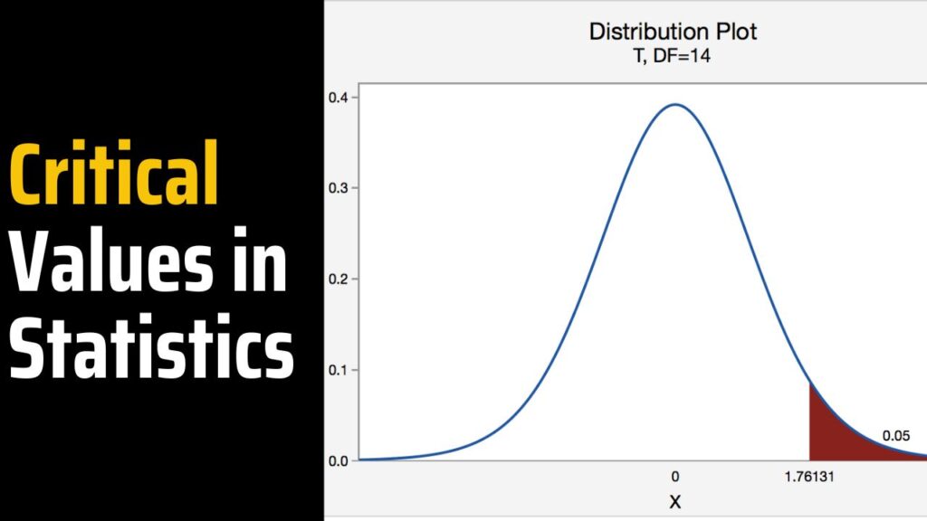
The concept of critical value is frequently used in statistics. Making judgments regarding testing hypotheses, calculating confidence intervals for a population-based sample of data, and other statistical issues can be assisted by understanding the critical values.

The critical value acts as a reference point for data analysis in addition to hypothesis testing. It supports statisticians in generating reliable inferences from data and maintaining the validity of their findings.

In this article, we will explore the critical value with its definition, confidence interval, types, and applications.

• Table of Contents

Critical Values

The critical value in statistics is a starting point used when comparing to a test statistic in hypothesis testing. It helps in deciding whether to reject or accept the null hypothesis. The null hypothesis typically posits that there is no significant difference or suggestion between variables under study.

In contrast, the alternative hypothesis suggests the opposite, stating that there is a significant difference or relationship. The critical value, which may or may not be an integer, is determined based on the desired significance level of the test and the distribution of the test statistic.

The test statistic that defines the upper and lower bounds of a confidence interval or the threshold of statistical significance in a test is known as the critical value. It indicates how far that you must go from the distribution’s mean in order to cover a specific amount of the overall variation in the data (i.e., 90%, 95%, 99%).

Your critical value will be the same in all scenarios if you are building a 95% confidence interval and utilizing a p = 0.05 statistical significance threshold.

Confidence interval

It is possible to evaluate the beginning of confidence for a one-tailed or two-tailed test. Study that the condition for a hypothesis test demands a 95% confidence interval. This is how the critical significance can be found.

Step 1: The confidence level is subtracted from 100 percent. 100% – 95% = 5%.

Step 2: You must transform this quantity to decimals. Thus, α = 5%.

Step 3: If the evaluation is one-tailed, phase 2’s alpha level will be the identical amount. However, the alpha level will be reduced by 2 if the test has two possible outcomes.

Step 4: The critical value can be found from the associated distribution table using the alpha value, based on the kind of test that was performed.

Types of Critical Values

F-critical value.

The study of variance & regression modeling depends heavily on the F-critical value. Such a value of significance determines whether to accept or reject the null hypothesis in a variance-based hypothesis test.

It is typically written as Fα, df1, df2, and where denotes the degree of significance and df1, and df2 denote the denominator’s and nominator’s respective degrees of freedom.

T-Critical Value

In testing for hypotheses for tiny samples where the population standard deviation is unidentified, the T-critical value is used. It aids in determining whether there is a notable difference between the sample mean and the population mean.

Z-Critical Value

When the sample size is significant and the data is distributed normally, the Z-critical value is used. For quantities and means, it is frequently utilized.

Chi-Square Critical Value

Both freedom testing & the fit quality analyses use the Chi-square critical value. It evaluates how category variables are related.

In this section, we will explore the critical value with the help of examples.

Calculate the critical value Z Left tail test if 𝛼 = 0.012.

Step 1: Find a confidence level

Subtract 𝛼 form 0.5, thus

Level of confidence = 0.5 – 0.012

Level of confidence = 0.488

Step 2: Using the Z table Find the table value

Step 3: Conclusion

Because the test is left tail the critical value becomes -2.26

With the sample size of 25 at a level of significance alpha = 0.025

level of significance

Degree of freedom

Df = k – 1, Df = 25 – 1

Then, we use one tail T distribution table at k = 24 and α = 0.025 is 2.0639

C = Critical value = 2.0639.

You can also utilize online tools to find critical values of t, z, f, and chi-square tests according to the distribution tables.

Daily life application

Drug effectiveness.

Let’s say a pharmaceutical business produces a brand-new medication with the promise of significantly lowering cholesterol. A sample of patients is chosen, and their blood cholesterol levels have been evaluated before and after taking the medication to test this.

It is possible to tell how a medicine has an effect that is statistically significant by contrasting the population’s mean to the critical value.

Election Polling

The possibility of error is affected by critical values. Voters’ opinions get recorded after selecting an appropriate collection of them. Analysts can determine the range in which genuine votes stand by computing the confidence interval using the critical value.

Final Words

In this article, we will explore the critical value with definitions, formulas, confidence intervals, types, and applications in detail. In addition, you can easily understand the critical value and related problems.

1: What is intended by critical value?

The dimension of the test statistic that specifies the upper and lower bounds of a confidence interval or that creates the level of statistical implication in a statistical test is denoted as the vital rate.

2: How do critical value and p-value differ from one another?

Therefore, the crucial interval identifies the range across which our test statistic must fall to qualify for H 0 to be accepted. The p-value is somewhat the reverse in that it emphasizes the region outside of the crucial period. Suppose H 0 is correct, it predicts the likelihood that t or more severe values would develop.

3: What are the two critical values?

It is -1.645 for a lower-tailed test. However, if a two-tailed test is used, the critical values for the estimated degrees of freedom and the column that matches are -1.96 and 1.96, respectively.

Other articles

Please read through some of our other articles with examples and explanations if you’d like to learn more.

• PLS-SEM model
• Principal Components Analysis
• Multivariate Analysis
• Friedman Test
• Chi-Square Test (Χ²)
• Effect Size
• Critical Values in Statistics
• Statistical Analysis
• Calculate the Sample Size for Randomized Controlled Trials
• Covariate in Statistics
• Avoid Common Mistakes in Statistics
• Standard Deviation
• Derivatives & Formulas
• Build a PLS-SEM model using AMOS
• Principal Components Analysis using SPSS
• Statistical Tools
• Type I vs Type II error
• Descriptive and Inferential Statistics
• Microsoft Excel and SPSS
• One-tailed and Two-tailed Test
• Parametric and Non-Parametric Test

Citation Styles

• APA Reference Page
• MLA Citations
• Chicago Style Format
• “et al.” in APA, MLA, and Chicago Style
• Do All References in a Reference List Need to Be Cited in Text?

Comparision

• Independent vs. Dependent Variable – MIM Learnovate
• Research Article and Research Paper
• Proposition and Hypothesis
• Principal Component Analysis and Partial Least Squares
• Academic Research vs Industry Research
• Clinical Research vs Lab Research
• Research Lab and Hospital Lab
• Thesis Statement and Research Question
• Quantitative Researchers vs. Quantitative Traders
• Premise, Hypothesis and Supposition
• Survey Vs Experiment
• Hypothesis and Theory
• Independent vs. Dependent Variable
• APA vs. MLA
• Ghost Authorship vs. Gift Authorship
• Basic and Applied Research
• Cross-Sectional vs Longitudinal Studies
• Survey vs Questionnaire
• Open Ended vs Closed Ended Questions
• Experimental and Non-Experimental Research
• Inductive vs Deductive Approach
• Null and Alternative Hypothesis
• Reliability vs Validity
• Population vs Sample
• Conceptual Framework and Theoretical Framework
• Bibliography and Reference
• Stratified vs Cluster Sampling
• Sampling Error vs Sampling Bias
• Internal Validity vs External Validity
• Full-Scale, Laboratory-Scale and Pilot-Scale Studies
• Plagiarism and Paraphrasing
• Research Methodology Vs. Research Method
• Mediator and Moderator
•   Dissertation Topic
• Thesis Statement
• Research Proposal
• Research Questions
• Research Problem
• Research Gap
• Types of Research Gaps
• Operationalization of Variables
• Literature Review
• Research Hypothesis
• Questionnaire
• Reliability
• Measurement of Scale
• Sampling Techniques
• Acknowledgements
• Research Methods
• Quantitative Research
• Qualitative Research
• Case Study Research
• Survey Research
• Conclusive Research
• Descriptive Research
• Cross-Sectional Research
• Theoretical Framework
• Conceptual Framework
• Triangulation
• Grounded Theory
• Quasi-Experimental Design
• Mixed Method
• Correlational Research
• Randomized Controlled Trial
• Stratified Sampling
• Ethnography
• Ghost Authorship
• Secondary Data Collection
• Primary Data Collection
• Ex-Post-Facto

Related Posts

11 examples of directional hypothesis, effect size (examples) and why does it matter, statistical analysis | 5 steps & examples, how to calculate the sample size for randomized controlled trials (rct), covariate in statistics: examples, what is primary data collection types, advantages, and disadvantages, understanding standard deviation: a deep dive into the key concepts, how do you avoid common mistakes in statistics, a glance at derivatives & formulas, how to build a pls-sem model using amos.

Comments are closed.

• school Campus Bookshelves
• menu_book Bookshelves
• perm_media Learning Objects
• login Login
• how_to_reg Request Instructor Account
• hub Instructor Commons
• Download Page (PDF)
• Download Full Book (PDF)
• Periodic Table
• Physics Constants
• Scientific Calculator
• Reference & Cite
• Tools expand_more
• Readability

selected template will load here

This action is not available.

8.1: The Elements of Hypothesis Testing

• Last updated
• Save as PDF
• Page ID 519

Learning Objectives

• To understand the logical framework of tests of hypotheses.
• To learn basic terminology connected with hypothesis testing.
• To learn fundamental facts about hypothesis testing.

Types of Hypotheses

A hypothesis about the value of a population parameter is an assertion about its value. As in the introductory example we will be concerned with testing the truth of two competing hypotheses, only one of which can be true.

Definition: null hypothesis and alternative hypothesis

• The null hypothesis , denoted \(H_0\), is the statement about the population parameter that is assumed to be true unless there is convincing evidence to the contrary.
• The alternative hypothesis , denoted \(H_a\), is a statement about the population parameter that is contradictory to the null hypothesis, and is accepted as true only if there is convincing evidence in favor of it.

Definition: statistical procedure

Hypothesis testing is a statistical procedure in which a choice is made between a null hypothesis and an alternative hypothesis based on information in a sample.

The end result of a hypotheses testing procedure is a choice of one of the following two possible conclusions:

• Reject \(H_0\) (and therefore accept \(H_a\)), or
• Fail to reject \(H_0\) (and therefore fail to accept \(H_a\)).

The null hypothesis typically represents the status quo, or what has historically been true. In the example of the respirators, we would believe the claim of the manufacturer unless there is reason not to do so, so the null hypotheses is \(H_0:\mu =75\). The alternative hypothesis in the example is the contradictory statement \(H_a:\mu <75\). The null hypothesis will always be an assertion containing an equals sign, but depending on the situation the alternative hypothesis can have any one of three forms: with the symbol \(<\), as in the example just discussed, with the symbol \(>\), or with the symbol \(\neq\). The following two examples illustrate the latter two cases.

Example \(\PageIndex{1}\)

A publisher of college textbooks claims that the average price of all hardbound college textbooks is \(\$127.50\). A student group believes that the actual mean is higher and wishes to test their belief. State the relevant null and alternative hypotheses.

The default option is to accept the publisher’s claim unless there is compelling evidence to the contrary. Thus the null hypothesis is \(H_0:\mu =127.50\). Since the student group thinks that the average textbook price is greater than the publisher’s figure, the alternative hypothesis in this situation is \(H_a:\mu >127.50\).

Example \(\PageIndex{2}\)

The recipe for a bakery item is designed to result in a product that contains \(8\) grams of fat per serving. The quality control department samples the product periodically to insure that the production process is working as designed. State the relevant null and alternative hypotheses.

The default option is to assume that the product contains the amount of fat it was formulated to contain unless there is compelling evidence to the contrary. Thus the null hypothesis is \(H_0:\mu =8.0\). Since to contain either more fat than desired or to contain less fat than desired are both an indication of a faulty production process, the alternative hypothesis in this situation is that the mean is different from \(8.0\), so \(H_a:\mu \neq 8.0\).

In Example \(\PageIndex{1}\), the textbook example, it might seem more natural that the publisher’s claim be that the average price is at most \(\$127.50\), not exactly \(\$127.50\). If the claim were made this way, then the null hypothesis would be \(H_0:\mu \leq 127.50\), and the value \(\$127.50\) given in the example would be the one that is least favorable to the publisher’s claim, the null hypothesis. It is always true that if the null hypothesis is retained for its least favorable value, then it is retained for every other value.

Thus in order to make the null and alternative hypotheses easy for the student to distinguish, in every example and problem in this text we will always present one of the two competing claims about the value of a parameter with an equality. The claim expressed with an equality is the null hypothesis. This is the same as always stating the null hypothesis in the least favorable light. So in the introductory example about the respirators, we stated the manufacturer’s claim as “the average is \(75\) minutes” instead of the perhaps more natural “the average is at least \(75\) minutes,” essentially reducing the presentation of the null hypothesis to its worst case.

The first step in hypothesis testing is to identify the null and alternative hypotheses.

The Logic of Hypothesis Testing

Although we will study hypothesis testing in situations other than for a single population mean (for example, for a population proportion instead of a mean or in comparing the means of two different populations), in this section the discussion will always be given in terms of a single population mean \(\mu\).

The null hypothesis always has the form \(H_0:\mu =\mu _0\) for a specific number \(\mu _0\) (in the respirator example \(\mu _0=75\), in the textbook example \(\mu _0=127.50\), and in the baked goods example \(\mu _0=8.0\)). Since the null hypothesis is accepted unless there is strong evidence to the contrary, the test procedure is based on the initial assumption that \(H_0\) is true. This point is so important that we will repeat it in a display:

The test procedure is based on the initial assumption that \(H_0\) is true.

The criterion for judging between \(H_0\) and \(H_a\) based on the sample data is: if the value of \(\overline{X}\) would be highly unlikely to occur if \(H_0\) were true, but favors the truth of \(H_a\), then we reject \(H_0\) in favor of \(H_a\). Otherwise we do not reject \(H_0\).

Supposing for now that \(\overline{X}\) follows a normal distribution, when the null hypothesis is true the density function for the sample mean \(\overline{X}\) must be as in Figure \(\PageIndex{1}\): a bell curve centered at \(\mu _0\). Thus if \(H_0\) is true then \(\overline{X}\) is likely to take a value near \(\mu _0\) and is unlikely to take values far away. Our decision procedure therefore reduces simply to:

• if \(H_a\) has the form \(H_a:\mu <\mu _0\) then reject \(H_0\) if \(\bar{x}\) is far to the left of \(\mu _0\);
• if \(H_a\) has the form \(H_a:\mu >\mu _0\) then reject \(H_0\) if \(\bar{x}\) is far to the right of \(\mu _0\);
• if \(H_a\) has the form \(H_a:\mu \neq \mu _0\) then reject \(H_0\) if \(\bar{x}\) is far away from \(\mu _0\) in either direction.

Think of the respirator example, for which the null hypothesis is \(H_0:\mu =75\), the claim that the average time air is delivered for all respirators is \(75\) minutes. If the sample mean is \(75\) or greater then we certainly would not reject \(H_0\) (since there is no issue with an emergency respirator delivering air even longer than claimed).

If the sample mean is slightly less than \(75\) then we would logically attribute the difference to sampling error and also not reject \(H_0\) either.

Values of the sample mean that are smaller and smaller are less and less likely to come from a population for which the population mean is \(75\). Thus if the sample mean is far less than \(75\), say around \(60\) minutes or less, then we would certainly reject \(H_0\), because we know that it is highly unlikely that the average of a sample would be so low if the population mean were \(75\). This is the rare event criterion for rejection: what we actually observed \((\overline{X}<60)\) would be so rare an event if \(\mu =75\) were true that we regard it as much more likely that the alternative hypothesis \(\mu <75\) holds.

In summary, to decide between \(H_0\) and \(H_a\) in this example we would select a “rejection region” of values sufficiently far to the left of \(75\), based on the rare event criterion, and reject \(H_0\) if the sample mean \(\overline{X}\) lies in the rejection region, but not reject \(H_0\) if it does not.

The Rejection Region

Each different form of the alternative hypothesis Ha has its own kind of rejection region:

• if (as in the respirator example) \(H_a\) has the form \(H_a:\mu <\mu _0\), we reject \(H_0\) if \(\bar{x}\) is far to the left of \(\mu _0\), that is, to the left of some number \(C\), so the rejection region has the form of an interval \((-\infty ,C]\);
• if (as in the textbook example) \(H_a\) has the form \(H_a:\mu >\mu _0\), we reject \(H_0\) if \(\bar{x}\) is far to the right of \(\mu _0\), that is, to the right of some number \(C\), so the rejection region has the form of an interval \([C,\infty )\);
• if (as in the baked good example) \(H_a\) has the form \(H_a:\mu \neq \mu _0\), we reject \(H_0\) if \(\bar{x}\) is far away from \(\mu _0\) in either direction, that is, either to the left of some number \(C\) or to the right of some other number \(C′\), so the rejection region has the form of the union of two intervals \((-\infty ,C]\cup [C',\infty )\).

The key issue in our line of reasoning is the question of how to determine the number \(C\) or numbers \(C\) and \(C′\), called the critical value or critical values of the statistic, that determine the rejection region.

Definition: critical values

The critical value or critical values of a test of hypotheses are the number or numbers that determine the rejection region.

Suppose the rejection region is a single interval, so we need to select a single number \(C\). Here is the procedure for doing so. We select a small probability, denoted \(\alpha\), say \(1\%\), which we take as our definition of “rare event:” an event is “rare” if its probability of occurrence is less than \(\alpha\). (In all the examples and problems in this text the value of \(\alpha\) will be given already.) The probability that \(\overline{X}\) takes a value in an interval is the area under its density curve and above that interval, so as shown in Figure \(\PageIndex{2}\) (drawn under the assumption that \(H_0\) is true, so that the curve centers at \(\mu _0\)) the critical value \(C\) is the value of \(\overline{X}\) that cuts off a tail area \(\alpha\) in the probability density curve of \(\overline{X}\). When the rejection region is in two pieces, that is, composed of two intervals, the total area above both of them must be \(\alpha\), so the area above each one is \(\alpha /2\), as also shown in Figure \(\PageIndex{2}\).

The number \(\alpha\) is the total area of a tail or a pair of tails.

Example \(\PageIndex{3}\)

In the context of Example \(\PageIndex{2}\), suppose that it is known that the population is normally distributed with standard deviation \(\alpha =0.15\) gram, and suppose that the test of hypotheses \(H_0:\mu =8.0\) versus \(H_a:\mu \neq 8.0\) will be performed with a sample of size \(5\). Construct the rejection region for the test for the choice \(\alpha =0.10\). Explain the decision procedure and interpret it.

If \(H_0\) is true then the sample mean \(\overline{X}\) is normally distributed with mean and standard deviation

\[\begin{align} \mu _{\overline{X}} &=\mu \nonumber \\[5pt] &=8.0 \nonumber \end{align} \nonumber \]

\[\begin{align} \sigma _{\overline{X}}&=\dfrac{\sigma}{\sqrt{n}} \nonumber \\[5pt] &= \dfrac{0.15}{\sqrt{5}} \nonumber\\[5pt] &=0.067 \nonumber \end{align} \nonumber \]

Since \(H_a\) contains the \(\neq\) symbol the rejection region will be in two pieces, each one corresponding to a tail of area \(\alpha /2=0.10/2=0.05\). From Figure 7.1.6, \(z_{0.05}=1.645\), so \(C\) and \(C′\) are \(1.645\) standard deviations of \(\overline{X}\) to the right and left of its mean \(8.0\):

\[C=8.0-(1.645)(0.067) = 7.89 \; \; \text{and}\; \; C'=8.0 + (1.645)(0.067) = 8.11 \nonumber \]

The result is shown in Figure \(\PageIndex{3}\). α = 0.1

The decision procedure is: take a sample of size \(5\) and compute the sample mean \(\bar{x}\). If \(\bar{x}\) is either \(7.89\) grams or less or \(8.11\) grams or more then reject the hypothesis that the average amount of fat in all servings of the product is \(8.0\) grams in favor of the alternative that it is different from \(8.0\) grams. Otherwise do not reject the hypothesis that the average amount is \(8.0\) grams.

The reasoning is that if the true average amount of fat per serving were \(8.0\) grams then there would be less than a \(10\%\) chance that a sample of size \(5\) would produce a mean of either \(7.89\) grams or less or \(8.11\) grams or more. Hence if that happened it would be more likely that the value \(8.0\) is incorrect (always assuming that the population standard deviation is \(0.15\) gram).

Because the rejection regions are computed based on areas in tails of distributions, as shown in Figure \(\PageIndex{2}\), hypothesis tests are classified according to the form of the alternative hypothesis in the following way.

Definitions: Test classifications

• If \(H_a\) has the form \(\mu \neq \mu _0\) the test is called a two-tailed test .
• If \(H_a\) has the form \(\mu < \mu _0\) the test is called a left-tailed test .
• If \(H_a\) has the form \(\mu > \mu _0\)the test is called a right-tailed test .

Each of the last two forms is also called a one-tailed test .

Two Types of Errors

The format of the testing procedure in general terms is to take a sample and use the information it contains to come to a decision about the two hypotheses. As stated before our decision will always be either

• reject the null hypothesis \(H_0\) in favor of the alternative \(H_a\) presented, or
• do not reject the null hypothesis \(H_0\) in favor of the alternative \(H_0\) presented.

There are four possible outcomes of hypothesis testing procedure, as shown in the following table:

As the table shows, there are two ways to be right and two ways to be wrong. Typically to reject \(H_0\) when it is actually true is a more serious error than to fail to reject it when it is false, so the former error is labeled “ Type I ” and the latter error “ Type II ”.

Definition: Type I and Type II errors

In a test of hypotheses:

• A Type I error is the decision to reject \(H_0\) when it is in fact true.
• A Type II error is the decision not to reject \(H_0\) when it is in fact not true.

Unless we perform a census we do not have certain knowledge, so we do not know whether our decision matches the true state of nature or if we have made an error. We reject \(H_0\) if what we observe would be a “rare” event if \(H_0\) were true. But rare events are not impossible: they occur with probability \(\alpha\). Thus when \(H_0\) is true, a rare event will be observed in the proportion \(\alpha\) of repeated similar tests, and \(H_0\) will be erroneously rejected in those tests. Thus \(\alpha\) is the probability that in following the testing procedure to decide between \(H_0\) and \(H_a\) we will make a Type I error.

Definition: level of significance

The number \(\alpha\) that is used to determine the rejection region is called the level of significance of the test. It is the probability that the test procedure will result in a Type I error .

The probability of making a Type II error is too complicated to discuss in a beginning text, so we will say no more about it than this: for a fixed sample size, choosing \(alpha\) smaller in order to reduce the chance of making a Type I error has the effect of increasing the chance of making a Type II error . The only way to simultaneously reduce the chances of making either kind of error is to increase the sample size.

Standardizing the Test Statistic

Hypotheses testing will be considered in a number of contexts, and great unification as well as simplification results when the relevant sample statistic is standardized by subtracting its mean from it and then dividing by its standard deviation. The resulting statistic is called a standardized test statistic . In every situation treated in this and the following two chapters the standardized test statistic will have either the standard normal distribution or Student’s \(t\)-distribution.

Definition: hypothesis test

A standardized test statistic for a hypothesis test is the statistic that is formed by subtracting from the statistic of interest its mean and dividing by its standard deviation.

For example, reviewing Example \(\PageIndex{3}\), if instead of working with the sample mean \(\overline{X}\) we instead work with the test statistic

\[\frac{\overline{X}-8.0}{0.067} \nonumber \]

then the distribution involved is standard normal and the critical values are just \(\pm z_{0.05}\). The extra work that was done to find that \(C=7.89\) and \(C′=8.11\) is eliminated. In every hypothesis test in this book the standardized test statistic will be governed by either the standard normal distribution or Student’s \(t\)-distribution. Information about rejection regions is summarized in the following tables:

Every instance of hypothesis testing discussed in this and the following two chapters will have a rejection region like one of the six forms tabulated in the tables above.

No matter what the context a test of hypotheses can always be performed by applying the following systematic procedure, which will be illustrated in the examples in the succeeding sections.

Systematic Hypothesis Testing Procedure: Critical Value Approach

• Identify the null and alternative hypotheses.
• Identify the relevant test statistic and its distribution.
• Compute from the data the value of the test statistic.
• Construct the rejection region.
• Compare the value computed in Step 3 to the rejection region constructed in Step 4 and make a decision. Formulate the decision in the context of the problem, if applicable.

The procedure that we have outlined in this section is called the “Critical Value Approach” to hypothesis testing to distinguish it from an alternative but equivalent approach that will be introduced at the end of Section 8.3.

Key Takeaway

• A test of hypotheses is a statistical process for deciding between two competing assertions about a population parameter.
• The testing procedure is formalized in a five-step procedure.

T Critical Value: Definition, Formula, Interpretation, and Examples

5 months ago

When delving into the world of hypothesis testing in statistics, one term that you will frequently encounter is the " t critical value ." But what exactly does it mean, and why is it so important in the realm of statistical analysis? 

This article will break down the concept of the t critical value , explaining its definition, how to calculate it, and how to interpret its results with easy-to-understand examples.

What is t-critical value?

The t critical value is a key component in the world of hypothesis testing, which is a method statisticians use to test the validity of a claim or hypothesis. 

In simpler terms, when researchers want to understand if the difference between two groups is significant or just happened by chance, they use a t-test and, by extension, the t critical value .

Why is it called “t-critical value”?

The " t " in the t critical value comes from the t-distribution , which is a type of probability distribution. A probability distribution is essentially a graph that shows all possible outcomes of a particular situation and how likely each outcome is. 

The t-distribution is used when the sample size is small, and the population variance ( i.e., how spread out the data is ) is unknown.

The Formula for Calculating the T Critical Value:

The formula for calculating the t critical value is as follows:

\[t = \frac{(\bar{X}_1 - \bar{X}_2)}{(s_p \sqrt{\frac{2}{n}})}\]

• t = t critical value
• x̄ 1 and x̄ 2 = means (i.e., averages) of the two groups being compared.
• s = standard deviation of the sample (i.e., a measure of how spread out the data is). 
• n = sample size (i.e., the number of data points).

This formula helps to calculate the difference between the average values of the two groups, taking into account the variability of the data and the sample size.

Interpreting the T Critical Value:

Once the t critical value has been calculated, it can be compared to the t distribution to determine the significance of the results. 

• If the calculated t value falls within the critical region of the t distribution , we can reject the null hypothesis and conclude that there is a significant difference between the two groups. 
• If the t value falls outside the critical region, we fail to reject the null hypothesis , suggesting that there is not a significant difference between the two groups.

Imagine a teacher who wants to know if a new teaching method is more effective than the traditional method. They divide their students into two groups: one group is taught using the new method, and the other group is taught using the traditional method. After a test, they calculate the average scores of the two groups and use the t-test formula to find the t critical value .

If the t critical value is greater than the critical value from the t-distribution, the teacher can conclude that the new teaching method is significantly more effective than the traditional method.

How to calculate the t-critical value?

To calculate the t critical value , you will need the following information:

The level of significance (α): This is the probability of rejecting the null hypothesis when it is true. Common levels of significance are 0.05 , 0.01 , and 0.10 .

The degrees of freedom (df): This value depends on the sample size and the type of t-test you are conducting. For a one-sample t-test, the degrees of freedom is equal to the sample size minus one (n - 1) . For a two-sample t-test , the degrees of freedom can be calculated using the formula:

\[df = \frac{\left(\frac{s_1^2}{n_1} + \frac{s_2^2}{n_2}\right)^2}{\frac{\left(\frac{s_1^2}{n_1}\right)^2}{n_1 - 1} + \frac{\left(\frac{s_2^2}{n_2}\right)^2}{n_2 - 1}}\]

• s 1 and s 2 are the standard deviations of the two samples
• n 1 and n 2  are the sample sizes.

The type of t-test: There are different types of t-tests , including one-sample, two-sample, and paired-sample t-tests . The type of t-test you are conducting will affect the degrees of freedom and the critical value.

Once you have this information, you can use a t-distribution table or statistical software to find the t-critical value . 

Note: A table is provided at the end of the article.

Solved problem:

Suppose you are conducting a study to compare the test scores of two different teaching methods. The collected data from two independent samples is:

• Sample 1 (Teaching Method A): n 1 = 25 students, mean test score x̄ 1 = 78, and standard deviation s 1 = 10.
• Sample 2 (Teaching Method B): n 2 = 3 0 students, mean test score x̄ 2 = 82 , and standard deviation s 2 = 12 .

You want to test the null hypothesis that there is no significant difference between the two teaching methods at a 0.05 level of significance.

Steps to Calculate the t Critical Value:

Step 1: Calculate the pooled standard deviation ( s p ).

\[s_p = \sqrt{\frac{{(n_1 - 1) s_1^2 + (n_2 - 1) s_2^2}}{{n_1 + n_2 - 2}}}\]

Substituting the values, we get:

\[s_p = \sqrt{\frac{{(25 - 1) 10^2 + (30 - 1) 12^2}}{{25 + 30 - 2}}}\]

\[s_p \approx 11.1\]

Step 2: Calculate the t-statistic:

\[t = \frac{{50 - 52}}{{11.1 \sqrt{\frac{2}{25}}}}\]

\[t \approx -0.4\]

Step 3: Determine the degrees of freedom (df) for a two-sample t-test:

Substitute the values:

\[df = \frac{\left(\frac{10^2}{25} + \frac{12^2}{30}\right)^2}{\frac{\left(\frac{10^2}{25}\right)^2}{25 - 1} + \frac{\left(\frac{12^2}{30}\right)^2}{30 - 1}}\]

\[df \approx 53\]

Step 4: Determine the critical t-value from the t-value table .

For a significance level of 0.05 (two-tailed test), and degrees of freedom (df) closest to 53 , you would look up the value in the table. In this case, let's say the critical value for 50 degrees of freedom at the 0.05 significance level is 2.009.

Step 5: Compare the calculated t-statistic to the critical t-value.

In this example, the calculated t-statistic ( -0.4 ) is less than the critical t-value ( 2.009 ), therefore we would fail to reject the null hypothesis. This means that there is no significant difference between the two sample means.

T-value table:

In this table, the leftmost column lists the degrees of freedom ( df ), and the top row lists the significance levels ( 0.10, 0.05, 0.025, 0.01, and 0.005 ). Each cell in the table contains the critical t-value for the corresponding degrees of freedom and significance level. 

Here is how you can find the t critical value using this t-distribution table:

• Find the row that corresponds to your degrees of freedom .
• Find the column that corresponds to your level of significance .
• The value where the row and column intersect is the t critical value .

For example, if you have 7 degrees of freedom and are conducting a test at the 0.05 significance level , the critical t-value is 1.895.

Conclusion:

By understanding the definition, formula, and interpretation of the t critical value, you will be better equipped to evaluate research studies and make informed decisions based on data. So, the next time you come across a study that uses a t-test, you'll know exactly what's going on!

Recent Blogs

F Critical Value: Definition, formula, and Calculations

Understanding z-score and z-critical value in statistics: A comprehensive guide

P-value: Definition, formula, interpretation, and use with examples

Criticalvaluecalculator.com is a free online service for students, researchers, and statisticians to find the critical values of t and z for right-tailed, left tailed, and two-tailed probability.

Information

• Privacy Policy
• Terms of Services

What is Critical Value? Defined & Explained with Examples

In the field of statistics, the concept of critical value keeps an exceptional position. It plays a key role in several analytical and scientific fields confidence intervals, hypothesis testing as well as in decision-making. The critical value is integral and helps in dealing with data analysis.

Definition of Critical Value:

Z-distribution (normal distribution):, t-distribution:, chi-square distribution:, f-distribution:, role of critical values:, importance of critical values:.

A test statistic is measured against a critical value while conducting a hypothesis test. We reject the null hypothesis if the test statistic is greater than the critical threshold. Critical value is a specific value that comes from a test statistic’s sample distribution, such as the t-distribution or the normal distribution, and it is employed to observe whether it is to accept or reject the null hypothesis (H 0 ).

In this article, we have elaborated on the important term critical value. We will present its definition, formula, and importance. We will also give some examples to grasp the concept of the critical value.

In statistical hypothesis testing, the critical value is a threshold or boundary that assists in determining whether to accept or reject the null hypothesis. In a statistical test, the value distinguishes between the zone of acceptance and the region of rejection.

The desired significance level (α), which denotes the likelihood of making a Type I mistake (wrongly rejecting a valid null hypothesis), is what determines it. The significance level commonly indicated as (alpha), which represents the likelihood of committing a Type I mistake (erroneously rejecting a valid null hypothesis), is used to calculate critical values.

Formula for Critical Value:

The formula for calculating critical values depends on the statistical distribution and the desired significance level (α). Here are a few common distributions and their associated critical value formulas

For a standard normal distribution, you can find critical values using the z-table or a calculator. The critical value is denoted as zα/2, where α/2 is half of the significance level. For example, if α = 0.05 (a common choice), then the critical value would be z0.025.

When working with small sample sizes or when the population standard deviation is unknown, the t-distribution is used. The significance level and degrees of freedom (df) are used to calculate the critical value. Utilizing statistical tables or software, you could find the t-critical values.

The number of degrees of freedom and the level of significance are what decide the chi-square test’s extremely important value. The formula is written asχ²α that stands for the significance level.

Critical values are determined using the F-distribution and are dependent on the degrees of freedom for the numerator and denominator as well as the significance level for ANOVA and other F-tests.

Critical values serve as decision points in hypothesis testing. When conducting a hypothesis test, you compare the test statistic (calculated from your sample data) to the critical value.

The critical value helps determine whether to reject the null hypothesis or fail to reject it. If the test statistic falls in the rejection region (beyond the critical value), you reject the null hypothesis; otherwise, you do not reject it.

Statistical Significance: Critical values help establish statistical significance. They provide a clear threshold for determining whether the observed data is unlikely to occur by chance alone.

• Objective Decision-Making: Critical values offer an objective basis for making decisions in hypothesis testing. They help prevent subjective judgments and biases.
• Standardization: Critical values provide a standardized approach to hypothesis testing, making it possible for researchers and statisticians worldwide to use the same principles and criteria.
• Quality Control: In fields such as manufacturing and quality control, critical values are used to set tolerance limits, ensuring products meet certain standards.
• Scientific Research: Critical values play a crucial role in scientific research, allowing researchers to draw conclusions and make inferences based on data.

Consider that a one-tailed t-test is conducted on data having:

Sample size = 15

α = 0.025, Find the critical value.

Step 1: Given data

Degree of freedom (df) = n – 1

df = 15 – 1

Step 2: Using t-distribution table,

T(0.025, 140) = 2.145

Therefore, the critical value for the given one-tailed t-distribution is 2.145

A t table calculator is an online resource to find the t critical value of the given values according to the distribution table in couple of seconds.

Determine the critical value for a two-tailed f-test conducted on the following samples at a significance level (α) of 95%.

Variance = 120, sample size = 25

Variance = 80, sample size = 17

n 1 = 25, n 2 = 17

α = 0.05 (95% confidence level)

df 1 = n 1 – 1

df 1 = 25 – 1

df 2 = n 2 – 2

df 2 = 17 – 1

Step 3: We will observe the f distribution table for α = 0.05.

The value at the intersection of the 24 th column and the 16 th row.

F(24, 16) = 2.24

Critical value = 2.24

We can summarize the whole article as the critical values are essential for statistical analysis and offer a distinct framework for evaluating hypotheses and making decisions. In this article, we have addressed an important term critical value, its definition, and its importance.

Related Posts:

• Variance and Standard Deviation: A Complete Guide with Examples

Leave a Comment Cancel reply

Save my name, email, and website in this browser for the next time I comment.

• school Campus Bookshelves
• menu_book Bookshelves
• perm_media Learning Objects
• login Login
• how_to_reg Request Instructor Account
• hub Instructor Commons
• Download Page (PDF)
• Download Full Book (PDF)
• Periodic Table
• Physics Constants
• Scientific Calculator
• Reference & Cite
• Tools expand_more
• Readability

selected template will load here

This action is not available.

7.5: Critical values, p-values, and significance level

• Last updated
• Save as PDF
• Page ID 195834

• Stock Compare
• Nifty Heatmap
• Superstar Portfolio
• Corporate Actions
• *Now Available in Hindi

Introduction to Critical Values in Statistics: Concepts and Examples

by Trade Brains | Jan 18, 2023 | 4:23 pm | Articles | 0 comments

In statistical hypothesis testing, a critical value is a point on the test distribution that is used to determine the rejection region, also known as the acceptance region. The critical value separates the area where the null hypothesis is rejected from the area where it is not rejected. 

In this article, we will explore the definition, and concept of critical values in more detail, including how they are calculated, and provide practical examples of their use in different statistical tests.

Definition of critical value: 

Critical value can be defined as a value that is compared to a test statistic in hypothesis testing to determine whether the null hypothesis is to be rejected or not.

The concept of critical values:

A critical value is a fixed point on the test distribution, typically represented by a z-score or t-score, that separates the acceptance region from the rejection region. The acceptance region is the area of the test distribution where the null hypothesis is not rejected. 

While the rejection region is the area where the null hypothesis is rejected. The critical value is chosen based on the desired level of significance, also known as the alpha level.

For example , if the desired level of significance is 0.05, this means that there is a 5% chance of making a type I error, or incorrectly rejecting the null hypothesis. The critical value for a 0.05 level of significance will be different for different types of test distributions, such as the normal distribution or the t-distribution.

Calculation of critical values:

The critical value is calculated based on the test distribution, the level of significance, and the type of test being performed. For example, in a two-tailed test, the critical value is calculated as the point that separates the outer 2.5% of the test distribution on either side. 

In a one-tailed test, the critical value is calculated as the point that separates the outer 5% of the test distribution on one side.

The critical value can be calculated using a critical value table, which lists the critical values for different levels of significance and test distributions. Alternatively, the critical value can be calculated using a calculator or a software program that performs statistical tests.

Practical examples of critical values:

A/B testing:  

A/B testing is a statistical method used to compare two versions of a product or website to determine which one performs better. In A/B testing, a critical value is used to determine the significance of the difference between the two versions. 

For example , if the critical value for a 0.05 level of significance is -1.96 for a two-tailed test, and the calculated z-score is -2.0, this means that the difference between the two versions is statistically significant.

T-test:  

A t-test is a statistical test used to determine if there is a significant difference between the means of two groups. In a t-test, a critical value is used to determine the significance of the difference between the means.

For example, if the critical value for a 0.05 level of significance is -1.645 for a two-tailed test, and the calculated t-score is -1.7, this means that the difference between the means is statistically significant.

Chi-square test:  

A chi-square test is a statistical test used to determine if there is a significant difference between the observed frequencies and the expected frequencies in a frequency distribution. In a chi-square test, a critical value is used to determine the significance of the difference between the observed and expected frequencies. 

For example , if the critical value for a 0.05 level of significance is 3.84 for a chi-square distribution with 3 degrees of freedom, and the calculated chi-square value is 4.0, this means that the difference between the observed and expected frequencies is statistical.  

You can try a criticalvaluecalculator.com for the calculations of t-value, f-value, R-value, z-value, and chi-square critical values according to critical value tables. 

Example section: 

In this section, we’ll describe some mathematical examples to understand the method of finding the critical value of different samples. 

Example 1: Calculate the z critical value if α = 0.3

Solution: 

Step 1: Division

Divide 0.3 by “2”.

= 0.3 / 2 

= 0.15 

Step 2: Subtraction

Subtract the value of α from 1. 

= 1 – 0.15 

Step 3: Check the table.  

Here’s the z-distribution table. 

The value matches at 1.0 + 0.04. 

So, the approximate value is 1.04 . 

Example 2: Calculate the t critical value if α = 0.02 and the degree of freedom is 45 

Step 1: If both α and degree of freedom are given then you just have to check the table to find out the value.  

On 45 degrees the value is 2.4121 for the two-tailed T-test. 

Summary: 

In this article, we have studied the basic definition of critical values, and we have learned a deep introduction to the basics of this topic. We have also discussed practical examples and methods to calculate the T-critical value and z-critical value. 

Further in this article, we have discussed all the types of critical values. You have witnessed that it is not a difficult topic, and now you can solve all the problems related to this topic. Happy testing!

No related posts.

Submit a Comment Cancel reply

Your email address will not be published. Required fields are marked *

Save my name, email, and website in this browser for the next time I comment.

Recent News

• Midcap stocks with a high Piotroski Score of up to 8; Do you hold any? 
• Stock in Focus: Pharma stock to buy now for an upside of up to 47%
• Smallcap stocks in which DIIs have increased their stake by up to 10.47% 
• Stock with market share of 43% in Pain management Products to keep an eye on
• ₹10,000 to ₹16.60 Lakhs; Multibagger stock delivers 16,500% returns in 4 years 
• Multibagger stock hit 5% upper circuit after delivering 6 Greenfield Air Separation to US client 
• FMCG stock jumps 6% after commissioning its new plant for Cocoa Butter and other products 
• High-Yield ETFs for Effective Income Investing