assignment on aerial photo

Introduction to Aerial Photography

Aerial photography is the science and technology of capturing photos of the land surface from any flying object such as airplane, helicopter, drone etc. Gaspar Felix Tournachon was first first person to capture an aerial photograph in 1858 from an air balloon. However, Talbert Abrams is known as the father of Aerial Photography. He was a pilot with the US Marine Corps and took widespread aerial photography. Afterwards, aerial photography became an important source of information. Therefore a researcher must understand the nature of aerial photography and their usage. In this article, we will provide a brief introduction to aerial photography and try to understand the definition of aerial photographs, its characteristics, advantages and uses.

Definition of Aerial Photograph

• Definition: An aerial photograph refers to a large scale photo captured from a camera attached to any flying machine. The flying machine may be helicopter, aeroplane, drone, etc.
• The large scale photographs show a small area on a piece of paper with great details .
• The scale of the photograph depends on the altitude of the aeroplane . On the one hand, if the aeroplane is taking the photo from higher altitude, the scale becomes smaller. On the contrary, if the aeroplane is taking the photo from lower altitude the scale becomes larger.
• Also read Types of Aerial Phtography .

Characteristics of Aerial Photographs

Aerial photographs have certain features which differentiate the from the other types of imageries and photos.

• Aerial photographs are a qualitative source of information.
• The aerial photos are generally large scale photos with a scale less than 1:30000 . Hence, we can see the objects on the ground in great detail. The general maps do not show such characteristics on the ground.
• The aerial photographs are taken by precision cameras , therefore, errors are minimized while capturing photos from a flying object.
• Aerial camera devices have very high sensitivity and capture a greater range of information than the human eye. Human eye can capture the light with a wavelength of 0.4 to 0.7 micrometers whereas the aerial camera can capture the wavelength of 0.3 to 0.9 micrometer . Hence, we receive a greater amount of information.
• The aerial photos show the objects in their true shape and size , hence, it is easier for the humans to analyze an area without the help of a computer.

Advantages of Aerial Photography

• Improved Vantage Point: Aerial photos provide us with a bird’s view perspective. We can see a large area and its features in relation to each other.
• Historical Record: These photos show the real-time situation of a place at a particular time. Therefore, they become a historical record and we can use them to study past characteristics of land-use.
• Greater Information: The aerial photos capture a greater range of electromagnetic spectrum. Therefore, aerial photos show even those features of earth which can not be seen by human eye.
• Three Dimensional Views: A single aerial photo shows any given feature from two different angles. Therefore, we can see that particular feature in three dimensions with the help of a  Pocket Stereoscope .

Uses of Aerial Photography

Like any other source of information, we use aerial photography for many purposes as follows.

• Reconnaissance Survey : These are also called preliminary surveys. These surveys are extensive study of an area before implementation of a project in that area. For example, before building an airport in an area, the planners will try to assess the availability of plain area, topographical barriers, presence of rivers etc. to see feasibility of an airport.
• Photogrammetry : It refers to the science and technology of making correct estimation of shape, size and altitude of objects on aerial photographs. Using photogrammetry, the cartographers use aerial photography for topographical mapping. The aerial photographs show topographical features in three dimensional view. We can compute the altitude of each and every object in aerial photography by using  Stereo Micrometer or stereoscopy . Ultimately, we can draw the contours based on measurements through stereo micrometer.
• Making Topographical Maps : The cartographers use the aerial photographs to draw   Topographic Maps . Topographical maps show the objects on the ground in representative colors e.g. water bodies in blue, forests in green etc. Topographical maps are of great importance for planning and implementation of policies.
• Interpretation of Aerial Photo : By interpretation of aerial photograph’s features, we can have a general understanding of the study area. For instance, if the farms in aerial photos look as white squares, it means the area is unirrigated. Similarly, by studying the shadow of objects, we can understand the topographic undulations in the area. The interpretation of aerial photographs provides important qualitative information about an area.
• Micro-level Planning : Since, the aerial photos are large scale images, the planners can plan at micro level. They may plan for very small objects such as trees, houses, ponds etc. before planning and executing a project.

In summary, we can conclude that aerial photography is a quick and effective visual tool to collect and analyze information. The aerial photographs are large scale, so it shows smaller objects in great detail. Further, it is a qualitative source of information and helps in efficient execution of projects of socio-economic welfare over the focus area. 

Kulwinder Singh is an alumni of Jawaharlal Nehru University, New Delhi and working as Assistant Professor of Geography at Pt. C.L.S. Government College, Kurukshetra University. He is a passionate teacher and avid learner.

Share this:

• Click to share on WhatsApp (Opens in new window)
• Click to share on Telegram (Opens in new window)
• Click to share on Facebook (Opens in new window)

Principles and Applications of Aerial Photography

Desk based research is not just about reading papers for vital pieces of information, it is not just about tables, graphs, facts and figures. For many, primary data is all around us; aerial photography, for example, is an important source of information for researchers in landscape studies. This includes disciplines such as Landscape Archaeology (the study of how humans used landscapes in the past), Human Geography (how modern humans utilise the landscape) and climate science (to determine land use and conditions; to track - for example - the growth and retreat of seasonal ice and water levels or invasive flora species).

What Is Aerial Photography and How Does It Work?

Aerial photography is - as it sounds - the process of taking photographs from the air, but there is more to it than simply using a light aircraft or helicopter and flying up to take photographs. There are many elements to an aerial survey that must be considered to ensure that the data is useful enough to extrapolate whatever is being investigated. It is often difficult to see elements of the landscape on the ground, features can easily be missed, and what might seem like an insignificant bump from ground level can become more significant in a wider context (2); some landscape types are difficult to access on foot so aerial photographs are vital to study and map them.

They have been used as a method of landscape studies for over a century (3) , especially in archaeology and researchers have learnt much about the world around us; its applications today are broad and coupled with the growing technology of GIS (geographic information systems), the potential means that the method will not become obsolete any time soon. Aerial photographs are taken in two basic forms and both have different uses and applications: oblique and vertical. Even today in an age of high quality digital imaging, black and white images are preferred - partly because they are cheaper but also partly because the contrast of black, white and greys makes it easier to pick out features (7) .

These images are usually taken at an angle, typically 45 degrees but as they are often taken manually, they can be whatever angle gives the best view of the feature or landscape. The oblique image is primarily used in archaeology to take a wider context of a feature and the area around it, and also to give depth. Nearly always taken at a much lower elevation than the vertical image and in few numbers, its application is fairly limited and often taken for a specific purpose (8) . There is a problem in perspective because the farther away a feature is, the smaller it will appear: nearer objects of comparable size appear larger than those that are farther away so it is often best to take a selection or to use a frame of reference on the ground for perspective purposes. These images are taken from small fixed-wing aircraft and helicopters (3) and are perfectly suited for monitoring erosion of features and monuments throughout the year and over the course of many decades (4).

Oblique Photographs: When Best to Take Them?

The time of year is vital and many see winter as the perfect season to take aerial photographs. There are many reasons for this, not least of all that it is easier to see features in fields that do not have crops and will not be ploughed for several more months. Surviving features beneath the surface will often show up darker due to the shallower levels of soil. Snowy and frosty conditions perfectly emphasise ridges and features and they can be photographed with a clarity not seen at any other time of the year. The low level to which the sun rises casts much longer shadows, making visibility of above ground features much easier to spot. The perfect example here is relict medieval ridge and furrow features (9) .

That's not to say that the warmer months and longer hours of light are not conducive to aerial photography. If there are stone remains beneath a surface, crops will grow shallower as they cannot put down as much root and features will show up as crop marks. Late evening conditions also cast longer shadows and the differing light levels between morning, afternoon and evening can add depth when comparing multiple images of the same feature(s) over the course of a day (9) .

Taking a photograph straight down over a landscape is the more familiar form of aerial photograph. It is a plan view so there is no perspective to distort the image. This also means that it is difficult to read the lay of the land such as changes in height - though there is a work around to create 3D image through stereoscopic views, using a device to examine two at once. This usually gives a good impression of the variation in the elevation of land (8) . They are taken at regular heights for consistency so it is easier to compare contexts of a landscape taken on the same day, or many years apart to examine development. Rarely used in archaeological applications except perhaps sometimes to find interesting earthworks and other sites that are easily missed on the ground (8) , they cover a much wider area (6) and focus on topography rather than specific details (4) .

Vertical Photographs: When Best to Take Them?

As a rule, vertical aerial photographs are easier to interpret than oblique photographs because of the standardised ways in which they are taken - with set scales and at a single non-arbitrary angle (10) . The same advantages generally apply to vertical as they do for oblique, but you will lack the perspective, the depth and the 3D effect even with the weather conditions mentioned above. At higher levels, you may miss crop and soil marks. If it is an overview you require, then vertical photography is the best way to go.

History of Aerial Photography and Survey

The first aerial photograph was oblique and taken of a French village in the late 19 th century. The man who took it - photographer Gaspar Felix Tournachon - patented the concept of using aerial photographs to compile maps (5) ; it was to prove much more effective than the time-consuming ground surveys that had then been the more commonly-used method of the national mapping organisations that developed throughout the 19 th century (such as the UK's Ordnance Survey). George R. Lawrence took aerial photographs of San Francisco in 1906 following the devastating earthquake, but it was not until World War I - when potentially military applications were foreseen - that a systematic process of taking aerial photographs would become key to the development of the method.

Archaeologist OGS Crawford pioneered the use of aerial photography for this purpose (11) , having seen its potential for studying the English landscape. Both the allies and the Germans regularly took photographs of each other's lines and resources in order to keep up to date with the enemy movements (5) . Having experienced the success of this method of observation, Britain once again used aerial photography during World War II, employing teams of archaeologists to interpret masses and masses of photographs taken for aerial reconnaissance purposes (11, page 105) . After the war, researchers welcomed the beginning of the modern movement of landscape studies, natural processes, archaeological features and treating the landscape as a feature and a monument in itself (12, page 8) . With the arrival of satellite imagery developed through national and international space agencies, military aerial photography reconnaissance became less important though not entirely eliminated.

The Cold War and the development of colour photography meant that military applications continued and it was during this period that wider environmental applications developed too. Infra-red photography became crucial to vegetation mapping (20) and also to tracking and identifying diseased plants and trees (18) . The function of taking landscape photographs at different colours of the spectrum opened up a wide range of applications across the broadest possible scope of the environment. Better cameras developed and both the USA and USSR were able to plan reconnaissance trips over key sites from thousands of feet up in the air. It was then that satellite reconnaissance began to take over.

Since then, aerial photography has been used extensively in archaeological studies and later for such wider environmental studies as mapping forests (20) and changes in vegetation over time (15) , tracking changes in river direction, and depth and planning conservation work of river systems (16) , and changes to the landscape after natural processes such as landslides (14) . Its applications are limitless with multiple functions in geology, geography and wider landscape, rural and urban studies. It is a cheap and effective remote sensing method. Even today with widely available satellite (13) imagery and public mapping such as Google Earth, aerial photography remains vital to landscape and other environmental studies. It adapts as technology and human need adapts.

Applications of Aerial Photography

In archaeology.

As discussed earlier, in archaeology aerial photography is ideal for locating lost monuments and tracking features, especially those that are not visible at ground level, those that are under the soil and cannot be seen on a field walk and those that can only be seen under certain conditions. They are usually discovered through any of the following (8) .

Crop Marks and Parch Marks : Seen in summer, crop marks are signs of a subterranean feature that show up as irregularities in the pattern of crops. Growth of the crop might be stunted due to extant remains such as stone foundations, or they might be higher than the surrounding crop due to underlying water systems such as dried up drainage channels or long-gone artificial water features such as fishponds. Parch marks occur in areas of particularly dry summer. In some conditions, the crop may simply be a different colour. Parch marks differ in that they are discolourations in the crop as a result of prolonged drought. Areas where ground water dries up quickly and areas where there may be more groundwater will show up clearly. Caution is advised when interpreting both crop marks and parch marks as the anomalies may be archaeological, geological, or due to variations in soil and ground water courses. Modern pipes may also flag a false positive for features of interest.

Soil Marks : Best studied in winter when no crops are growing or grasses have large died off, both rainy and dry conditions are conducive to picking out buried features. Typically showing up as darker areas, they can indicate underlying stonework, the outline of prehistoric features such as barrows and cursus monuments, and ditches. The same issues above apply - they could be natural or modern features.

Low Profile Monuments : From the ground they may seem like natural bumps in the ground or be so slight as to be barely perceptible. From the air, their appearance is far more revealing. On their own they may or may not look like anything important but if accompanied with the above, can appear more significant.

In Urban Studies

Urban development and the history of urbanism is a growing niche of landscape studies which has a wide range of uses through history and archaeology, the history of cartography, the history of commerce, sociology and even for modern urban planning. Town developers need to study the impact of expansion and development of urban centres on the landscape and the impact on the environment (19) . New facilities (for example a new sports stadium) will require a rethink of the infrastructure and the impact that the new facility will have on people living in the area - will we need to build more houses? Upgrade the roads? Will this affect protected areas? Aerial photography taken at low levels is vital to examining the existing infrastructure (9) .

In Climate Change

We all know about the effects of climate change on global temperatures. These global changes are reflected everywhere, and societies and communities are seeing changes to their local environment. If it isn't river beds drying up, droughts getting longer, wetter seasons getting wetter and the reduction of inland lakes drying up completely, one of the most practical applications is tracking of invasive species into water bodies (17) that just a few years ago would not have provided an adequate environment for those species. Researchers keep vital records in changes over seasons and years to track local effects of climate change and risks to local ecosystems. Localised aerial photographs will highlight the die-off of certain vegetation, or the increase of invasive species.

In Other Earth Sciences

They can also be used to study the process of natural changes, such as variations in soil and geology over time as well as changes to the underlying ground that leads to disasters such as landslides (19) . Not quite as useful to geologists due to the relative expense and difficulty in interpretation compared to archaeological applications, aerial survey nevertheless has uses and benefits and the historical record for changes to the natural landscape is vital to understanding how the landscape may change in future. Annual rainfall, whether lower or higher than normal, can have far-reaching consequences and it is this where geology's interests in aerial photography are most important.

Though increasingly taken over by satellite images and digital mapping of GIS in recent years, photogeology still has some practical applications for finding mineral and fuel deposits, mapping areas and tracking geological changes and water management as well as general geological research that other applications cannot contribute to (21) . A great example of this is water drainage ahead of proposed new urban developments - flood plain risks and subsidence.

• https://www.english-heritage.org.uk/professional/research/landscapes-and-areas/aerial-survey/archaeology/
• http://www.historic-cornwall.org.uk/flyingpast/images/PDF_downloads/Aerial%20Survey.pdf
• https://www.english-heritage.org.uk/professional/research/landscapes-and-areas/aerial-survey/archaeology/aerial-reconnaissance/
• http://www.papainternational.org/history.asp
• http://gis-lab.info/docs/books/aerial-mapping/cr1557_05.pdf
• http://www.bajr.org/documents/aerialsurvey.pdf
• Bowden, M. 1999: Unravelling the Landscape. Stroud: Tempus
• Aston, M. 2003: Interpreting the Landscape from the Air. Stroud: Tempus
• http://landsat.gsfc.nasa.gov/?p=5139
• http://www.isprs.org/proceedings/XXXV/congress/comm4/papers/395.pdf
• https://onlinelibrary.wiley.com/doi/full/10.1002/wat2.1037
• https://www.tum.de/en/about-tum/news/press-releases/short/article/30993/
• http://www.oneonta.edu/faculty/baumanpr/geosat2/RS%20History%20I/RS-History-Part-1.htm
• http://www.isprs.org/proceedings/XXVII/congress/part7/196_XXVII-part7-sup.pdf
• http://pubs.usgs.gov/pp/0373/report.pdf
• Recent Posts
• Guide to Parasitology - November 19, 2018
• Deserts as Ecosystems and Why They Need Protecting - November 19, 2018
• Conservation: History and Future - September 14, 2018

Related Articles

Agricultural Science and GIS

Is Environmental Science Really a Good Major?

Deserts as Ecosystems and Why They Need Protecting

Epidemiology 101

Featured Article

Zoology: Exploring the Animal Kingdom as Academic Pursuit

• school Campus Bookshelves
• menu_book Bookshelves
• perm_media Learning Objects
• login Login
• how_to_reg Request Instructor Account
• hub Instructor Commons

Margin Size

• Download Page (PDF)
• Download Full Book (PDF)
• Periodic Table
• Physics Constants
• Scientific Calculator
• Reference & Cite
• Tools expand_more
• Readability

selected template will load here

This action is not available.

1.3.2: Aerial Photographs and Remote Sensing

• Last updated
• Save as PDF
• Page ID 15318

• Michael E. Ritter
• University of Wisconsin-Stevens Point via The Physical Environment

\( \newcommand{\vecs}[1]{\overset { \scriptstyle \rightharpoonup} {\mathbf{#1}} } \)

\( \newcommand{\vecd}[1]{\overset{-\!-\!\rightharpoonup}{\vphantom{a}\smash {#1}}} \)

\( \newcommand{\id}{\mathrm{id}}\) \( \newcommand{\Span}{\mathrm{span}}\)

( \newcommand{\kernel}{\mathrm{null}\,}\) \( \newcommand{\range}{\mathrm{range}\,}\)

\( \newcommand{\RealPart}{\mathrm{Re}}\) \( \newcommand{\ImaginaryPart}{\mathrm{Im}}\)

\( \newcommand{\Argument}{\mathrm{Arg}}\) \( \newcommand{\norm}[1]{\| #1 \|}\)

\( \newcommand{\inner}[2]{\langle #1, #2 \rangle}\)

\( \newcommand{\Span}{\mathrm{span}}\)

\( \newcommand{\id}{\mathrm{id}}\)

\( \newcommand{\kernel}{\mathrm{null}\,}\)

\( \newcommand{\range}{\mathrm{range}\,}\)

\( \newcommand{\RealPart}{\mathrm{Re}}\)

\( \newcommand{\ImaginaryPart}{\mathrm{Im}}\)

\( \newcommand{\Argument}{\mathrm{Arg}}\)

\( \newcommand{\norm}[1]{\| #1 \|}\)

\( \newcommand{\Span}{\mathrm{span}}\) \( \newcommand{\AA}{\unicode[.8,0]{x212B}}\)

\( \newcommand{\vectorA}[1]{\vec{#1}}      % arrow\)

\( \newcommand{\vectorAt}[1]{\vec{\text{#1}}}      % arrow\)

\( \newcommand{\vectorB}[1]{\overset { \scriptstyle \rightharpoonup} {\mathbf{#1}} } \)

\( \newcommand{\vectorC}[1]{\textbf{#1}} \)

\( \newcommand{\vectorD}[1]{\overrightarrow{#1}} \)

\( \newcommand{\vectorDt}[1]{\overrightarrow{\text{#1}}} \)

\( \newcommand{\vectE}[1]{\overset{-\!-\!\rightharpoonup}{\vphantom{a}\smash{\mathbf {#1}}}} \)

Aerial Photographs

For years, geographers have used aerial photographs to study the Earth’s surface. In many ways air photographs are better than maps. They provide us with a real world view of the earth’s surface, unlike a map which is a representation of the real world. Aerial photographs can be used to make the same measurements that we make on a map, as they too are a scaled image of the surface.

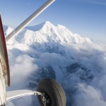
Figure \(\PageIndex{1}\) shows the rugged terrain one finds in the Front Range of the Colorado Rocky Mountains. North is at the top of the photograph. Alpine glaciers are found in favorable sites for snow and ice accumulation. Few of these glaciers are very active under present day conditions though. The glacier is easily identified by its white color. Surrounding the glacier on its western, southern, and eastern sides are the walls of a cirque in which it sits. A cirque is a bowl-shaped landscape feature common to mountainous regions which have been glaciated. The glacier formed in the area to the bottom of the picture and extended itself towards the north. The dark triangular - shaped feature to the north of the glacier is Triangle Lake.

Remote Sensing and Satellite Imagery

To get a much larger view of the earth’s surface features, geographers have turned to using remotely sensed data from satellites. Satellite sensors scan the surface and break it down into picture elements or pixels like those displayed on your computer monitor. Each pixel is identified by coordinates known as lines (horizontal rows), and samples (vertical columns). As the satellite scans the ground, it transmits this information to earth-based receivers, the same way a television station broadcasts a signal to your television. The digital data received is processed in a variety of ways: simulated natural color, "false" color, signal filtering, enhanced contrast, etc.

Figure \(\PageIndex{2}\) shows a portion of the Mississippi River that lies north of Vicksburg along the Arkansas-Louisiana-Mississippi state borders. The image was created from data obtained by Spaceborne Imaging Radar – C/X-band Synthetic Aperture imaging system aboard the space shuttle Endeavor. These images help scientists assess flooding potentials and land management along the river. Much of the area in purple is agricultural land. Areas occupied by water appear in black while the bright green areas are forested. The long narrow lakes bordering the river are called oxbow lakes and are created when the river changes course, abandoning the old channel for a new one. NASA has a detailed discussion (optional reading) about imaging radar online. Read how remote sensing is used to evaluate drought, desertification and the effect of war on Mozambique .

• INTERVIEWS WITH ME
• TESTIMONIALS
• DAN’S FLYING BLOG
• ONLINE COURSES
• PERSONAL COACHING
• YOUTUBE TUTORIALS
• UPCOMING EVENTS
• AFFILIATE PROGRAM
• LIGHTING & FLASH GEAR
• LIGHT SHAPING TOOLS
• ACCESSORIES
• MY AMAZON STORE
• LIGHTING GEAR
• CAMERA BAGS
• COMPUTER EQUIPMENT

5  comments

On Assignment: Shooting Aerials of Denali

By   Dan

June 28, 2010

I was recently hired by Story Worldwide to shoot photos for an article in Holland America’s Mariner Magazine they are running about Denali National Park, with the emphasis on getting a great aerial shot of Denali (Mt. McKinley) for the cover.

After discussing specifics and time frames, I started tracking the weather, which can be extremely finicky in the summertime. One statistic I saw showed that the mountain is only visible for an average of four days in the month of June. Denali rises so high above the surrounding landscape that it literally makes its own weather. Wind currents hitting the sides of the mountain area forced upwards, and in the process the air cools and condenses into clouds. Since warm air holds more moisture than cold air, there are just way more clouds that surround the mountain in the summer.

Spotting a short but promising window of opportunity last weekend, I drove up to the park entrance, caught a camper bus out to Kantishna and parked myself out there a the west end of the park until the weather cleared. I spent three days day hiking in the park, tromping around the tundra and hoofing it up and down the wide open gravel river bars, all the while capturing landscapes and animal shots for the article.

Eventually, on Sunday evening, after a day of building moisture and towering cumulous clouds, the sky let loose with all its moisture. By 8:00PM, the mountain came out and revealed itself in all it’s grandeur. I caught the bus back to Kantishna and scheduled an air taxi flight for 10:00PM. Shoot on!

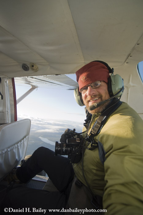
We went down to the airstrip, where they were prepping the Cessna 206 for the photo flight and removing both passenger doors for maximum visibility and clarity. With me in the back seat secured by seat belt that was duct taped closed for added safety, we took off underneath a rainbow from the clearing storm, turned south and climbed to nearly 13,000 feet.

For the next hour, the pilot made circles and followed my direction as I looked for the best angles and shot aerials of Denali and the rest of the Alaska Range out of the open door. I used a Nikon D700 and a D300, with 17mm, 24mm and 50mm lenses. Above 10,000 feet, the late evening sky was perfectly clear and the moon was out, making for near perfect photography conditions. The only thing that would have made it better would have been to take off two hours later in order to get the best evening light. However, due to pilot duty hour regulations, this wasn’t possible, since my pilot had been flying since early that morning.

Overall, the assignment went off without a hitch, except that on my way out of the park on Tuesday morning, my shuttle bus drove off without me at one of the rest stops. Of course, my packs and all my camera gear (and full memory cards!) were still on the bus, and after I managed to catch a new bus, it took me the rest of the day to track down all of my stuff.

Very special thanks to all the great folks at Kantishna Air Taxi and the Skyline Lodge- great pilots, great people and a wonderful place to stay. I highly recommend them for lodging and/or flightseeing on the North side of the Park.

Edit- 10/25/10: The issue has been published, you can see my photo on the cover here.

About the author

Hi, I'm Dan Bailey, a 25+ year pro outdoor and adventure photographer, and official FUJIFILM X-Photographer based in Anchorage, Alaska.

As a top rated blogger and author my goal is to help you become a better, more confident and competent photographer, so that you can have as much fun and creative enjoyment as I do.

New Book – FUJIFILM X SERIES UNLIMITED, 2nd Edition

Dxo photolab 6 now has full fujifilm x-trans support, read student testimonials for my fujifilm autofocus course, new online course – mastering the fujifilm autofocus system, my first photos shot with the fujifilm x-t5, the fujifilm x-t5 is here, check out my brand new online photography school, my bestselling fujifilm guide now covers the x-h2 and x-h2s.

cool gig! how do I get to be a famous adventure photographer like you? weren’t you worried about that seat belt? At first I thought the 10 PM start must be a typo, but I get it now. endless days!

some great images. have they decided which they will use?

Dan, The misty mountain magic that engulfs that big rock is a wonder in itself. I’ve done that flightseeing trip, and it is spectacular. Kudos to you for paying the dues for waiting out and targeting the right weather. Are you going to show us a few of your favorite shots from the shoot or are they locked up until after publication? Additionally, besides your self portrait with the 17mm, did you not find that way too wide to shoot with? Oh, I forgot, some of those cameras may not be full frame. Additionally, I’m surprised you did not have a longer lens to pick up some detail shots of the mountain ridges, or was this not in the desired scope? And finally, I’m happy to hear there are a few thrilling assignments circulating out there…

Patrick, I mostly shot medium to wide shots, as the focus on the assignment was to get a cover worthy aerial shot of the entire mountain, or as much of it as possible. With limited time in the flight, that’s about all I had time for. The wide angles actually did quite well, and with the D300 and D700 I had a thorough variety of focal length/magnifications to choose from. Photos to follow after initial publication by the client. Yes, it’s a good sign indeed that there is work like this out there, I’m hoping that more comes along as the year progresses!

This is awesome Dan! What a priviledge!

[…] another great new client, Holland America and their media company, Story Worldwide, hired me to photograph the cover story about Denali for Mariner Magazine. In addition to getting landscape and wildlife shots, I got to shoot aerials of Denali (Mt. […]

Never miss a post!

 Subscribe and get notified whenever I write something new!

Session expired

Please log in again. The login page will open in a new tab. After logging in you can close it and return to this page.

Aerial Photography

GIS Development Staff

Science and technology must play a key role in formulating the national disaster management

Policy of a country An aerial photograph presents a “bird’s-eye view” of the features on the ground as seen from the air. They are different from ordinary photographs as they present an aerial view of the objects i.e. objects are portrayed from an overhead position. These photographs are also recorded in infra-red wavelengths of light. Although both maps and aerial photos present a “bird’s-eye” view of the earth, aerial photographs are NOT maps. Maps are orthogonal representations of the earth’s surface, meaning that they are directionally and geometrically accurate (at least within the limitations imposed by projecting a 3-dimensional object onto 2 dimensions). Aerial photos, on the other hand, display a high degree of radial distortion. That is, the topography is distorted, and until corrections are made for the distortion, measurements made from a photograph are not accurate. Nevertheless, aerial photography is a powerful tool for studying the earth’s environment.

The history of aerial photography dates back to 1858, when Nadar took photographs of the ground from a rising balloon. During World War I, aerial photography became recognised as an operational military reconnaissance tool and airplanes photographed enemy territories and movements. After the war, the potential use of this technology for civilian purposes was acknowledged and it began to be used for making maps, retrieving information regarding the topography, landform, vegetation and cultural features present on the surface of the earth. Since then, countries have been photographing their areas on a regular basis, both for military and civilian purposes. With the advance in technology, better instruments began to be used for obtaining good quality photographic data. Soon remote sensing satellites came into picture, which could also provide good quality data in a repetitive cycle and the data was available at much cheaper price than their counterparts. Because of this technology, the importance of aerial photography began to be questioned. The scenario is fast changing now. As most of the world has been mapped at scales of 1:50,000 and some even less, the demand for higher resolution photographs is increasing day by day for mapping areas at much smaller scales. This increase corresponds to the rapid increase in industrial and urban development. In this respect aerial photography is proving to be a boon as it can provide us with very high-resolution photographs with ease. Some aspects of aerial photography are covered below.

Catching a view In aerial photography the photographs are taken in “runs” in the direction of flight in such a way that there is approximately 60% overlap between adjacent photographs. The plane is flown in such a way that there is 30% sidelap between adjacent runs. Aerial photographs are classified on the basis of orientation of the camera axis: Vertical Aerial Photography and Oblique Aerial Photography; on the basis of the lens system: Single lens photography, Trimetrogon (Three lens photography), Continuous strip photography and on the basis of films, filters and equipment: Black and white (panchromatic) photography, colour photography, colour infra-red photography etc. Vertical Aerial Photographs are taken with the camera axis pointing vertically down or nearly so at the time of exposure, whereas Oblique Aerial Photographs are taken with the camera axis inclined with respect to the vertical. In panchromatic photography, the film is exposed through minus blue or yellow colour permitting the recording of wavelengths from only parts of the visible range of the spectrum. This type of photography is most suited to general photo interpretation. Infra-red photography records wavelengths of only red and infra-red part of the visible spectrum and is best suited for forest studies and for water vegetation discrimination. Similarly, colour infra-red photography records spectral colours and infra-red in combination resulting in false colours. This type of photography is helpful in vegetation studies related with discrimination of plants and crops etc.

Geometry of Photography Photogrammetry is a science in which the aerial photographs serve the basis for the making reliable measurements for preparation of maps, digital elevation models etc. A few features of photogrammetric operations are listed below:

• Helps in determination of horizontal ground distances and angles made from measurements on a photograph.
• Relief displacements and measurement of image parallax help in determination of object heights.
• Helps in preparation of maps in stereoplotters.
• Based on the above, preparation of digital elevation models and orthophotographs.

Mapping the photograph Photogrammetric procedures are utilised for the preparation of maps. In the aerial photographs certain ground control points are identified. The precise geographic location of such points is then found out. In ideal case there should be at least three such marked points on ground in each aerial photograph. With the help of such three points, the locations of all the other points are determined. The points identified on the photograph are transferred to a base map of suitable scale and projection. The plotted points on the photograph are pin pricked and positioned in a plotting machine and adjusted for scale, tilt and other distortions until the points on the photograph and the base map coincide. Thus, an accurate model of the terrain is recreated. This whole procedure is carried out on a stereoplotting machine. The created model can be viewed stereoscopically and used to create a planimetric map having no relief distortions. Topographic contours can also be plotted on the map as the height of the features on the model can be easily determined and transferred onto the map.

Digital Methods in Aerial Photography Although the photographs provide an excellent resolution, in today’s digital world, the analogue data is of little use until it is processed and converted into digital form. Digital data has many advantages as the data can be processed with ease, enhanced, analysed and presented in an easily understandable form through the application of computers. In photogrammetry, aerial photographs are utilised to form a three-dimensional model which when further processed can yield mapping data. This process involves the usage of computers and thus it is beneficial to store the raw data in the a digital format so that each image point (pixel) can be distinguished in terms of its position and brightness level. The most important advantage of data in a digital format is that it can be directly utilised for analysis in a GIS environment. There are two different approaches to obtain aerial photographs in digital format (a) scanning of existing aerial photograph and (b) direct digital acquisition. Existing aerial photographs can be scanned using scanner. In this process the aerial photograph is scanned by either moving the charge coupled device (CCD) sensor head over the photo or moving the photo carriage over a static sensor. Once the image is scanned, the digital form of the image can be easily imported to a software where the data can be processed for GIS or remote sensing application. The recent trend in digital aerial photography is the use of digital cameras. Although still in its early stages, this technology will prove to be a major breakthrough in the field of aerial photography. Digital cameras use the CCD technology in which the patterns of blacks, greys and whites are electronically recorded as digital values, each representing the brightness of a specific point within the image. The main advantage of this technology includes its size, weight, dynamic range, optical sensitivity, stability, linearity and durability. Currently, the major disadvantages of this technology are its exorbitant price and the limited size of the CCD sensor array which can be used only for small format applications.

Using GPS to enhance Aerial Photography Knowledge of exact locations of several features on the surface of the earth helps in registration of the photograph. Registration of a photograph means that a coordinate system can be overlaid on the photograph such that location of each feature on the photograph can be represented by a set of co-ordinate points. Prior to registration, the exact coordinates of the features that are seen on a photograph are determined by surveying techniques. Enough targets must be placed to ensure that a sufficient number of them (usually three or more) appear in each photograph. The role of GPS comes in the exact location of features on the ground. Recent advances in handheld Global Positioning System (GPS) receivers have made the task of precisely locating features fast, easy, and inexpensive.

Earlier the use of GPS receivers for registration of features on photograph was not advised as it would provide inaccurate results, correct to only 100 meters, which could be corrected upto 10 meters using correction algorithms. However, recently GPS receivers have been prepared which are accurate within a few centimetres. The data provided by the GPS requires post-processing on a computer before it can be used, but this once-difficult procedure has become much simpler now. So to obtain adequate ground control, we only have to select a number of naturally occurring features on the ground and acquire GPS positions for them. Once the photographs are registered then they “fit” within some standard coordinate system such as latitude/longitude or Universal Transverse Mercator (UTM).

The above method works very well when the photographed area is easily accessible. However, large areas like dense forests, steep hills etc. are not accessible. If these areas have to be covered by an aerial photo then the process of photo registration is not very accurate. It is only possible to approximately register such a photograph in the absence of traditional ground control. This is possible if the camera’s position and orientation (latitude, longitude, and direction of travel) are known at the time the photograph is taken. Modern GPS receivers can help in recording such information so that data having accuracy within 100 meters is saved and is transferred to a computer for correction such that the corrected data accurate to within 2 to 5 meters is obtained.

In order to register such photographs, the flight path along with the exact time the photograph is taken is recorded. The record of the exact time each photo is taken helps to find the corresponding inflight position. A system is developed such that each time a photo is taken, a GPS records position and time data.

After the flight, the record of the complete flight path along with the times each photo was taken is exported to a computer and subsequent processing and differential correction of the flight path data gives out data having an accuracy of 2-5 meters. Then the two datasets are merged to provide the position data for each photograph.

GIS Database with Aerial Photographs Each point in a digital aerial photograph represents a geographic location with a characteristic value associated with it. This information forms the basis of the geographic data related with the point. A collection of such data for all the associated points in the aerial photograph results in a database that can be used for analysis of the photograph in a GIS environment. Registered photographs can be incorporated into a geographic information system (GIS) and used to create or update maps. Aerial Photographs which are not digital, require manual scanning of the photograph. Once the photograph is scanned, it results in a digital image. But this image does not represent any data as it is just a collection of pixels of varying values. To define the data present in the digital image, either photogrammetric operations are carried out or the photograph undergoes digitisation process. Both these operations provide the image a well-defined data structure wherein each point provides attribute as well as spatial data associated with the point. Once such a database forms, GIS operations can be undertaken for analysis work related to the area represented by the image.

Recent Trends in Aerial Photography

Small Format Aerial Photography Except a very few areas, aerial photography of most of the parts of the earth have been carried. With the advent of satellite remote sensing, even these areas have been covered. With rapid urbanisation and industrialisation the need of the hour is very high resolution maps i.e. large scale maps. In this respect small format aerial photography is playing a key role. In this type of photography a small format (35mm) automatic camera is used. This type of camera allows for hands-free operation and is light enough to be lifted by a large kite. Critical camera settings like focus, shutter speed etc. are controlled by a microchip and light meter within the camera body. Simple acquisition of airphotos can be attained by enabling the camera’s timer function to take photograph after a few seconds.

Low Altitude Remotely Piloted Vehicle (RPV) Aerial Photography The latest improvement in aerial photography is the utilisation of a remotely piloted vehicle (RPV) for aerial photography. Utilizing an unmanned, remotely piloted vehicle, offers cost effective alternatives to traditional aerial photography. Since RPV’s are not limited by the same restrictions as full-size aircraft, they can be operated at altitudes of less than 500 feet, even in residential areas where full-size aircraft are restricted to a minimum altitude of 1000 feet. As a result of the freedom associated with this method of aerial photography unique, low cost aerial photographs from previously impossible perspectives for a multitude of applications can be obtained.

RELATED ARTICLES MORE FROM AUTHOR

The making of Jack Dangermond: Godfather of GIS

Why You Need Location Intelligence for 5G Deployment Success

Sustainability of everything

© Geospatial Media and Communications. All Rights Reserved.​

Table of Contents

Introduction To Aerial Photographs  

We   are familiar with photographs taken with normal cameras. These photographs provide us with a view of the object similar to the way we see them with our own eyes. In other words, we get a horizontal perspective of the objects photographed. For example, a photograph of a part of settlement will provide us a perspective the way it appears to us when we look at it (Fig. 6.1).

Figure 6.1 Terrestrial photograph of Mussorrie town

Suppose we want to take a ‘bird’s eye view’ of similar features, then we have to place ourselves somewhere in the air. When we do so and look down, we get a very different perspective. This perspective, which we get in aerial photographs, is termed as aerial perspective (Fig. 6.2).

Figure 6.2 Bird’s Eye View of Tehri Town, Uttarakhand

The photographs taken from an aircraft or helicopter using a precision camera are termed aerial photographs . The photographs so obtained have been found to be indispensable tools in the topographical mapping and interpretation of the images of the objects.

Aerial Camera : A precision camera specifically designed for use in aircrafts.

Aerial Film : A roll film with high sensitivity, high intrinsic resolution power and dimensionally stable emulsion support.

Aerial Photography : Art, science and technology of taking aerial photographs from an air-borne platform.

Aerial Photograph : A photograph taken from an air-borne platform using a precision camera.

Fiducial Marks : Index marks, rigidly connected at the central or corner edges of the camera body. When the film is exposed, these marks appear on the film negative .

Forward Overlap : The common area on two successive photographs in the flight direction. It is usually expressed in per cent.

Image Interpretation : An act of identifying the images of the objects and judging their relative significance.

Nadir Point : The foot of the perpendicular drawn from the camera lens centre on the ground plane.

Principal Point : The foot of the perpendicular drawn from the camera lens centre on the photo plane.

Principal Distance : The perpendicular distance from the perspective centre to the plane of the photograph.

Perspective Centre : The point of origin (perspective centre) of the bundle of light rays.

Photogrammetry : The science and technology of taking reliable measurements from aerial photographs.

Uses of Aerial Photographs

Aerial photographs are used in topographical mapping and interpretation. These two different uses have led to the development of photogrammetry and photo/image interpretation as two independent but related sciences.

Photogrammetry: It refers to the science and technology of making reliable measurements from aerial photographs. The principles used in photogrammetry facilitate precise measurements related to the length, breadth and height from such photographs. Hence, they are used as the data source for creating and updating topographic maps.

The development of aerial photography in India is briefly given in Box 6.I.

Box 6.1 Aerial Photography in India

Aerial photography in India goes back to 1920 when large-scale aerial photographs of Agra city were obtained. Subsequently, Air Survey Party of the Survey of India took up aerial survey of Irrawaddy Delta forests,

which    was completed during 1923–24. Subsequently, several similar surveys were carried out and advanced methods of mapping from aerial photographs were used. Today, aerial photography in India is carried out for the entire country under the overall supervision of the Directorate of Air Survey (Survey of India) New Delhi. Three flying agencies, i.e. Indian Air Force, Air Survey Company, Kolkata and National Remote Sensing Agency, Hyderabad have been officially authorised to take aerial photographs in India.

The procedure for indenting aerial photographs for educational purposes could be made with APFPS Party No. 73, Directorate of Air Survey, Survey of India, West Block IV, R. K. Puram, New Delhi.

Image Interpretation: It is an art of identifying images of objects and judging their relative significance. The principles of image interpretation are applied to obtain qualitative information from the aerial photographs such as land use/land cover, topographical forms, soil types, etc. A trained interpreter can thus utilise aerial photographs to analyse the land-use changes.

Advantages of Aerial Photography

The basic advantages that aerial photographs offer over ground based observation are :

a. Improved vantage point : Aerial photography provides a bird’s eye view of large areas, enabling us to see features of the earth surface in their spatial context.

b. Time freezing ability: An aerial photograph is a record of the surface features at an instance of exposure. It can, therefore, be used as a historical record.

c. Broadened Sensitivity: The sensitivity of the film used in taking aerial photographs is relatively more than the sensitivity of the human eyes. Our eyes perceive only in the visible region of the electromagnetic spectrum, i.e. 0.4 to 0.7 µm whereas the sensitivity of the film ranges from 0.3 to 0.9 µm.  

d.  Three   d imensional   p erspective: Aerial photographs are normally taken with uniform exposure interval that enables us in obtaining stereo pair of photographs. Such a pair of photographs helps us in gett ing a three-dimensional view of the surface photographed.

Types of Aerial Photographs

The aerial p hotographs are classified on the basis of the position of the camera axis, scale, angular extent of coverage and the film used. The types of the aerial photographs based on the position of optical axis and the scale are given below : d.

a. Types of Aerial Photographs Based on the Position of the Cameral Axis: On the basis of the position of the camera axis, aerial photographs are classified into the following types :

(i) Vertical photographs

(ii) Low oblique photographs

(iii) High oblique photographs

(i) Vertical Photographs: While taking aerial photographs, two distinct axes are formed from the camera lens centre, one towards the ground plane and the other towards the photo plane. The perpendicular dropped from the camera lens centre to the ground plane is termed as the vertical axis, whereas the plumb line drawn from the lens centre to the photo plane is known as the photographic/optical axis . When the photo plane is kept parallel to the ground plane, the two axes also coincide with each other. The photograph so obtained is known as vertical aerial photograph (Figures 6.3 and 6.4).

 However, it is normally very difficult to achieve perfect parallelism between the two planes due to the fact that the aircraft flies over the curved surface of the earth. The photographic axis, therefore, deviates from the vertical axis. If such a deviation is within the range of plus or minus 3 o , the near-vertical aerial photographs are obtained. Any photography with an unintentional deviation of more than 3 o in the optical axis from the vertical axis is known as a tilted photograph.  

(ii) Low Oblique: An aerial photograph taken with an intentional deviation of 15° to 30° in the camera axis from the vertical axis is referred to as the low oblique photograph (Figures 6.5 and 6.6). This kind of photograph is often used in reconnaissance surveys.

(iii) High Oblique:   The high oblique are photographs obtained when the camera axis is intentionally inclined about 60° from the vertical axis (Figure 6.7). Such photography is useful in reconnaissance surveys.

Figure 6.7 High Oblique Photograph

 Table 6.1 provides a comparison between vertical and oblique photographs.

b) Types of Aerial Photographs Based on Scale: The aerial photographs may also be classified on the basis of the scale of photograph into three types.

(i) Large Scale Photographs : When the scale of an aerial photograph is 1 : 15,000 and larger, the photography is classified as large-scale photograph (Fig. 6.8).

Figure 6.8 1 : 5000 Photograph of Arnehem

(ii) Medium Scale Photographs: The aerial photographs with a scale ranging between 1 : 15,000 and 1 : 30,000 are usually treated as medium scale photographs (Fig. 6.9).

   Figure 6.9 1 : 20,000 Photograph of Arnehem

(iii) Small Scale Photographs:  The photographs with the scale being smaller than 1 : 30,000, are referred to as small scale photographs (Fig. 6.10).

Figure 6.10 1 : 40,000 Photograph of Arnehem  

Geometry of an aerial photograph.

To understand the geometry of an aerial photograph, it is important to appreciate the orientation of the photograph with respect to the ground, i.e. the way the rays connect or ‘project’ onto the ground in relation to the ground representation (photograph or map). The following three examples of such projection would be useful in understanding the problem.

Parallel Projection: In this projection, the projecting rays are parallel but not necessarily perpendicular. The triangle ABC is projected on LL1 as triangle abc ( f igure 6.11).

  Figure 6.11 Parallel Projection

Orthogonal   P rojection: This is a special case of parallel projections. Maps are orthogonal projections of the ground. The advantage of this projection is that the distances, angles or areas on the plane are independent of the elevation differences of the objects. Figure 6.12 is an example of orthogonal projection where the projecting rays are perpendicular to the line LL1.  

  Figure 6.12 Orthogonal projection

Central Projection: Figure 6.13 shows an example of Central Projection. The projecting rays Aa, Bb and Cc pass through a common point O, which is called the perspective Centre. The image projected by a lens is treated like a central projection.

Figure 6.13 Central Projection

An aerial photograph, as discussed earlier is a central projection. In an absolutely vertical flat terrain the aerial photograph will be geometrically the same as the corresponding map of the area. However, because of the tilt of the photograph and relief variations of the ground photographed, an aerial photograph differs geometrically from the map of the corresponding area. 

As shown in Figure 6.14, S is the camera lens centre. The bundle of light rays coming from the ground plane converge at this point and diverge from there towards the negative (photo) plane to form images of the objects. Thus, the central projection is characterised by the fact that all straight lines joining corresponding points, i.e. straight lines joining object points to their corresponding image points pass through one point. Figure 6.14 illustrates this relationship. Straight lines AAi, BBi, CCi and DDi join corresponding points on the ground photographed and the negative plane. For example, A on the ground and Ai on the negative plane (or ‘a’ on the positive plane) is a line joining corresponding points which pass through the camera lens centre. If we draw a perpendicular from S following the camera axis onto the negative plane, the point where this perpendicular meets the negative is known as the principal point (P in Fig. 6.14). If we extend the same line to the ground, it would meet the target (photographed ground) plane at PG, i.e. the ground principal point. Similarly, if we draw a vertical line (plumb line as indicated by the direction of gravity) through S, it will meet the photo negative at a point known as the nadir point and on the ground as the ground nadir point. Observe from figures 6.3, 6.5 and 6.7 that the plumb line and the camera axis are coincident for a vertical photograph while they are separable in case of an oblique or a tilted photograph. Thus in case of a vertical photograph, the principal and the nadir points also coincide with one another. For an oblique photograph, the angle between the camera axis and the plumb line is the tilt angle. Figure 6.14 shows both the positive and the negative planes of a vertical photograph. The geometry of the positive a nd the negative planes are identical.

Figure 6.14 Geometry of Vertical Photograph

It ne eds to be understood here that SP, i.e. the perpendicular distance between the camera lens and the negative plane is known as the focal length. On the other hand, SP G , i.e., the perpendicular distance between the camera lens and the ground photographed is known as the flying height

Difference between a Map and an Aerial Photograph

A map cannot be directly traced out of an aerial photograph. The reason is that there is a basic difference in the planimetry (projection) and perspective of a map and an aerial photograph. The difference is given in Table 6.2.

Even vertical aerial photographs do not have a consistent scale unless they have been taken of a flat terrain. Aerial photographs need to be transformed from perspective view to the planimetric view before they can be used as map substitute. Such transformed photographs are known as orthophotos .

Scale of Aerial Photograph

You are already familiar with the concept of a map scale (See Chapter 2). The concept of scale for aerial photographs is much the same as that of a map. Scale is the ratio of a distance on an aerial photograph the distance between the same two places on the ground in the real world. It can be expressed in unit equivalents like 1 cm= 1,000 km(or 12,000 inches) or as a representative fraction (1:100,000). 

Scale determines what objects would be visible, the accuracy of estimates and how certain features will appear. When conducting an analysis that is based on air photos, it will sometimes be necessary to make estimates regarding the number of objects, the area covered by a certain amount of material or it may be possible to identify certain features based on their length. To determine this dimension during air photo interpretation, it will be necessary to make estimates of lengths and areas, which require knowledge of the photo scale. There are three methods to compute the scale of an aerial photograph using different sets of information.

Method 1: By Establishing Relationship   b etween Photo Distance and Ground Distance : If additional information like ground distances of two identifiable points in an aerial photograph is available, it is fairly simple to work out the scale of a vertical photograph. Provided that the corresponding ground distances (D g ) are known for which the distances on an aerial photograph (D p ) are measured. i n such cases, the scale of an aerial photograph will be measured as a ratio of the two, i.e. D p / D g .

Problem 6.1 The distance between two points on an aerial photograph is measured as 2 centimetres. The known distance between the same two points on the ground is 1 km. Compute the scale of the aerial photograph (Sp).

Sp = D p : Dg

= 2 cm : 1 km

= 2cm : 1 x 100,000 cm

= 1 : 100,000/2 = 50,000 cm

= 1 unit represents 50,000 units

Therefore, Sp = 1 : 50,000

Method 2: By Establishing Relationship   b etween Photo Distance and Map Distance: As we know, the distances between different points on the ground are not always known. However, if a reliable map is available for the area shown on an aerial photograph, it can be used to determine the photo scale. In other words, the distances between two points identifiable both on a map and the aerial photograph enable us to compute the scale of the aerial photograph (Sp). The relationship between the two distances may be expressed as under :

( Photo scale : Map scale) = (Photo distance : Map distance)

We can derive

Photo scale (S p ) = Photo distance (D p ) : Map distance (D m ) x Map scale factor (msf)

Problem 6.2 The distance measured between two points on a map is 2 cm. The corresponding distance on an aerial photograph is 10 cm. Calculate the scale of the photograph when the scale of the map is 1: 50,000.

Sp = D p : Dm x msf

Or = 10 cm : 2 cm x 50,000

Or = 10 cm : 100,000 cm

Or = 1 : 100,000/10 = 10,000 cm

Or = 1 unit represents 10,000 units

Therefore, Sp = 1 : 10,000

Method 3: By Establishing Relationship   b etween Focal Length (f) and Flying Height (H) of the Aircraft : If no additional information is available about the relative distances on photograph and ground/map, we can determine the photo-scale provided the information about the focal length of the camera (f) and the flying height of the aircraft (H) are known (Fig. 6.15). The photo scale so determined could be more reliable if the given aerial photograph is truly vertical or near vertical and the terrain photographed is flat. The focal length of the camera (f) and the flying height of the aircraft (H) are provided as marginal information on most of the vertical photographs (Box 6.2).

Figure 6.15 Focal Length of the Camera (f) and Flying Height of the Aircraft (H)

The Fig. 6.15 may be used to derive the photo-scale formula in the following way :

Focal Length (f) : Flying Height(H) =

Photo distance (Dp) : Ground distance (Dg)

Problem 6.3 Compute the scale of an aerial photograph when the flying height of the aircraft is 7500m and the focal length of the camera is 15cm.

Or Sp = 15 cm : 7,500 x 100 cm

Or Sp = 1 : 750,000/15

* 793 is a Photo Specification number maintained by the 73 APFPS Party of the Survey of India. B is the Flying Agency that carried out the present photography (In India three flying agencies are officially permitted to carry out aerial photography. They are the Indian Air Force, the Air Survey Company, Kolkata and the National Remote Sensing Agency, Hydrabad, identified on the aerial photographs as A, B and C respectively), 5 is the strip number and 23 is the photo number in strip 5.

Multiple Choice Questions

1. In which of the following aerial photographs the horizon appears?

a. Vertical

b. Near-vertical

c. Low-oblique

d. H igh-oblique

2. In whic h of the following aerial photographs the Nadir and the principle points coincide?

d. Hi gh-oblique

3. Which type of the following projections is used in aerial photographs?

a. Parallel

b. Orthogonal

d. No ne of the above.

Short Questions  

1. State any three advantages that an aerial photograph offers over ground based ob servations.

2. How is an aerial photograph taken?

 3. Present a concise account of aerial photography in India.

  4. Answer the follow ing questions in about 125 words :

i) What are the two major uses of an aerial photograph? Elaborate.

ii) What are the different methods of scale determination?

Photo Assignment: From the Sky

A whole new perspective on photography.

A drone is just a camera with wings. Or propellers, I guess. Just like, to a cat, a bird is just a mouse with wings. It’s all your perspective.

And yes, I now have a drone. It’s been about six or seven weeks since I bought the device and four weeks since I passed my FAA Part 107 UAS (Unmanned Aircraft System) exam, which means I’m now a licensed drone photographer. Without going too deep, the reason I did this was that, as a real estate photographer, when a real estate agent wants aerial photography or video, I had to hire a friend of mine, Tony, who is a great guy and a terrific drone pilot. But it meant I made no money off of his services, and I wasn’t having the fun he was by flying his drone around, snapping off photos from the sky.

I knew this was coming, and I’m glad it’s here. Since I received my UAS certificate, I’ve done several real estate photoshoots that included drone shots. Some of them were part of the job, and others I just included to expand my flying experience.

Mixed Tape: Pulses, Prose, and Pix is a reader-supported publication. To receive new posts and support my work, consider becoming a free or paid subscriber.

That’s all good and well, but to me, the real fun of being a drone photographer is the world that having a flying camera opens up. It’s an entirely new perspective on taking photos and videos, and it’s fun.

One thing I’ve heard among drone pilots is not “if” you crash your drone, but “when.” So far, so good! I haven’t crashed and haven’t even had any close calls. But this post isn’t about the drone or the rules of flying or FAA-regulated airspace. It’s more about some of the images I’ve captured in the last few weeks.

Let’s start with this one: I headed out east of Salem to see what I could find and came across the Gilkey Covered Bridge. Oregon is home to dozens of these old bridges, and this was a great opportunity to explore with my winged camera a bit:

Share Mixed Tape: Pulses, Prose, and Pix

But to back up a bit, the very first place I flew the drone was in Keizer Rapids Park. I have to say it was exhilarating to put that little DJI Mini 4 Pro in the air for the first time:

My next stop a few days later was east of Salem over some farmland, where I came across an old cemetery:

Back in Salem, I took the flying lens to Riverfront Park:

The weekend after Mother’s Day, I was camping with friends at a cool campground on the Deschutes River on the Warm Springs Reservation in central Oregon, so of course, I got up early to take some images:

To close out this week’s post, a bit on the video capabilities of the drone, which can do programmed shoots based on some damn sophisticated software. For example, in one program, it takes what it calls “hyper-lapse” images, and then assembles the images into a short movie. Timelapse, basically. And the drone stays in place while it snaps the images. This 17-second video took 17 minutes to capture as it took a frame every two seconds. I purposely timed this so it would catch the rays of the rising sun coming over the ridge, illuminating the treetops. I got lucky with some unexpected visitors at the very end:

This week, while shooting some aerial videos and stills for a client, I realized that I’ve made a lot of progress in a very short time. My comfort zone while flying the drone has increased dramatically, my array of shots and videos is more thorough and better, and I imagine it will only get better from here.

Loads of fun, no doubt, you’ll see more of my aerial photography in the future!

Ready for more?

• Increase Font Size

13 Aerial Photography

Dr. Puneeta Pandey

1.  Aim of the Module

2.  Introduction

3.  History of Aerial Photography

4.  Commercial Aerial Photography

5.  Basic concepts of Aerial Photography

6.  Types of Aerial Photography

7.  Types of Film

8.  Applications of Aerial Photography

9.  Advantages of Aerial Photography over ground-based observation

10.  Conclusion

11.  References

• To understand the basic concept of Aerial Photography To study the history of Aerial Photography
• To study the applications and advantages of Aerial Photography

Aerial photography is the process of capturing of photographs of features of the earth’s surface from a certain height or an elevated position using high resolution camera mounted on platforms like helicopters and other light aircrafts which include fixed-wing aircraft, balloons, drones, blimps and dirigibles, pigeons, rockets, kites, vehicle-mounted poles and parachutes. The mounted cameras may be triggered automatically or remotely; hand-held photographs may be taken by a photographer. There are certain things taken into consideration while dealing with fundamental understanding of aerial photography which include scale, film, focal length, overlap, stereoscopic coverage, fiducial marks, roll and frame numbers, and flight lines and index maps.

Figure 1: Antique postcard using kite photo technique (circa 1911) (http://www.wikiwand.com).

Figure 2: Giza pyramid complex, photographed from Eduard Spelterini’s balloon on Nov. 21, 1904 (http://www.commons.wikimedia.org).

Figure 3: A German observation plane, the Rumpler Taube (http://www.en.wikipedia.org).

Figure 4: A drone carrying a camera for aerial photography (http://www.en.wikipedia.org).

Figure 5: A camera is attached to pigeon for capturing of aerial photos

(http://www.northstargallery.com).

3. History of Aerial Photography

The first known aerial photograph was first practiced in 1858 over Paris, France by the French photographer and balloonist G. F. Tournachon, known as “Nadar”. The landscape captured by the photograph was of the French village of Petit-Becetre taken at 80m from ground using a tethered hot-air balloon. However, the photographs did not survive for long and therefore the oldest existing aerial photograph is titled “Boston, as the Eagle and the Wild Goose See It”, depicts Boston from an altitude of 630m, captured by J. W. Black and S. A. King on October 13, 1860 (Figure 6). In addition hot air balloons, pigeons, kites and rockets are also used to carry the cameras in the air to capture the photographs. Aerial photograph from a rocket mounted camera was taken for the first time by the  Swedish inventor, Alfred Nobel in 1897. From an aeroplane, the first successful aerial photography was taken in 1909, by Wilbur Wright.

Figure 6: Balloon view of Boston captured by J. W. Black and S. A. King on October 13, 1860 (https:// www.smithsonianmag.com/…/this-picture-of-boston-circa-1860)

The famous english meteorologist E.D. Archibald initiated Kite aerial photography in 1882 with the help of an explosive charge on a timer to capture successful photographs from the air. On April 24, 1909, the first ever use of a motion picture camera was mounted on an aircraft over Rome in the 3:28 silent film short, Wilbur Wright und seine Flugmaschine .

The use of aerial photography rapidly developed during the war, as aircrafts were equipped with cameras to verify and record enemy movements and defense systems. In 1913, Germany adopted the first aerial camera, a Gorz. The French army began the war with numerous squadrons of Bleriot observation aircraft laden with cameras for survey and also developed procedures for acquiring print out in record time into the hands of field commanders.

In 1915, C. J. Moore-Brabazon invented the first purpose-built and practical aerial camera aided by the Thornton-Pickard company, greatly enhancing the efficiency of aerial photography. Moore-Brabazon also introduced the inclusion of stereoscopic techniques into aerial photography, permitting the height of objects to be differentiated on the landscape by comparing photographs taken at different angles.

4. Commercial aerial photography

Francis Wills and Claude Graham White the World War I veterans, founded the first commercial aerial photography company in the UK was Aerofilms Ltd., in 1919. Later on, the Aircraft Manufacturing Company (the De Havilland Aircraft Company), hired an Airco DH.9 along with pilot entrepreneur Alan Cobham. Another successful breakthrough in commercial aerial photography was given by the American Sherman Fairchild who started his own aircraft firm Fairchild Aircraft in 1935, especially for the purpose of aerial survey missions. Later on, Fairchild developed a high altitude camera with nine-lens in one unit that could capture a photo of 600 sq. miles with each exposure from 30,000 feet. Fairchild also designed and develop airplanes with high-wings and enclosed cabins as a more stable and protected platform for photography that lead to his strong commitment in the business of aerial photography. This aerial map (overlapping photographs) of Manhattan Island became a commercial success of Fairchild which was later on used by several New York City agencies and businesses.

5. Basic Concepts of Aerial Photography

5.1 Camera: In early days the cameras used for photography were often no more than a light-tight box with a pinhole at one end and the exposed light sensitive material fitted against the opposite end. Later on the pinhole camera was replaced by simple lens camera. The Cameras and their applicability for aerial photography are the simplest and oldest of sensors exploited for remote sensing of the earth’s surface. The camera is a framing system which takes a near-instantaneous “snapshot” of an area of the surface. The camera systems are passive optical sensors that use a lens to form an image at the focal plane, the plane at which an image is precisely defined.

5.2 Film: Black and white film are most common films used in aerial photos, however infrared, colour, and false-colour infrared film are also used for certain special projects. The photographic films are sensitive to light from 0.3 μm to 0.9 μm in wavelength which include the ultraviolet (UV), visible, and near-infrared (NIR). Panchromatic films are sensitive to the UV and the visible portions of the spectrum. The panchromatic film is the most common type of film used in aerial photography and produces black and white images.

5.3 Focal length: It is the distance from the middle of the camera lens to the focal plane (i.e. the film) and is calculated after calibration of the camera. With the increase in focal length, image distortion  decreases. The relationship between the focal length (f), object distance (o) and image distance (i) is given below

1/f=1/o+1/i   ——- (Eq. 1)

5.4 Scale: It is the ratio of distance between two points on a photo to the actual distance between the same two points on the ground (i.e. 1 unit on the photo equals “x” units on the ground).

Another method used to verify and evaluate the scale of a photo is to determine the ratio between the camera’s focal length and the plane’s altitude above the ground being filmed.

Unit Equivalent, Representative Fraction and Ratio are some of the ways that can be used to express the scale. For example

A photographic scale of 1 mm on the image represents 25 metres on the ground would be expressed as follows:

Unit Equivalent – 1 mm = 25 m

Representative Fraction – 1/25 000

Ratio – 1:25 000

Scale can be large or small

Large Scale- Larger-scale based photos (e.g. 1: 25,000) cover small regions in greater detail. A large scale photograph means that ground features are expressed in more detailed size at large. The area of ground coverage on the photograph is less than at smaller scales.

Small Scale- the photos that are captured on small scale (e.g. 1: 50,000) cover ground features of large regions/areas in less detail. The area of ground coverage captured on the photo is greater than at larger scales. An example for 1: 50,000 scale is given below-

A variety of photographic scales, such as 1: 3,000 (large scale) of selected areas, and 1: 50,000 (small scale) are available at The National Air Photo Library.

The scale at a point on a truly vertical photograph is given by

S = f/ H- h  ——- (Eq. 2)

S = photographic scale at a point

f = camera focal length

H= flying height above datum

h = elevation above datum of the point

5.5 Exposure: At any point in the image, the exposure is determined by the irradiance at that point multiplied by the exposure time, expressed as

E= sd 2 t/4f 2  ————  (Eq. 3)

E= exposure, J mm-2

s= scene brightness, J mm-2sec-1

d= diameter of lens opening, mm

t= exposure time, sec

f= lens focal length, mm

From the Eq. 2, it can be seen that the exposure varies with respect to shutter speed t and/or the diameter of the lens opening d . The various combinations of d and t will produce equivalent exposures for a given camera.

5.6 Fiducial marks: these are small registration marks (figure 7) that are exposed on the edges of a photograph. The measurement of distances between fiducial marks are precisely is done when a camera is calibrated, and such information is being used during compilation of topographic map by cartographers.

Figure 7: The image showing fiducial marks (http://www.hosting.soonet.ca)

5.7 Overlap: it is the amount by which one photograph comprises the area covered by another photograph, and is expressed as a percentage (%). The photo survey is designed to get 30% lateral overlap (between photos on adjacent flight lines) and 60% forward overlap (between photos along the same flight line)

5.8 Stereoscopic Coverage: It is the representation of the three-dimensional (3D) view which results when two overlapping photos (known as stereo-pair), are viewed with the help of a stereoscope. Each photograph of the stereo-pair offers a slightly different view of the same area, which the brain merges and interprets as a 3-D view.

5.9 Roll and Photo Numbers: It is a type of identification number which allows searching of the photo in NAPL’s archive, besides metadata information, the plane’s altitude, the focal length of the camera, and the weather conditions. Each photograph is assigned a unique index number according to the photo’s roll and frame.

5.10 Flight Lines and Index Maps: the contractor of aerial survey plots the location of the first, last, and every fifth photo centre, along with its roll and frame number, on a National Topographic System (NTS) map. Photo centres are represented by small circles, and straight lines are drawn linking the circles to show photos on the same flight line. This graphical representation is known as air photo index map, which allows the photos to relate with their corresponding geographical location. On NTS map sheets, small-scale photographs are indexed on 1: 250,000 scale, and larger-scale photographs are indexed on 1: 50,000 scale NTS maps.

5.11 Color-Mixing Process: The color mixing is very important for an observer to see the real true colored picture of the landscape. The trichromatic theory of color vision explains that when blue, green and red elements are stimulated by different amount of light, we perceive color just like the phenomenon behind the rod cells and cone cells of the human eye. The red, green and blue are termed as additive primaries whereas yellow, magneta and cyan are known as complementary colors of blue, green and red light. There is a concept called hue cancellation method which states that when the certain colors are mixed together, the resulting colors are not what would be intuitively expected. For example, when red and green are mixed together, the resultant color is yellow not reddish green.

There are two types of color mixing: Additive and Subtractive .

5.11.1 ADDITIVE Mixing: The superimposition of two beams of light corresponds to additive mixing.

The additive mixing of colors is unintuitive as it does not related to the mixing of physical substances which would correspond to subtractive mixing. Regardless of being unintuitive, it is theoretically simpler than subtractive mixing.

In the absence of color, the result is black. If all three primary colors (red, blue and green) are showing, the result is white. When red and green colors are combined, the result is yellow and with that of red and blue, the result is magenta. For blue and green combination, the result is cyan.

Additive mixing is used in television and computer monitors to produce a wide range of colors using only three primary colors. A pixel is a combination of the three primary colors. Projection televisions usually have three projectors, one for each primary color.

5.11.2 SUBTRACTIVE Mixing: The mixing of physical substances corresponds to subtractive color mixing; therefore it corresponds to our perception about mixing colors. To explain the mechanism, let us mix red paint with yellow paint. The red paint is red because when the ambient light strikes it, the composition of the material is such that it absorbs all other colors in the visible spectrum except for red. The red light, not being absorbed, reflects off the paint. The similar mechanism describes the color of all material objects — note that light is not a material object — and so applies to the yellow paint as well.

In subtractive mixing of color, the absence of color is white and the presence of all three primary colors is black. By convention, the three primary colors in subtractive mixing are yellow, magenta and cyan. The secondary colors are the same as the primary colors from additive mixing, and vice versa. Subtractive mixing is used to create a range of colors when printing on paper by combining a small number of ink colors, and also when painting. Upon mixing yellow and blue, Green color is produced and with that of red and yellow, orange is produced.

The color film photography rely on the principle of subtractive color mixture using superimposed yellow, magenta and cyan dyes (Subtractive primaries) to control the proportionate amount of green, blue, and red light that reaches the eye. Therefore, the subtractive mixture of yellow, magenta and cyan dyes on a photograph is used to control the additive mixture of blue, green and red light reaching the observer. To achieve this, color film is manufactured with three emulsion layers that are sensitive to blue, green and red light but contain yellow, magenta and cyan dye after processing.

5.12 Filters: The use of filters or color screens has been very frequent in ordinary landscape photography. With the help of filters a selective wavelength of light reflected from the scene is allowed to reach the image plane (film). They are placed in front of the lens in the optical path of a camera. Filters are often used for the purpose of correct brightness rendering, calculated for a given color sensitive plate so that the resultant feedback to the light of the spectrum copies the sensitiveness of the eye, which is greatest in the yellow-green. Such filters for use with the common orthochromatic plates are of a general yellow color. The filters used in aerial cameras consist of organic dyes suspended in glass or in a dried gelatin film. The most commonly used filters are absorption filters which allows differentiation of objects with nearly similar spectral response patterns in major portions of the photographic spectrum.

ND Filter or neutral density filter is possibly the most useful filter in the aerial photography. This filter is a sunglass lens for the camera, decreasing light levels without altering color or having any other side effects.

The Camera filters are of two types-

Screw-on filters come in different sizes, related to different lenses of the camera. A lens with a 52 mm mount can only work with 55 mm filters.

6. Types of Aerial Photography

6.1 Oblique Aerial Photographs

Oblique photographs are those photographs that are taken at certain angle with respect to the ground surface (ie not directly overhead as in ‘Vertical’). The photographs taken at low angle are known as low oblique photographs whereas those taken at high or steep angle are known as high or steep oblique photographs that include the horizon. Both low and high oblique can be taken as ‘wide shots’ or ‘close-ups’.

Figure 8: Abalone point, Irvine Cove, Laguna Beach an example of low-altitude aerial photography (http://www.sky-photo.net).

Figure 9: Oblique Aerial Photo (http://www.wikiwand.com).

6.2 Vertical Aerial Photographs

Vertical photographs are taken straight down with the camera tipping directly down at 90˚ (or with <3˚ tilt) to its centre point and cover relatively a smaller area. In the viewfinder, all the four corners of the ground framed must be more or less at equidistant from the film/sensor plane. This helps in producing a map-like perspective and permits the consequential photograph to be ‘scaled’ and dimensions taken from it. True Verticals are proven to be very useful in mapping and should be considered as a series of overlapping images or mosaics. The vertical photographs are chiefly used in image interpretation and photogrammetry.

Figure 10: Vertical Orientation Aerial Photo (http://www.quora.com).

6.3 Ortho-Rectified Vertical

In this type of aerial photograph, all the geographical and topographical distortions are removed from a true vertical image and have been corrected optically. The Ortho-rectified photo is a simulation of a photograph captured from an infinite distance, looking directly down to nadir. While capturing the photograph of a landscape, distortions occur as a result of defective optical lenses and digital sensors, the tilt of the camera/sensor (relative to the ground), and other aspects. The images cannot be used for mapping and scale its measurement which are not ortho-rectified. Ortho-rectified photos are commonly used in geographic information systems (GIS) cartography to create maps. These images can be broadly deployed once after their alignment or registration with known coordinates. These orthophotos are extensively used in online mapping systems such as Google Maps. The ‘Google Earth’ overlays satellite imagery or orthophotos over a digital elevation model (DEM) to simulate 3D landscapes.

6.4 Trimetrogon

This type of photography is a combination of three photographs captured at the same time, one vertical and two high obliques, in a direction at 90˚ to the line of flight. The obliques are captured at an angle of 60˚ from the vertical, sidelap the vertical photography, and resulting composites from horizon to horizon.

6.5 Mapping

It is a type of aerial photography in which two or more vertical photos are joined or mosaic to produce a larger area.

6.5.1 Combinations

Depending on their purpose, the combination can be done in several ways, a few are listed below.

6.5.1.1 Panoramas are often produced by stitching several photographs overlapping and adjacent images captured (coupled with computer software) with one hand held camera. A loose term, usually referring to an exceptionally ‘wide’ shot, which includes a large area of the horizontal view.

6.5.1.2 In pictometry one vertical and four low oblique photos are produced by five rigidly mounted cameras and such images can be used together.

6.6 Aerial videography

Aerial video is becoming more popular with innovative approaches and advancements in video technology. With the help of GPS, video may be incorporated with meta-data and afterward synced with a video mapping program. The aerial videos are emerging ‘Spatial Multimedia’ which can be used for understanding of scenes and tracking of object. Such spatial multimedia is the appropriate and timely bound combination of digital media including still photography, stereo, motion video, panoramic imagery sets, audio, immersive media constructs, and other data with date-time and location information from the GPS. The combination of digital video, global positioning systems (GPS) and automated image processing will help in improving the accuracy and cost-effectiveness of data collection and reduction.

7. Types of Film

a. Infrared: This is a black-and-white film that is sensitive to infrared (IR) waves that can be used to detect artificial camouflage materials and to capture photographs at night if there is infrared radiation. b. Panchromatic: This type of film is used in the average hand-held small camera. This film is commonly used film in aerial photography which records the amount of reflected light from objects in tones of gray running from white to black.

c. Color: This film is the same as that used in the average handheld camera and is timely dependent. It is limited in its use as it requires time to process and its need for clear, sunny weather.

d. Camouflage Detection: This type of special film helps in recording natural vegetation in a reddish color. When artificial camouflage materials are photographed, they appear purple or bluish.

8. Applications of Aerial Photography

Aerial photography can be very useful in infinite number of ways. Some important applications of aerial photography include defense and security system, environmental studies, inspection of power lines and grid system, cartography, land-use planning, archaeology, surveillance, commercial advertising and business activities, movie production, etc. Some of these are described below as-

8.1 Environmental Protection- Nature and Wildlife

Aerial photography provides a great deal of benefits related to the environment is the documentation of a activities/situation and monitoring its change over time with the help of aerial photos in order to raise awareness through campaigning. Through such efforts public opinion can influence/guide the willingness of government to integrate environmental data into existing plans, policies and regulations in order to guard the environment. Destruction of wildlife habitat frequently happening due to unorganized, uncoordinated and defectively planned land development and has been a major cause of threat to the environment and the wildlife.

Figure11: Aerial photograph showing destruction of forest habitat (http://www.sierraclub.org)

8.2 Geography & Cartography

Aerial photography has been considered as an essential part of cartography (mapmaking process) in the modern era. The aerial photos offer a straightforward/easy depiction of the physical and cultural landscape of a region at a given time. These aerial photos after interpretation provide a symbolic and pictorial basis frequently critical for the studies by ecologists, historians, geographers, geologists, archaeologists, and other professionals.

8.3 Engineering & Urban Planning

The concept of smart cities, high profile development of urban sectors is the need of modern age. Therefore, the aerial photos proved to be very important and have gained esteem among developers, planners and engineers for mapping at small scale for the purpose of urban and land development. Integration of information obtained from aerial photos with Geographic Information System (GIS) mapping is very useful for the analysis, strategic planning and evaluation in planning and engineering of urban sectors.

Figure 12: A photograph of urban sector showing the pattern of settlements(http://www.pinterest.com)

8.4 Land cover and land use classification

The aerial photographs are being frequently used for land use land cover (LULC) information for regional scale planning and development. These aerial photos after registration and digitization can be used to classify the ground features and evaluates the change in area (change detection analysis).

8.5 Agriculture & Precision Agriculture

Aerial photographs facilitate more precise interventions and techniques in the field of agriculture. Being a farming management notion, precision agriculture is based on observing and reacting to intra-field variations. The precise agriculture depends on modern technologies like Aerial Imagery and information technology Global Positioning System (GPS).

8.6 Journalism

In past few decades, aerial photos have been used more frequently to carry out the practice of investigation and reporting of incidents/events. They provide precise information about a geographical idea of a particular location and explore the information given to the public.

Figure 13: An aerial view of property damage due to fire incident (http://www.pressgazette.co.uk).

8.7 Surveillance and Monitoring System

For the purpose of monitoring of earth on a large scale, the aerial photos are used to integrate and complement satellite images in order to validate the interpretation of data. And in situations of rapid change aerial photos on a small scale can directly provide with constant information to the existing  Surveillance System. They can also feed surveillance functions of vast properties, frontiers and maritime domains. With the help of systems such as APDER, the aerial photos could provide key information in surveillance in special situations such as regional violence or civil unrest where observatory mechanism and other related resources are limited.

8.8 Tourism

For some countries the tourism is a back bone of their economy and therefore aerial photography can play a significant role in tourism promotion. The tourism composed of eco-tourism and leisure industries presently uses aerial photography for fresh presentation and proposal strategies. The aerial photos are used for promotion of tourism and their main resources/assets, which consists of a unique landscape and attractive scenery, remarkable cultural heritage, sports activities/facilities and other services. All the organizations and agencies who deal with tourism use aerial photography as one of the main tools to nourish their business. Hotels, resorts, tour guides and travel agents use aerial photos for their advertisement and tourism activities to gain information related to business spots or desired location.

8.9 Climate Change

Climate change is one of the most threatening factors for the survival of human, flora and fauna, glaciers, forests, and other natural resources. In order to combat with drawbacks of climate change, it is very important to monitor the climate changes on regular intervals. The aerial photographs play such a role in monitoring the changes that could occur in natural landscape such as melting of glaciers, shrinking of forests and water bodies, drought, expansion of settlements and other commercial set ups. Therefore, it is very essential for the researchers to collect information and maintain records in changes over different seasons and years to follow the effects of climate change and associated risks to ecosystems.

Figure 14: Aerial photographs depicting melting of Grinnell glacier in Montana, USA

(http://www.demilked.com).

8.10 In other earth sciences

The aerial photographs can also be very useful to investigate the mechanism of natural changes, such as variations in land resources, precipitation and geology over time that may lead to disasters such as droughts and landslides.

9. Advantages of Aerial Photography over ground-based observation

-Aerial photography provides an advanced vantage point.

-It offers a permanent recording facility.

-It has broader spectral sensitivity than the human eye.

-It provides a better spatial resolution and geometric fidelity than several ground-based sensing methods.

10. Conclusions

At the end of the module, the student would have understood the basic concept of aerial photography and gained an insight into the history and types of films used in aerial photography. Besides, the applications of aerial photography and its advantages over ground-based methods have been discussed in this module.

11. References

• http://professionalaerialphotographers.com/content.aspx?page_id=22&club_id…id.
• http://www.colorado.edu/geography/gcraft/notes/remote/remote_f.html
• http://www.commons.wikimedia.org
• http://www.demilked.com
• http://www.en.wikipedia.org
• http://www.environmentalscience.org/principles-applications-aerial-photography
• http://www.hosting.soonet.ca
• http://www.northstargallery.com
• http://www.nrcan.gc.ca › … › National Air Photo Library › About Aerial Photography
• http://www.pinterest.com
• http://www.pressgazette.co.uk
• http://www.quora.com
• http://www.sierraclub.org
• http://www.sky-photo.net
• http://www.wikiwand.com
• https://www.smithsonianmag.com/…/this-picture-of-boston-circa-1860

Aerial Assignment

Low Oblique

Steep Oblique

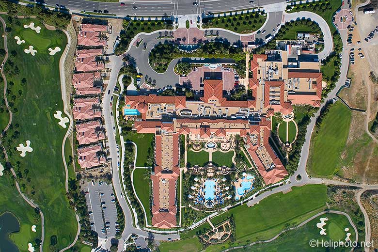
Essential Information

EXPERIENCE Over 20 years of aerial photography + video shoot experience has taught us what specific aerial views most likely suit your purposes. We foster longstanding relationships with a wide variety of clients and their recommendations are at the core of our success.

HELICOPTER-AIRPLANE-DRONE The altitudes aerials need to be shot at dictate the aircraft. Very low level close-ups can be shot with drones but legal limitations apply; please visit our drone regulations page for clarification. For real estate purposes we prefer to shoot from helicopters, as we can get low level close-ups and higher-up angles that show commercial centers or freeways in the vicinity. Such relationships can only be seen from about 800 ft. and higher.

PRICING Our rates are very competitive. For info please call us at 310 455-2821, we would love to talk to you in person. Or e-mail us with specifics and we will send you an estimate.

TIMING Usually we need a few days notice to schedule a shoot, the more notice we get the more we can take the weather into consideration.  Allow for 1-3 days turn-around time for pdf proof sheets or web gallery proofs. Rush jobs can be done on short notice and delivered within hours. All shoots are executed when weather and safety permit.

CAMERA EQUIPMENT We shoot aerials with the newest high-end Canon cameras and use a wide variety of lenses. Our aerial videos are shot in 1080HD or 4k, for details please visit the video page.

PROOFS, IMAGE FILES & PRINTING Proofs are shown via pdf proof sheets or web photo galleries, so our clients can view their images asap after the shoot. All final images leaving our office are custom corrected. To read about our digital imaging /editing processes please visit that page. We deliver our larger photo files via ftp uploads. Enlargements up to 42″ wide are printed in-house on our high-end Epson photographic printer.

Please visit our portfolio or client list pages to view the variety of clients and projects we have served.

Altitude: 500ft

Altitude: 1000ft

Altitude: 2000ft

Altitude: 3000ft

• Aerial Index
• Assignments
• Research Form

Learn How to Use Best Drones for Aerial Photography

Photography, especially aerial photography, has an exciting new aspect - Drone Photography. Using drones to capture stunning aerial photography images is not only much more straightforward and accessible now, but it's also lots of fun. With the costs of getting equipment for drone photography dropping fast, professionals and hobbyists are increasingly using drones for aerial photography.

What is Aerial Photography?

When you take pictures from any flying object, it is aerial photography. These flying objects can be a drone or even a kite. Other mediums which can be used are balloons, pigeons, helicopters, unmanned flying vehicles, fixed wing, etc.

Let's get started with how you can master the art of aerial photography using drones:

Finding the right equipment:.

There is a vast range of drones (also known as quadcopters or UAVs - unmanned aerial vehicles) available now on the market. Consider these two factors when choosing the right drone for your aerial photography:

• The flying capabilities of the drone.
• The camera that the drone can support

How much does a drone cost?

As with all of the modern technology, there are a lot of options available, and it mostly boils down to how much you are willing to invest. The advanced drone models that come with lots of controls and are powerful enough to lift your DSLR costs anywhere near $6500 and upwards.

However, for most purposes, even including professional aerial photography, you would not have to spend that much. You can find good quality drones fitted with cameras under $1500. Some drone models also support attaching a GoPro camera.

In this money, you will be able to get a drone with 15-20 minutes of flight time and also have inbuilt technologies such as collision avoidance and return-to-home feature wherein a drone can automatically return to home if the battery is running low or if you lost sight of the drone. Typically, the inbuilt cameras will have the ability to shoot 4K videos and take drone photo of up to 16 MP.

You need to do a lot of research when selecting the drone you want to buy. The Phantom range of drones by DJI is the first choice for many, and the Phantom 3 series model is one of the top-selling drones and is very popular for aerial photography.

Most drones these days are quite easy to operate and can pretty much "fly straight out of the box." The learning curve is minimal - get the drone's battery charged, install the controller app on your mobile device, sync your domain with your mobile app, and start flying. You can control the drone easily with their joystick type controllers that use your mobile device as a viewfinder. It's almost like playing a video game, only its real and much more fun.

Getting started with aerial photography

While there are easy to fly drones available in the market, it does take some getting used to, to start getting good shots. Start slow in a vast open space - a park or even the countryside. Making sense of and getting your bearings on what your camera is seeing through the smartphone app can get a little getting used to. You can set limitations in your mobile app regarding how high or far the drone can fly and always keep the drone in the line of your sight. Experiment with angles and zooms and click away. You would have to review your results and experiment to develop your skills to achieve the best aerial photography results with drones.

Follow the rules and regulations of your area

Most cities, states and even countries have now drafted rules that govern how you can use your drone, the height to which you can fly and what you can / or cannot click from the sky. In the US, the FAA has laid out the rules for flying drones; You can check out the rules here.

However, many of these rules only apply if you are flying drones for commercial purposes (if you are doing an aerial photography assignment and getting paid for it, the rules will apply).

However, for the recreational use of drones, the rules are much simpler. You don’t need a permit, and there are no pilot requirements for recreational use of drones. You do however have to register with the FAA. Visit this page and register your drone with the FAA before you start flying. It's a pretty simple process and costs just $5.

• Make sure that you study the rules and check-up with local authorities before you start. Usually, the rules are along these lines:
• Make sure you can always see your drone which means that you should fly the drone to be in your Line of Sight (LOS)
• Typically the maximum permissible height is around 400 feet.
• Respect the privacy of other people. Do not click images of private properties.
• Do not fly your drones overcrowded areas.
• Do not fly your drone near airports or any other no-fly zones specified by the authorities.

Getting better at Aerial Photography

Mastering drone photography is a unique aspect that you can add your photography. Shooting from 400 feet up in the sky creates stunning and intriguing images that show our world from an entirely different perspective.

As you start exploring aerial photography, you will find that it follows the same principals of other forms of photography – getting the light right, finding that unique frame and creating visuals that are expressive and tell a story.

Here are some tips you can follow to get better at aerial photography:

Learn how to work with the limitations of your drone camera.

Drone cameras are typically designed for shooting great videos, and most of them can shoot 4K videos. However, when it comes to taking still shots, they are no match to the DSLRs that you are using as a photographer.

Most drone cameras have tiny sensors just like compact cameras or camera on most high-end phones these days. These make their dynamic range limited, and low light performance is not excellent. The resolution is also typically not more than 16-20 MP.

Also, most drone cameras have wide-angle lenses with a fixed focal length. While all of this may sound limiting, in theory, you can take surprisingly good aerial photographs within these limitations. You wouldn't need low light performance as you would only shoot in the daytime (rules restrict the use of drones only in daylight) and since you are shooting from afar, depth of field isn't going to be a problem. Drone cameras are getting better and better by the day.

Fly low to take the best pictures

While your drone can fly as high as 400 ft, to make the best shots fly at a much lower height of 100-150 ft. Flying lower will give an interesting perspective and also establish a clear horizon for your images. If you want to take perfect top shots, then you do need to go as high as you can to cover the most area.

Start by shooting in automatic mode

As a professional photographer, you would mostly be shooting in manual mode with full control over all the factors. However, with a drone-mounted camera, it's better to shoot in automatic mode and to rely on camera's inbuilt auto-mode functions as the view mode you get in your mobile phone app is not an accurate picture of what the shot will be like. As you get more conversant with how the camera performs under various conditions, you can start using the manual mode as well.

Use bracketing

Most drone cameras support 3-step bracketing. This is a great feature that you can use to get three options for every shot you take (an underexposed and overexposed variation along with the standard image). You can choose the best image later and can also blend exposures using post-processing software.

Use filters

Since most drone cameras have only one aperture setting, you have limited controls over shutter speeds as well. You can control this somewhat by using neutral density filters that reduce the amount of light that gets into the camera lens, hence making the camera slower shutter speed. You can also use polarising filters to cut out the reflections or the harshness of the sun rays and get deeper, more vibrant blue skies.

Avoid your drone’s blades appearing in your pictures

Make sure you keep your drone's blades out of your picture frame. If you are careful, you can end up with your drones blades intruding in your photo frames. To avoid drone blades, keep your drone camera tilted slightly downwards.

Commercial Applications for Drone Photography

Be it a wedding photographer, a landscape photographer, or any other commercial photographer, drones add more value to your drone photography business and can increase your pay manifold. But before you enter the business side, find out what the drone photography rates are in their market based on the skill level, and set your prices accordingly. While creating stunning images of earth from the sky is it's own high and can be pursued purely as a creative art, here are some of the other exciting applications where you can become a professional drone photographer:

1. Real Estate Drone Photography

Using drones to undertake real estate photography can make you stand out from the crowd. Real estate drone photography is flourishing as the images captured through drones add a unique perspective to the real estate property being sold. Aerial real estate photography imparts a more clear understanding of the property and its neighborhood and increases the chances of the property getting sold quickly, manifold.  

2. Sports / Motion Photography

It won't be long before drones would be used full-fledged in sports photography  and motion photography after already making a great show at the Sochi Olympics. Drones in sports photography mean not only accessible pictures of aerial sports like ski and snowboarding but also a distant and clear view of all sports. Now, there isn't a need to fix multiple cameras on different location during a racing/sports event. A remotely operated drone can capture the moves of the sportsman at different periods. A great example would be Airdog. It has created the auto-follow action sports quadcopter for this very purpose.

3. Filmmaking

Given the relatively low cost of drones (much cheaper than the costs of hiring a helicopter or airplane), drones are already changing the face of cinematography. The idea of drones is opening alternative avenues to crane/helicopter shots. Many filmmakers are excited about the future of drone technology, which would enable better cinematography. Read our article to understand what is cinematography and how to devise a visual language to tell your own unique story.

4. Aquatic photography

How does the seabed look? How could one capture the moments spent underwater with family? Ziphius, the aquatic drone has answered many questions. Ziphius is the first smartphone-controlled aquatic drone which comes with multifarious utility. And guess what? It not only enables you to click pictures and videos but also plays with you!

5. Studio lighting for photoshoots

Lighting up a photoshoot involves an array of tasks such as setting up reflector discs, flashlights, convertible photo umbrellas, and a lot of power cables. It can not only be cumbersome but also limiting because of the fixed position of the lights. The researchers at MIT recently discovered the portable and automated alternative to drones. A drone equipped with light could be used by the photographers and shifted according to light needs, merely with a remote. The invention has proven to be a boon to the photographer fraternity and ensured boundless creativity.

6. Wedding photography

Clients who are ready to pay premium prices, opt for drone photography services at their wedding. Drone wedding photography gives them a different perspective they are looking for. With new regulations coming out for using drones in wedding , the drone industry is on rapid growth. The new drones coming out in the market are well equipped to be managed in a limited space, and photographers are making use of that.

Conclusion:

Drones are revolutionizing the very face of aerial photography services in every way. Though issues of legality and privacy plague the advent of drones, it'll be interesting to discover what new use-cases of the drones the future lays bare. So, expect to see lots of amazing images shot from the sky as photographers experiment more-and-more with techniques and grow their aerial photography business.

Do share your experiences about drones for aerial photography in the comments. Don't forget to add links to the images that you have shot from the sky!

Create your photography portfolio website on Pixpa in minutes. No coding required. Get started for free.

Try Pixpa - the easy, all-in-one portfolio website builder loved by photographers & creators.

Explore More Articles See all articles

Top-rated by creatives for 10+ years

All-in-one website builder for creatives.

Build Your Website

Start an Online Store

Sell Images

Marketing Tools

Client Galleries

Photo Gallery Apps

Start a Blog

Creatives love Pixpa

15-day free trial. No credit card required.

Beautiful Templates Made for Creatives Awesome Support Really Easy to Use Affordable Pricing

Rated as top website builder by creatives for 10+ years.

What's new on Pixpa

Recently Updated

• Mexican American Border Aerial Photographs
• Imperial County California Aerial Photography
• Mexico Aerial Photographs
• Arizona Aerial Photographs
• Agriculture and Farming Aerial Photographs
• Highways and Freeways | Aerial Photographs
• Irrigation | Aerial Photographs
• Lake County California | Aerial Photography
• Napa County California Aerial Photography
• Solar Farms Panels and Arrays | Aerial Photography

Aerial Index (Quick Links By Location and Subject)

Aerial Archives maintains an extensive collection of aerial photography, aerial photo maps and satellite imagery.

To search the collection of aerial photography and satellite imagery use the search box located at the top right of each page.   More advanced search options are recommended if you need an aerial photograph created after a specific date, containing more than one word or with a certain orientation (landscape, portrait).  Please select "Search" from the menu above for the advanced search options.

Aerial Archives creates aerial photography on assignment and provides historical aerial photography and research services.

Thank you for visiting nature.com. You are using a browser version with limited support for CSS. To obtain the best experience, we recommend you use a more up to date browser (or turn off compatibility mode in Internet Explorer). In the meantime, to ensure continued support, we are displaying the site without styles and JavaScript.

• View all journals
• My Account Login
• Explore content
• About the journal
• Publish with us
• Sign up for alerts
• Open access
• Published: 25 May 2024

Early aerial expedition photos reveal 85 years of glacier growth and stability in East Antarctica

• Mads Dømgaard   ORCID: orcid.org/0000-0001-5066-7514 1 ,
• Anders Schomacker   ORCID: orcid.org/0000-0002-8031-9008 2 ,
• Elisabeth Isaksson 3 ,
• Romain Millan   ORCID: orcid.org/0000-0002-7987-1305 4 ,
• Flora Huiban   ORCID: orcid.org/0000-0002-3582-1840 1 ,
• Amaury Dehecq 4 ,
• Amanda Fleischer 1 ,
• Geir Moholdt   ORCID: orcid.org/0000-0002-8883-1620 3 ,
• Jonas K. Andersen 1 &
• Anders A. Bjørk   ORCID: orcid.org/0000-0002-4919-792X 1  

Nature Communications volume  15 , Article number:  4466 ( 2024 ) Cite this article

4367 Accesses

295 Altmetric

Metrics details

• Climate-change impacts
• Cryospheric science

During the last few decades, several sectors in Antarctica have transitioned from glacial mass balance equilibrium to mass loss. In order to determine if recent trends exceed the scale of natural variability, long-term observations are vital. Here we explore the earliest, large-scale, aerial image archive of Antarctica to provide a unique record of 21 outlet glaciers along the coastline of East Antarctica since the 1930s. In Lützow-Holm Bay, our results reveal constant ice surface elevations since the 1930s, and indications of a weakening of local land-fast sea-ice conditions. Along the coastline of Kemp and Mac Robertson, and Ingrid Christensen Coast, we observe a long-term moderate thickening of the glaciers since 1937 and 1960 with periodic thinning and decadal variability. In all regions, the long-term changes in ice thickness correspond with the trends in snowfall since 1940. Our results demonstrate that the stability and growth in ice elevations observed in terrestrial basins over the past few decades are part of a trend spanning at least a century, and highlight the importance of understanding long-term changes when interpreting current dynamics.

Similar content being viewed by others

Historical glacier change on Svalbard predicts doubling of mass loss by 2100

Accelerated global glacier mass loss in the early twenty-first century

Two decades of glacier mass loss along the Andes

Introduction.

The East Antarctic Ice Sheet (EAIS) contains more than 52 m of potential sea level equivalent (SLE) 1 . Recent observations indicate that the EAIS is more vulnerable than previously anticipated 2 , and has made a considerable contribution to the continent-wide mass loss during the past decades 3 . The losses have primarily occurred in some of the marine-based catchments in Wilkes Land 4 , and are largely attributed to the intrusion of modified Circumpolar Deep Water (CDW) 2 . The terrestrial catchments, where the majority of the ice is grounded above sea level, have recently shown a mass gain caused by increased accumulation 5 , 6 , 7 , 8 , which has balanced some of the overall mass loss 9 , 10 . Observational time series of glaciers in East Antarctica pre-dating the satellite era are rare 11 and consequently not long enough to determine if recent trends are independent of natural fluctuations 2 , 12 . Historical datasets from early expeditions serves as a crucial link connecting records from the pre-satellite era, such as those derived from ice cores 13 or geological 14 and geomorphological evidence 15 , to quantitative observations of mass change acquired from satellites 5 , 6 , 7 . While geological and geomorphological records cover longer time scales with temporal uncertainties of up to thousands of years 14 , 15 , SMB estimates from ice cores are generally very local and spatially confined 16 . In contrast, data from historical aerial expeditions often provide extensive coverage across large areas, with detailed temporal and spatial information 17 , 18 , 19 . Additionally, historical data provide an important baseline for forward modeling of glacier dynamics, allowing for long-term reanalysis data and more accurate model calibration 20 . In Greenland and Svalbard, long-term observations from historical aerial images have been vital for determining the historical response of glaciers to climate change 18 , 19 , 21 , 22 . However, in Antarctica, the scarcity of historical climate data makes climate reanalysis estimates before the 1970s largely uncertain 10 , 23 , and observed trends cannot clearly be distinguished from natural variability 24 , 25 .

Here, we rediscover and utilize the images from the earliest large-scale aerial photography campaign conducted on the Antarctic continent, allowing us to extend the era of observational records of glacier evolution back to the 1930s. Since the beginning of the 20 th century, several expeditions were launched to Antarctica with the aim of exploring and capturing aerial images for the production of geographical maps 26 , 27 , 28 , 29 , 30 . However, just a handful of studies have previously used these data for generating digital elevation models (DEMs) and only for glaciers located in West Antarctica and the Antarctic Peninsula 11 , 31 , 32 , dating back to 1947 32 . On the Antarctic Peninsula, these observations show widespread near-frontal surface lowering and inland stability since 1960 31 . On the other hand, historical observations of the Byrd Glacier over the past 40 years indicate a constant surface elevation, stable grounding line, and surface flow velocity 11 .

Here, we study 21 glaciers located in three regions along c. 2000 km of the EAIS, from Lützow-Holm Bay (38° East) to Ingrid Christensen Coast (79° East) (Fig.  1A ). All glaciers are marine-terminating outlets of the EAIS, varying in width from 2 to 10 km, and with the fastest flow speeds reaching 2 km/yr. Some have large floating ice tongues, while others have their frontal position close to the grounding line. The glaciers are located in basins containing around 2.6 M km 3 of ice (SLE 7.23 m), and the specific sub-regions studied (Fig.  1A ) contain 0.42 M km 3 of ice (SLE 1.15 m) 1 . In recent decades, these regions have maintained balance or gained mass 3 , leading to advances in terminus 33 and grounding line position 34 , 35 , during a period of substantial mass loss and terminus retreats occurring at other sectors of the Antarctic Ice Sheet 3 , 5 , 6 , 7 , 33 , 34 , 36 , 37 , 38 , 39 .

A Existing historical glacier reconstructions (Byrd 11 , Moider 32 and Peninsula 31 ) and glaciers included in this study (frontal reconstructions n  = 21, elevation reconstructions n  = 12, velocity reconstructions n  = 4), overlaid on 2003–2021 Antarctic annual elevation change from Smith et al 5 ., with MEaSUREs basin 72 . B Taylor glacier in 1937, 1956, and 1973 as captured in the aerial images. Close up shows the different types of fiducial marks used for standardizing the internal image geometry. C Produced digital elevation models (DEM) overlain on orthomosaics generated from interpolated DEMs. For the productions of the 1956 DEM and orthomosaic we included additional oblique images (not included here) as the glacier was photographed with a trimetrogon camera setup.

In late 1936, the Norwegian whaling entrepreneur Lars Christensen initiated his fifth and final expedition (Thorshavn IV) to Antarctica with the specific aim of capturing aerial images for producing the earliest detailed maps of the East Antarctic coastline. Drawing inspiration by the Greenland aerial expeditions in 1932 40 and the aerial mapping of Svalbard in 1936 19 , the coastline was photographed with an oblique angle and a stereo overlap of c. 60%. The expedition acquired 2200 photographs covering approx. 2000 km of the coastline from 82° to 20° East 30 (Fig.  1A and Supplementary). Twelve topographic maps of the coastline were produced from the images. However, they were not published until 1946 due to the German occupation of Norway. Since then, the images have been stored at the Norwegian Polar Institute in Tromsø and largely forgotten 41 , 42 . Luckily, the film has been kept at optimal conditions, giving us the best possible starting point for recreating the historical East Antarctic glacier conditions with modern digital technologies.

The images from the Norwegian 1936-37 expedition are unique, as they provide the earliest detailed view of a regional Antarctic coastline and allow historical reconstruction of glaciers in East Antarctica. The image archive poses considerable challenges for analysis due to its limited camera metadata, sparse flight line and camera position information. Consequently, a comprehensive manual image selection and geolocation process is essential prior to conducting any analysis (Methods). Moreover, the vast majority of the images are captured from low elevations or large distances from the coast, have poor image contrast and/or are overexposed. Additionally, the majority of East Antarctic coastline lacks visible bedrock features, which are essential for producing reliable results (Methods). Nevertheless, we have successfully identified 128 images, with sufficient overlap, contrast and bedrock presence for ground control. The Norwegian 1936/37 imagery is combined with more recent historical aerial photographs (1956–1973) from Australian aerial campaigns (Fig.  1 ) and also with modern satellite data. This allows us to quantify changes on a decadal timescale throughout the 20th and 21st Century.

We utilize a total of approximately 300 aerial images to examine changes in glacier elevations, velocities, and terminus positions (Methods). We reconstruct past ice sheet configurations by processing the historical aerial images using structure-from-motion (SfM) photogrammetric techniques 43 , 44 , to provide the, to date, most extensive historical assessment of regional glacier dynamics in Antarctica. The SfM models are georeferenced to real-world coordinates by GCPs across the study area and transferring the coordinates from modern high-resolution stereo satellite imagery 45 . The uncertainty of our historical reconstructions is determined by comparing the historical surface to a modern reference surface over stable bedrock (Methods).

From the aerial imagery we are able to quantify elevation changes of 12 glaciers (Methods). The produced DEMs vary in pixel size from 8 m to 25 m, and the elevation uncertainty ranges from 1.6 m to 9.9 m depending on the imagery and location (Methods). Based on the historical DEMs, we perform orthorectification of the aerial images and generate orthophoto mosaics with a pixel size ranging from 1 to 8 m. Due to the extensive collection of aerial images captured in the 1950s, we are able to measure the historical flow speeds of four glaciers, where the image reacquisition interval successfully matches glacier flow speeds. Lastly, we determine frontal changes of 21 glaciers from 1937 to 2023 (Table  S1 and Fig.  S11 ). From the 85 years of observations, we find two distinct regional patterns; one of constant glacier surface elevations and one of ice thickening.

Historical frontal retreat and constant long-term ice elevations in Lützow-Holm Bay

Despite large variations in size and characteristics, all six glaciers in Lützow-Holm Bay experienced a net retreat between 1937 and the 1980s, when they reached an almost simultaneous minimum (Fig.  2 ) associated with a complete break-up of fast ice in the bay 35 , 46 . Another smaller retreat phase occurred around the mid-2000s, with the exception of Shirase, and again during 2016-18 47 . By far, the largest fluctuations are observed at Shirase Glacier with a total range of almost 90 km in the ice-front position from its 1963 maximum to its minimum in 1988. In contrast, Langhovde and Hovdebreen Glacier show frontal variations of less than 1 km between 1937 and 2023. Since the retreat in the 1980s, all glaciers except Langhovde and Honnörbrygga have, at some point, advanced to a similar marginal position or even extended beyond their extent recorded in 1937. The frontal collapse of Honnörbrygga Glacier from 1937 to 1956 was observed in 1964 42 , but has never before been quantified. From 1956 to 1974, Honnörbrygga Glacier retreated an additional 4.5 km, resulting in a total retreat of more than 10 km. Since 1974, the glacier has been able to regrow less than half of its total retreat. From its current position, it would require 17 years of uninterrupted advance at its current flow speed in order to reach its 1937 maximum extent.

A Lützow-Holm Bay, ( B ) Kemp & Mac Robertson Land, and ( C ) Ingrid Christensen Coast. The changes in frontal position is shown relative to the glacier-specific maximum. Forbes Glacier is shown with two frontal positions, as it has two separate floating extensions. Changes in elevation are shown as the annual rate of change in m/yr between successive observational periods, with the shaded area indicating the model uncertainty (1σ) of the produced digital elevation models (DEM) (Methods). The hatched areas represent the sampling uncertainty (2σ + 1.5 m) associated with the sensitivity of the calculated changes (Supplementary). Note that the y-axis values for frontal positions differ among glaciers.

The retreat of Honnörbrygga Glacier has not led to a thinning of its grounded section between 1937 and 2020. The mean surface elevation change rate during this period is insignificant at +0.01 m/yr ± 0.10 m/yr from 1937 to 2016 and +0.24 m/yr ± 1.08 m from 2016 to 2020. A similar pattern of unchanged elevations is evident all along the Syowa Coast from 1937 to 2016 (Fig.  S12A ), with rates of +0.01 m/yr ± 0.10 m/yr and +0.03 m/yr ± 0.10 m/yr at Langhovde and Hovdebreen Glacier, respectively (Fig.  2 ). Between 2016 and 2020, DEM differences indicate a slight negative rate of change, −0.43 m/yr ± 0.74 m/yr for Langhovde and −0.25 m/yr ± 0.74 m for Hovdebreen. Consequently, the absolute elevations have remained unchanged throughout the entire observation period from 1937 to 2020 (Fig.  S23 ). Modern altimetry-based observations covering the years 2003 to 2021 5 confirm limited surface elevation changes along the Syowa Coast, with rates ranging from +0.02 m/yr ± 0.01 m/yr to +0.06 m/yr ± 0.05 m/yr, except for Shirase Glacier, which exhibited thickening at a rate of +0.53 m/yr ± 0.27 m/yr.

Regional frontal fluctuations and long-term ice thickening

Our observations show no regional long-term trend in the frontal positions of the studied glaciers in Kemp Land, Mac Robertson Land, and along Ingrid Christensen Coast between 1937 and 2022. The glaciers fluctuate between periods of frontal advances and retreats of varying distances (<0.1 km to 13.5 km) and intervals (3–50 years). Most noticeable is the 13.5 km advance of Mulebreen Glacier since the 1980s and the retreat of Jelbart Glacier, which is 3.5 km short of its 1937 marginal position.

From the historical DEMs, we observe an overall thickening of the glaciers in Kemp and Mac Robertson Land between 1937 and 2021 and along Ingrid Christensen Coast between 1960 and 2021 (Fig.  2 , Fig.  S23 ). In Kemp and Mac Robertson Land, the largest changes are observed at Hoseason and Taylor Glacier, with an annual average surface elevation increase of +0.23 m/yr ± 0.07 m/yr and of +0.11 m/yr ± 0.05 m/yr since 1937, respectively. In comparison, Utstikkar, Jelbart, and Brunvoll Glacier show less thickening since 1937, with rates of +0.06 m/yr ± 0.04 m/yr, +0.04 m/yr ± 0.04 m/yr, and +0.04 m/yr ± 0.22 m/yr, respectively (Fig.  S23 ). For Jelbart and Utstikkar Glacier, the thickening is substantially larger ( + 0.11-0.14 m/yr ± 0.04 m/yr since 1937 and +0.13-0.42 m/yr ± 0.04 since 1973) when excluding observations from the hummocky dynamic frontal regions where surface undulations result in short-term dH variations of up to ±20 m. (Fig.  S15 ).

Along Ingrid Christensen Coast, the largest thickening is observed at Shennong Glacier with an average rate of +0.17 m/yr ± 0.06 m/yr from 1960 to 2011 (Fig.  2 ). At Flatnes, Hovde, and Brown Glacier, the rates are smaller, ranging from +0.06 m/yr ± 0.02 m/yr to +0.11 m/yr ± 0.05 m/yr (Fig.  2 ). Between 2011 and 2021, DEM differences show negative rates for Hovde and Flatnes Glacier (−0.23 m/yr ± 0.15 m/yr and −0.07 m/yr ± 0.15 m/yr), positive rates for Shennong (+0.26 m/yr ± 0.15 m/yr), and rate close to zero at Brown Glacier. In total, all glacier along Ingrid Christensen Coast experienced an absolute elevation increase from 1960 to 2021/2022 (Fig.  S23 ). Despite the long-term thickening of the glaciers in Kemp and Mac Robertson Land and along Ingrid Christensen Coast, our results reveal variations in the magnitude of the rates and periods of thinning. Specifically, Taylor and Utstikkar Glacier experienced thinning between 1956/1960 and 1973, Jelbart from 1937 to 1973, and Hoseason, Flatnes, and Hovde exhibited thinning during the past decade (Fig.  2 ). These findings suggest low magnitude decadal variability superimposed on a pattern of long-term thickening.

Our analysis of historical velocities of glaciers in Kemp and Mac Robertson Land reveal a pattern of constant flow velocities since the 1950s (Fig.  3 ). The historical velocities have an uncertainty range of 7.2 m/yr to 10 m/yr, and for Taylor, Jelbart, Hoseason and Utstikkar Glacier, the historical velocities fall within the range of modern satellite-derived velocities from 2006-2018, even when disregarding the 2006-2013 annual velocities with a high level of uncertainty.

The shaded area shows the uncertainty in historical velocity estimates, defined as the combined the uncertainties of the mean square positional error (MSPE) and the manual error associated with feature positioning (Methods). Historical velocities are estimated by manually tracking the movement of crevasses between sets of orthophoto mosaics. Modern velocities and associated uncertainties are extracted from the ITS_LIVE annual velocity mosaics 67 (Methods).

The absence of pronounced regional trends in frontal position in Kemp and Mac Robertson Land and along Ingrid Christensen Coast is in line with existing observations of basin-wide median frontal movement rates between 1974 and 2012 33 . Historical observations of glacier terminus positions from other regions in East Antarctica reveal cyclic behavior with no overall trend from the 1950s to the late 1990s 48 . Contrary, on the Antarctic Peninsula, the majority of glaciers have retreated since the 1950s with a suggested link to atmospheric warming 39 . In Wilkes Land, East Antarctica, a recent anomalous frontal retreat has been linked to a reduction in sea ice 33 . Additionally, land-fast sea ice played an important role in the observed simultaneous frontal retreat of the glaciers in Lützow-Holm Bay in the 1980s 35 , 46 and again from 2016 to 2018 46 , 47 . Moreover, the 2016-2018 retreat was coupled to a decrease in surface elevation and an acceleration in flow at Shirase, Skallen, and Telen Glacier, whereas Honnörbrygga and Langhovde Glacier were unaffected 47 . Similarly, our findings of a long-term frontal retreat at Honnorbrygga and Langhovde Glacier since 1937 does not coincide with any changes in the surface elevation of these glaciers (Fig.  2 ), suggesting that these floating ice tongues have provided limited buttressing on a decadal time-scale. Additionally, our results indicate that the land-fast sea-ice conditions controlling the frontal position of Langhovde and Honnörbrygga Glacier have become more susceptible to break up during the past 85 years. Notably, recent findings have pointed towards a possible link between these localized sea-ice breakups and the detection of Warm Deep Water (WDW) beneath Langhovde Glacier in 2018 49 .

The terrestrial regions of the EAIS respond mainly to atmospheric forcing 2 . Overall, there has been no significant trends in annual or seasonal mean air temperature in East Antarctica since the 1950s 50 , and mean austral summer air temperature (December to February) from stations in all regions rarely exceeds 0 °C (Fig.  4C ). This suggests that surface melting have played a minimal role in the documented ice thickness changes overtime. However, at Davis station we do observe periods of above zero-degree temperatures during the 1970s and 2000s, which have caused intervals of increased ablation in this region near sea level.

A Glacier elevation changes are calculated as the mean elevation change (dH) over the longest period for each region. B ERA5 mean annual snowfall in mm water equivalent (w.e.) from 1940 to 2022 for each region (Fig.  S21A ), plotted as 5-year running average. Linear trend is calculated based on the running average since 1940 (dashed line) and 1979 (dotted line). Rate of change is given for the period 1940–2022 in mm per decade. C Mean summer air temperature (December, January, and February) from station measurements (dotted line) and ERA5 2 m temperature data, plotted as 5-year running average.

While previous research on Antarctic snowfall found no statistically significant changes since the 1950s 51 , recent studies utilizing compiled data on ice core records indicate increased Antarctic-wide snow accumulation during the past 200 years 10 , with links to atmospheric warming 52 , ozone depletion 53 , and a positive shift in Southern Annular Mode (SAM) 10 . Nevertheless, there are notable regional differences in accumulation in both sign and magnitude, and in East Antarctica the results are derived from only a few ice core records 10 .

ERA5 reanalysis data suggest a consistent positive long-term trend in mean annual snowfall along the coastline of Kemp and Mac Robertson Land, and Ingrid Christensen Coast since the 1940s, whereas in Lützow-Holm Bay, snowfall has remained almost constant (Fig.  4B ). The long-term trend is most pronounced in Kemp and Mac Robertson Land, where snowfall increased by ~50 % between 1940 and 2022, corresponding to 17.3 mm of water equivalent (w.e.) per decade, whereas along Ingrid Christensen Coast, the increase is around 15% equivalent to 5.3 mm w.e. per decade. Thus the trend in snowfall corresponds with the observed long-term historical changes in glacier elevations in each of the respective regions (Fig.  4 ). Observation-based atmospheric reanalysis data of Antarctica are questionable prior to the satellite era due to a lack of historical data 23 , particularly concerning snowfall 10 , 51 . The trend in snowfall since 1979 is nearly identical trends to that from 1940 for all regions (Fig.  4 ). However, to differentiate the increase in snowfall from long-term background noise, larger trends or longer-time series are needed 25 . Nevertheless, we hypothesize that the observed increase in surface elevation since 1937 in Kemp and Mac Robertson Land (Fig.  4 ) is likely a result of changes in precipitation patterns. The absence of dynamic ice changes, observed from stable frontal positions since the 1930s and flow velocities since the 1950s (Figs.  2 ,  3 ) suggest that the observed ice surface increase results from the increase in precipitation (Fig.  4 ). The periodic thinning and decadal variability observed within the long-term trends in glacier surface elevation in all regions (Fig.  2 ), demonstrates the natural variability inherent in these systems. Moreover, it highlights the importance of long-term glacier records, as studying these short-term changes without the long-term perspective could lead to erroneous conclusions.

Basin-wide altimetry-derived elevation changes of each of the studied sub-regions show an overall increase in elevation between 1985 and 2022 7 (Fig.  S22 ). This trend is consistent with the observed historical glacier thickening in Kemp and Mac Robertson Land and along Ingrid Christensen Coast. Contrary, in the Prince Olav Coast sub-region, which includes the Lützow-Holm Bay area, the basin-wide trend deviates from the observed long-term constant ice elevations. This suggests that the basin-wide increase is not significant on a long-term scale, or more likely, that the constant ice elevations in Lützow-Holm Bay are largely confined to this region. Other parts of Dronning Maud Land have experienced a substantial mass gain in the past two decades caused, in part, by anomalously high snowfall in 2009 and 2011 5 , 6 , 8 . Additionally, the recent mass gain of the Shirase Glacier (Fig.  2 ) has been linked to strengthening easterly winds reducing the inflow of modified Circumpolar Deep Water and decreasing basal melt rates 35 .

Our historical observations of ice-thickness changes provide valuable insights into historical mass balance estimates of East Antarctica, as in situ records of mass balance are extremely few in Antarctica. Currently, the earliest ice-sheet wide mass balance estimates start in the late 1970s 3 , 6 , 7 , and since then all the sub-regions examined in this study have exhibited either an overall mass gain or been relative unchanged. Given that our historical reconstructions extends beyond the era of reliable climate reconstruction, and considering the limited magnitude of the observed long-term changes and their localized spatial resolution, we are unable to further deduct the specific drivers of the observed changes. Regardless of potential climatic changes, our results indicate that the glacier in Kemp and Mac Robertson Land and along Ingrid Christensen Coast, have accumulated mass during the past 85 years which inevitably have mitigated parts of the more recent mass loss from the marine basins in East Antarctica and the West Antarctic Ice Sheet (WAIS). This positive accumulation trend and positive mass balance is anticipated to persist as snowfall is expected to increase over the entire EAIS in the next century 54 , 55 , and ice sheet modeling studies project positive mass balance estimates in all three sub-regions across all future RCP scenarios 56 .

The 1936-37 aerial photographs

The original negatives from the 1936-37 Thorshavn IV expedition were digitized using a photogrammetric scanner at a resolution of 0.014 mm. Aerial photographs captured with a similar camera type have successfully been used for reconstructions of local and large-scale terrain models in Svalbard 19 , 57 . However, the Antarctic imagery contains limited camera calibration information and none or very rough camera positions. Consequently, before initiating the image processing phase, we carefully examined each image from the expedition and manually tried to determine the geolocation of where along the coastline the image was captured. However, due to the absence of discernible surface features such as bedrock, ice rises, or distinctive coastline features along large parts of the East Antarctic coastline, geolocation was not always possible. Additionally, a large quantity of images are (i) captured from low elevations or considerable distances from the coastline, or (ii) exhibit poor contrast or overexposure, which further challenged the process (Fig.  S28 ). Consequently, our selection process led us to identify 128 images (Table  1 ) from the archive that aligned with the quality standards required for historical reconstructions and frontal mapping.

The 1954–1973 Australian image campaigns

The Australian Antarctic Data Centre holds a vast collection of aerial photographs acquired since the 1950s covering the Australian Antarctic Territory. The first major period of Australian aerial photography acquisition, from 1954 to 1965, was carried out by the Australian National Antarctic Research Expedition (ANARE) using Auster and Beaver aircraft and a K17 trimetrogon camera. From 1960, the vertical K17 in the trimetrogon system was replaced with a Wild RC9. Descriptive studies were published more than 50 years ago using the trimetrogon imagery 41 , 58 , 59 . In the 1970s, the Division of National Mapping carried out extensive photographing of the areas around Prince Charles Mountains and Enderby Land using a Wild RC 9 camera from a Pilatus Porter aircraft. The archive consists of digitized negatives scanned using a photogrammetry-grade scanner, and all images contain sparse camera calibration information and imprecise camera locations.

Structure for motion (SfM) processing

The aerial images are processed in Agisoft Metashape v. 1.7.4 using a standard SfM workflow 19 , 44 . We primarily process photographs from each period and glacier separately. However, in cases where glaciers are located in close proximity (such as Langhovde, Hovdebreen and Honnörbrygga, as well as Jelbart and Utstikkar), we combine the images into a single model for each period.

As a first step, we standardize the internal geometry of each image set by detecting the image fiducials and determining their mean position. Agisoft Metashapes Detect Fiducial function automatically identifies the fiducial center pixels while at the same time masking out the image frame 60 . The images are automatically scaled and oriented to ensure alignment of the fiducials. We manually inspected all fiducial positions and corrected any misplaced ones. All fiducials from the ANARE archive were manually placed. Next, we align the images by extracting up to 50,000 key points per images at Medium accuracy setting, meaning that photos are downscaled by a factor of four. For some image sets, additional tie points are manually placed to ensure the correct alignment of the images. The tie points are distinctive surface features (e.g., crevasses) that could be detected in multiple images. The image alignment solves for the unknown camera parameters, including the focal length, while estimating relative camera locations and orientations 44 .

For absolute georeferencing of the 3D model, GCPs are extracted from the Reference Elevation Model of Antarctica (REMA) 45 , 61 and manually placed in the aerial images. The GCPs are distinct features of stable bedrock with specified (x,y,z) locations. When possible, we use the same GCPs for glaciers photographed multiple times. As the amount and distribution of stable bedrock for GCP selection varies greatly among all of our study sites, an ideal distribution is not always possible 11 , 44 . Following GCP placement, a full bundle adjustment is executed on the aligned block which refines the exterior and interior camera orientation parameters as well as the tie point coordinates 44 , 60 . We perform a dense multi-view stereo (MVS) reconstruction, with a High quality setting, meaning that dense cloud is generated at 1:2 of the original image resolution, due to processing time. The point filtering is set to Moderate to Aggressive setting for outlier removal 19 . The dense cloud is imported into CloudCompare (v. 2.12) for additional filtering, removing points outside of the local minimum and maximum as well as obvious erroneous elevations. The point clouds are gridded into DEMs with a spatial resolution ranging from 6 to 25 m, reflecting the ground sampling distance of the point cloud. Lastly, orthophoto mosaics are produced with a resolution of 2–10 m. The lowest resolution is found in products derived from the 1936/37 photographs. In cases where the image quality is poor or bedrock visibility is limited, we are only able to generate reliable orthophoto mosaics and not DEMs.

DEM post-processing

All produced DEMs are co-registered to the REMA reference DEM using the method developed by Nuth and Kääb 62 . Following co-registration, we assess the absolute model accuracy by calculating the Normalized Median Absolute Deviation (NMAD) of the elevation differences over stable bedrock 63 , 64 . The accuracy vary from 1.6 to 9.9 m, with the 1936/37 DEMs being the least accurate. From the residual elevation difference values we compute spatial variograms for each of our produced DEMs to assess the degree of spatial autocorrelation in the models 19 , 64 . Using the xDEM python package 65 , we sample empirical variograms and fit a double-range variogram model consisting of a short-range Gaussian model and a spherical model at long ranges. Finally, we propagated the pixelwise uncertainties to the estimation of the overall uncertainty of the mean elevation change of each glacier 19 , 64 .

Estimation of glacier elevation changes

Due to a combination of insufficient image overlap, oblique view-angle, and low-contrast snow areas, the DEMs contain areas of no data (e.g., Fig.  S12 – S19 ). To account for data gaps and enable comparison of ice elevations across multiple periods, we calculate elevation changes (dH) of the entire glacier area as well as within 150-m radius circles, all located within the minimum boundary area defined by the GCPs (Fig.  S12 – S19 ). These circles are manually positioned across the glacier area in locations with a high density of elevation observations in all periods and with an aim of capturing the overall characteristics of the glacier (Supplementary). As a result, the number of circles placed varies between the glaciers. All elevation changes are calculated relative to the REMA reference DEM strip, as differencing two historical DEMs with data gaps results in more areas with no data. We incorporate a conservative uncertainty estimate of 1 m for the REMA DEM 45 into our calculations. By comparing the historical DEMs to the reference strip, we can ensure a more comprehensive assessment of elevation changes across the study area. Subsequently, we calculate the elevation changes between each historical period as:

where period3 is the REMA reference DEM strip. Finally, to determine the mean elevation change for each glacier, we compute the average dH of all circles placed within the glacier area, rather than using a hypsometric-weighted average, as the sampled variance in glacier surface elevation is limited and without a significant correlation to the observed dH (Fig  S24 ). This approach allows us to extract valuable information from the sparse DEMs and assess changes in glacier elevation over time. Post-2010 elevation changes derived from DEMs are calculated by subtracting co-registered REMA DEM strips. We test the sensitivity of our results to the placement of the circles by calculating the mean dH with a subsample of the circles, as well as by slightly shifting the positions of the circles (Supplementary).

Additionally, we extract ICESat and ICESat-2 derived elevation changes between 2003 and 2021 from Smith et al. 5 . We determine the elevation change of each glacier as the mean of the pixels closest to the grounding line.

Frontal position

We manually digitize the historical glacier frontal positions (1937–1973) from the produced orthophoto mosaics as well as from a combination of georeferenced aerial images and historical maps. Frontal positions from 1974 to 2022 are mapped from Aster and Landsat satellite images (Fig.  S25 , S26 , and S27 ). In cases where a glacier is heavily fractured, we define the frontal position as the crevasse that decouples the inner section from the outer section of the floating extension. We measured the frontal changes along an approximate centerline and relative to the maximum position of the terminus 66 .

By manually tracking the movement of glacial surface features between sets of orthophoto mosaics, we estimate historical ice velocities for Hoseason, Taylor, Jelbart, and Utstikkar Glacier in the late 1950s. These features are distinct crevasses that are easily identifiable in both sets of orthophoto mosaics, and are mainly found at the frontal part of the glacier. The number of detected features varies between glaciers, ranging from 4 at Taylor Glacier to 13 at Utstikkar Glacier (Fig.  S20 ). For each glacier, we calculate the mean displacement of all sets of corresponding features and determine the yearly velocity using the time between image acquisitions, ranging from 4 months at Hoseason to 4 years at Taylor. The errors from the manual tracking are determined by combining the uncertainties of the mean square positional error (MSPE) and the manual error associated with feature positioning. The manual error is set to 1 pixel to account for the limitation of placing features at subpixel levels. The MSPE is based on the x- and y-errors of the estimated GCP locations for each of the orthophoto mosaics, as reported in Agisoft Metashape. For 2006-2018 we use ITS_LIVE annual velocity mosaics 67 , 68 and calculate the mean velocity and error of all pixels found within the glacier surface area used for the historical velocity estimates (Fig.  S20S ).

Climate data and surface mass balance (SMB)

For each region of interest (Fig.  S21A ), we calculate the mean austral summer temperature (December to February) and mean annual snowfall between 1940 and 2022 from 0.25° ERA5 data 69 , 70 . Additionally, we calculate the mean austral summer temperature based on observational records from Syowa, Mawson, and Davis Station from the Scientific Committee on Antarctic Research (SCAR) Met READER project. RACMO2.3p2 annual surface mass balance (SMB) estimates 71 are extracted from 1979 to 2022 using the same regions of interest as for the ERA5 data.

Data availability

The produced DEMs, orthophoto mosaics, ice front positions, surface flow velocity, and dH estimates are accessible via figshare ( https://doi.org/10.6084/m9.figshare.23552079.v1 ). The REMA DEM can be downloaded from https://www.pgc.umn.edu/data/rema/ . Monthly mean surface air temperature records from Syowa, Mawson, and Davis Station are available via https://legacy.bas.ac.uk/met/READER/ . In addition, mean monthly ERA5 data on 2-m air temperature and snowfall are available from https://cds.climate.copernicus.eu/cdsapp#!/dataset/reanalysis-era5-single-levels-monthly-means . RACMO data is available upon request to Michiel R. van den Broeke and Melchior van Wessem. The Norwegian and Australian aerial images are available upon request to The Norwegian Polar Institute and The Australian Antarctic Division, respectively, owing to their ownership of the image rights.

Code availability

Codes used to produce the figures of this paper are accessible at ( https://doi.org/10.6084/m9.figshare.23552079.v1 ).

Morlighem, M. et al. Deep glacial troughs and stabilizing ridges unveiled beneath the margins of the Antarctic ice sheet. Nat. Geosci. 13 , 132–137 (2020).

Article   ADS   CAS   Google Scholar  

Stokes, C. R. et al. Response of the East Antarctic Ice Sheet to past and future climate change. Nature 608 , 275–286 (2022).

Article   ADS   CAS   PubMed   Google Scholar  

Rignot, E. et al. Four decades of Antarctic Ice Sheet mass balance from 1979–2017. Proc. Natl Acad. Sci. USA 116 , 1095–1103 (2019).

Article   ADS   CAS   PubMed   PubMed Central   Google Scholar  

Velicogna, I. et al. Continuity of Ice Sheet Mass Loss in Greenland and Antarctica From the GRACE and GRACE Follow-On Missions. Geophys. Res. Lett. 47 , e2020GL087291 (2020).

Article   ADS   Google Scholar  

Smith, B. et al. Pervasive ice sheet mass loss reflects competing ocean and atmosphere processes. Science 368 , 1239–1242 (2020).

Schröder, L. et al. Four decades of Antarctic surface elevation changes from multi-mission satellite altimetry. Cryosphere 13 , 427–449 (2019).

Nilsson, J., Gardner, A. S. & Paolo, F. S. Elevation change of the Antarctic Ice Sheet: 1985 to 2020. Earth Syst. Sci. Data 14 , 3573–3598 (2022).

Boening, C., Lebsock, M., Landerer, F. & Stephens, G. Snowfall-driven mass change on the East Antarctic ice sheet. Geophys. Res. Lett. 39 (2012).

Davis, C. H., Li, Y., McConnell, J. R., Frey, M. M. & Hanna, E. Snowfall-driven growth in East Antarctic Ice Sheet mitigates recent sea-level rise. Science 308 , 1898–1901 (2005).

Medley, B. & Thomas, E. R. Increased snowfall over the Antarctic Ice Sheet mitigated twentieth-century sea-level rise. Nat. Clim. Change 9 , 34–39 (2019).

Child, S. F., Stearns, L. A., Girod, L. & Brecher, H. H. Structure-from-motion photogrammetry of antarctic historical aerial photographs in conjunction with ground control derived from satellite data. Remote Sens. 13 , 1–25 (2021).

Google Scholar  

Gwyther, D. E., O’Kane, T. J., Galton-Fenzi, B. K., Monselesan, D. P. & Greenbaum, J. S. Intrinsic processes drive variability in basal melting of the Totten Glacier Ice Shelf. Nat. Commun. 9 , 3141 (2018).

Article   ADS   PubMed   PubMed Central   Google Scholar  

Frezzotti, M., Scarchilli, C., Becagli, S., Proposito, M. & Urbini, S. A synthesis of the Antarctic surface mass balance during the last 800 yr. Cryosphere 7 , 303–319 (2013).

Jones, R. S. et al. Rapid Holocene thinning of an East Antarctic outlet glacier driven by marine ice sheet instability. Nat. Commun. 6 , 8910 (2015).

Kawamata, M. et al. Abrupt Holocene ice-sheet thinning along the southern Soya Coast, Lützow-Holm Bay, East Antarctica, revealed by glacial geomorphology and surface exposure dating. Quat. Sci. Rev. 247 , 106540 (2020).

Article   Google Scholar  

Cavitte, M. G. P. et al. Investigating the spatial representativeness of East Antarctic ice cores: a comparison of ice core and radar-derived surface mass balance over coastal ice rises and Dome Fuji. Cryosphere 17 , 4779–4795 (2023).

Korsgaard, N. J. et al. Digital elevation model and orthophotographs of Greenland based on aerial photographs from 1978–1987. Sci. Data 3 , 160032 (2016).

Article   PubMed   PubMed Central   Google Scholar  

Bjørk, A. A. et al. An aerial view of 80 years of climate-related glacier fluctuations in southeast Greenland. Nat. Geosci. 5 , 427–432 (2012).

Geyman, E. C., van Pelt, J. J., Maloof, W. & Aas, A. C. Historical glacier change on Svalbard predicts doubling of mass loss by 2100. Nature 601 , 374–379 (2022).

Edwards, T. L. et al. Revisiting Antarctic ice loss due to marine ice-cliff instability. Nature 566 , 58–64 (2019).

Bjørk, A. A. et al. Changes in Greenland’s peripheral glaciers linked to the North Atlantic Oscillation. Nat. Clim. Change 8 , 48–52 (2018).

Kjeldsen, K. K. et al. Spatial and temporal distribution of mass loss from the Greenland Ice Sheet since AD 1900. Nature 528 , 396–400 (2015).

Schneider, D. P. & Fogt, R. L. Artifacts in century-length atmospheric and coupled reanalyses over Antarctica due to historical data availability. Geophys. Res. Lett. 45 , 964–973 (2018).

Jones, J. M. et al. Assessing recent trends in high-latitude Southern Hemisphere surface climate. Nat. Clim. Change 6 , 917–926 (2016).

King, M. A. & Watson, C. S. Antarctic surface mass balance: natural variability, noise, and detecting new trends. Geophys. Res. Lett. 47 (2020).

Byrd, R. E. & Saunders, H. E. The flight to Marie Byrd Land: with a description of the map. Geographical Rev. 23 , 177 (1933).

Joerg, W. L. G. The cartographical results of Ellsworth’s trans-antarctic flight of 1935. Geographical Rev. 27 , 430 (1937).

Earth Resources Observation And Science (EROS) Center. Antarctic Single Frames. U.S. Geological Survey. https://doi.org/10.5066/F7MW2FDP (2017).

Harris, U., Brolsma, H. & Smith, D. T. The collection of aerial photographs held by the Australian Antarctic Data Centre. https://data.aad.gov.au/metadata/records/aerial_photo_gis (2000).

Christensen, L. Min Siste Ekspedisjon Til Antarktis 1936–1937 (Oslo, 1938).

Kunz, M. et al. Multi-decadal glacier surface lowering in the Antarctic Peninsula. Geophys. Res. Lett. 39 , L19502 (2012).

Fox, A. J. & Cziferszky, A. Unlocking the time capsule of historic aerial photography to measure changes in antarctic peninsula glaciers. Photogrammetric Rec. 23 , 51–68 (2008).

Miles, B. W. J., Stokes, C. R. & Jamieson, S. S. R. Pan–ice-sheet glacier terminus change in East Antarctica reveals sensitivity of Wilkes Land to sea-ice changes. Sci. Adv. 2 , e1501350 (2016).

Konrad, H. et al. Net retreat of Antarctic glacier grounding lines. Nat. Geosci. 11 , 258–262 (2018).

Miles, B. W. J. et al. Slowdown of Shirase Glacier, East Antarctica, caused by strengthening alongshore winds. Cryosphere 17 , 445–456 (2023).

The IMBIE team. Mass balance of the Antarctic Ice Sheet from 1992 to 2017. Nature 558 , 219–222 (2018).

Miles, B. W. J., Stokes, C. R., Vieli, A. & Cox, N. J. Rapid, climate-driven changes in outlet glaciers on the Pacific coast of East Antarctica. Nature 500 , 563–566 (2013).

MacGregor, J. A., Catania, G. A., Markowski, M. S. & Andrews, A. G. Widespread rifting and retreat of ice-shelf margins in the eastern Amundsen Sea Embayment between 1972 and 2011. J. Glaciol. 58 , 458–466 (2012).

Cook, A. J., Fox, A. J., Vaughan, D. G. & Ferrigno, J. G. Retreating glacier fronts on the Antarctic Peninsula over the Past Half-Century. Science 308 , 541–544 (2005).

Arnesen, O. De norske flyvninger i Eirik Raudes Land Sommeren 1932 og påvisningen av flyveplassene der. Nor. Geografisk Tidsskr. - Nor. J. Geogr. 4 , 362–366 (1933).

Mellor, M. Variations of the ice margins in East Antarctica. Geographical J. 125 , 230 (1959).

Kusunoki, K. & Ono, N. Ice conditions in Lutzow-Holm Bay, Antarctica, 1956-59, presented on the basis of photo-interpretation. Contrib. Inst. Low. Temp. Sci. A19 , 1–21 (1964).

Koenderink, J. J. & Van Doorn, A. J. Affine structure from motion. J. Opt. Soc. Am. A 8 , 377 (1991).

Westoby, M. J., Brasington, J., Glasser, N. F., Hambrey, M. J. & Reynolds, J. M. Structure-from-Motion’ photogrammetry: a low-cost, effective tool for geoscience applications. Geomorphology 179 , 300–314 (2012).

Howat, I. M., Porter, C., Smith, B. E., Noh, M.-J. & Morin, P. The reference elevation model of Antarctica. Cryosphere 13 , 665–674 (2019).

Aoki, S. Breakup of land-fast sea ice in Lützow-Holm Bay, East Antarctica, and its teleconnection to tropical Pacific sea surface temperatures. Geophys. Res. Lett. 44 , 3219–3227 (2017).

Kondo, K. & Sugiyama, S. Calving, ice flow, and thickness of outlet glaciers controlled by land-fast sea ice in Lützow-Holm Bay, East Antarctica. J. Glaciol . 1–13. https://doi.org/10.1017/jog.2023.59 (2023).

Frezzotti, M., Cimbelli, A. & Ferrigno, J. G. Ice-front change and iceberg behaviour along Oates and George V Coasts, Antarctica, 1912-96. Ann. Glaciol. 27 , 643–650 (1998).

Minowa, M., Sugiyama, S., Ito, M., Yamane, S. & Aoki, S. Thermohaline structure and circulation beneath the Langhovde Glacier ice shelf in East Antarctica. Nat. Commun. 12 , 4209 (2021).

Turner, J. et al. Antarctic temperature variability and change from station data. Int J. Climatol. 40 , 2986–3007 (2020).

Monaghan, A. J. et al. Insignificant Change in Antarctic Snowfall Since the International Geophysical Year. Science 313 , 827–831 (2006).

Frieler, K. et al. Consistent evidence of increasing Antarctic accumulation with warming. Nat. Clim. Change 5 , 348–352 (2015).

Lenaerts, J. T. M., Fyke, J. & Medley, B. The signature of ozone depletion in recent antarctic precipitation change: a study with the community earth system model. Geophys. Res. Lett. 45 , 12,931–12,939 (2018).

Article   CAS   Google Scholar  

Monaghan, A. J., Bromwich, D. H. & Schneider, D. P. Twentieth century Antarctic air temperature and snowfall simulations by IPCC climate models. Geophys. Res. Lett. 35 (2008).

Uotila, P., Lynch, A. H., Cassano, J. J. & Cullather, R. I. Changes in Antarctic net precipitation in the 21st century based on Intergovernmental Panel on Climate Change (IPCC) model scenarios. J. Geophys Res: Atmos. 112 (2007).

Jordan, J. R. et al. Increased warm water intrusions could cause mass loss in East Antarctica during the next 200 years. Nat. Commun. 14 , 1825 (2023).

Article   CAS   PubMed   PubMed Central   Google Scholar  

Girod, L., Nielsen, N. I., Couderette, F., Nuth, C. & Kääb, A. Precise DEM extraction from Svalbard using 1936 high oblique imagery. Geosci. Instrum. Method. Data Syst. 7 , 277–288 (2018).

Mellor, M. Ice flow in Antarctica. J. Glaciol. 3 , 377–385 (1959).

Morgan, P. J. A photogrammetric survey of Hoseason Glacier, Kemp Coast, Antarctica. J. Glaciol. 12 , 113–120 (1973).

Agisoft Metashape User Manual—Professional Edition, Version 1.7.

Howat, I. et al. The Reference Elevation Model of Antarctica—Strips, Version 4.1. Harvard Dataverse. https://doi.org/10.7910/DVN/X7NDNY (2022).

Nuth, C. & Kääb, A. Co-registration and bias corrections of satellite elevation data sets for quantifying glacier thickness change. Cryosphere 5 , 271–290 (2011).

Shean, D. E. et al. An automated, open-source pipeline for mass production of digital elevation models (DEMs) from very-high-resolution commercial stereo satellite imagery. ISPRS J. Photogramm. Remote Sens. 116 , 101–117 (2016).

Hugonnet, R. et al. Uncertainty Analysis of Digital Elevation Models by Spatial Inference From Stable Terrain. IEEE J. Sel. Top. Appl. Earth Observations Remote Sens. 15 , 6456–6472 (2022).

Xdem Contributors. xdem. Zenodo https://doi.org/10.5281/ZENODO.4809698 (2021).

Lea, J. M. The Google Earth Engine Digitisation Tool (GEEDiT) and the Margin change Quantification Tool (MaQiT)—simple tools for the rapid mapping and quantification of changing Earth surface margins. Earth Surf. Dyn. 6 , 551–561 (2018).

Gardner, Alex, Fahnestock, Markand & Scambos, Theodore. MEASURES ITS_LIVE Regional Glacier and Ice Sheet Surface Velocities, Version 1. NASA National Snow and Ice Data Center DAAC. https://doi.org/10.5067/6II6VW8LLWJ7 (2022).

Gardner, A. S. et al. Increased West Antarctic and unchanged East Antarctic ice discharge over the last 7 years. Cryosphere 12 , 521–547 (2018).

Hersbach, H. et al. The ERA5 global reanalysis. Q. J. R. Meteorol. Soc. 146 , 1999–2049 (2020).

Hersbach, H. et al. ERA5 monthly averaged data on single levels from 1940 to present. ECMWF https://doi.org/10.24381/CDS.F17050D7 (2023).

van Wessem, J. M. et al. Modelling the climate and surface mass balance of polar ice sheets using RACMO2—Part 2: Antarctica (1979–2016). Cryosphere 12 , 1479–1498 (2018).

Mouginot, J. University of California Irvine. MEaSURES Antarctic Boundaries for IPY 2007-2009 from Satellite Radar, Version 2. NASA National Snow and Ice Data Center Distributed Active Archive Center. https://doi.org/10.5067/AXE4121732AD (2017).

Download references

Acknowledgements

This work was funded by the Villum Foundation (Villum Young Investigator grant no. 29456). M.D. acknowledges support from Augustin Fonden and Julie von Müllens Fond. We thank the Australian Antarctic Division for the supplying the Australian historical images, Michiel R. van den Broeke and Melchior van Wessem for providing RACMO SMB, and The Polar Geospatial Center (PGC) at the University of Minnesota for providing the REMA DEM.

Author information

Authors and affiliations.

Department of Geoscience and Natural Resource Management, University of Copenhagen, 1350, Copenhagen K, Denmark

Mads Dømgaard, Flora Huiban, Amanda Fleischer, Jonas K. Andersen & Anders A. Bjørk

Department of Geosciences, UiT The Arctic University of Norway, Postboks 6050 Langnes, NO-9037, Tromsø, Norway

Anders Schomacker

Norwegian Polar Institute, 9296, Tromsø, Norway

Elisabeth Isaksson & Geir Moholdt

Univ. Grenoble Alpes, IRD, CNRS, INRAE, Grenoble INP, IGE, 38000, Grenoble, France

Romain Millan & Amaury Dehecq

You can also search for this author in PubMed   Google Scholar

Contributions

M.D., A.S., and A.A.B., designed the study. M.D. led the data analysis, with inputs from A.D., A.F., J.K.A., R.M., and A.A.B. All authors (M.D., A.S. E.I., R.M., F.H., A.D., A.F., G.M., J.K.A., and A.A.B.) contributed to writing the manuscript and interpreting the results.

Corresponding author

Correspondence to Mads Dømgaard .

Ethics declarations

Competing interests.

The authors declare no competing interests.

Peer review

Peer review information.

Nature Communications thanks Bertie Miles and the other, anonymous, reviewers for their contribution to the peer review of this work. A peer review file is available.

Additional information

Publisher’s note Springer Nature remains neutral with regard to jurisdictional claims in published maps and institutional affiliations.

Supplementary information

Supplementary material, peer review file, rights and permissions.

Open Access This article is licensed under a Creative Commons Attribution 4.0 International License, which permits use, sharing, adaptation, distribution and reproduction in any medium or format, as long as you give appropriate credit to the original author(s) and the source, provide a link to the Creative Commons licence, and indicate if changes were made. The images or other third party material in this article are included in the article’s Creative Commons licence, unless indicated otherwise in a credit line to the material. If material is not included in the article’s Creative Commons licence and your intended use is not permitted by statutory regulation or exceeds the permitted use, you will need to obtain permission directly from the copyright holder. To view a copy of this licence, visit http://creativecommons.org/licenses/by/4.0/ .

Reprints and permissions

About this article

Cite this article.

Dømgaard, M., Schomacker, A., Isaksson, E. et al. Early aerial expedition photos reveal 85 years of glacier growth and stability in East Antarctica. Nat Commun 15 , 4466 (2024). https://doi.org/10.1038/s41467-024-48886-x

Download citation

Received : 15 December 2023

Accepted : 15 May 2024

Published : 25 May 2024

DOI : https://doi.org/10.1038/s41467-024-48886-x

Share this article

Anyone you share the following link with will be able to read this content:

Sorry, a shareable link is not currently available for this article.

Provided by the Springer Nature SharedIt content-sharing initiative

By submitting a comment you agree to abide by our Terms and Community Guidelines . If you find something abusive or that does not comply with our terms or guidelines please flag it as inappropriate.

Quick links

• Explore articles by subject
• Guide to authors
• Editorial policies

Sign up for the Nature Briefing newsletter — what matters in science, free to your inbox daily.

SpaceX launches Earth-observing EarthCARE satellite during rocket flight doubleheader (photos, video)

Launch of the EarthCARE mission occurred at 6:20 p.m. ET.

A new Earth-observation mission made it to space today (May 28).

A Falcon 9 rocket from SpaceX lifted off with the  Earth Cloud Aerosol and Radiation Explorer satellite, or EarthCARE for short,  from Vandenberg Space Force Base in California today at 6:20 p.m. EDT (2220 GMT or 3:20 p.m. local time in California). 

It was the second launch of the day for SpaceX, which also sent a group of its Starlink internet satellites to orbit from Cape Canaveral Space Force Station in Florida this morning .

The Falcon 9 first-stage booster flying this mission has now made it to space seven times, according to a SpaceX mission description . Among its previous missions were the Crew-7 Crew Dragon astronaut launch to the International Space Station , the CRS-29 cargo flight to the ISS and two Starlink missions. 

The booster landed successfully back at Vandenberg today, roughly eight minutes after launch. About 2.5 minutes later, the Falcon 9's upper stage deployed EarthCARE into orbit as planned.

Related: The 1st photo of Earth from Europe's powerful new satellite is amazing

EarthCARE is a cooperative mission between the European Space Agency (ESA) and the Japan Aerospace Exploration Agency (JAXA). The mission will "examine the role that clouds and aerosols play in reflecting solar radiation back into space and also in trapping infrared radiation emitted from Earth's surface," according to ESA .

Get the Space.com Newsletter

Breaking space news, the latest updates on rocket launches, skywatching events and more!

Learning about the solar radiation balance on our planet "is crucial for addressing climate-related issues, and is something that can only be done from space," ESA added. 

The mission will operate at an orbit similar in altitude to that of the ISS (250 miles, or 400 kilometers), but on a different plane: Instead of the more equatorial-focused ISS, EarthCARE will fly a sun-synchronous polar orbit that crosses the equator at local early afternoon, when sunlight is strongest in the region.

— 365 days of satellite images show Earth's seasons changing from space (video)

—  Next-gen satellites will paint a clearer picture of a changing Earth

— SpaceX replaces Russia on 2 European launches after Ukraine invasion

The mission will gaze down at particles of clouds and molecules of aerosols, or suspended particles in the atmosphere, to see how they interact with precipitation and how quickly they fall to our planet. EarthCARE will also "register the distribution of water droplets and ice crystals and how they are transported in clouds."

"This essential data will improve the accuracy of both cloud development models and their behavior, composition and interaction with aerosols, as well as improve future climate models and support numerical weather prediction," ESA officials added.

The satellite carries four scientific instruments: atmospheric lidar (a pulsed laser) to scrutinize the cloud tops and cloud and aerosol profiles; a cloud-profiling radar to learn about cloud motion, dynamics and structure; a broadband radiometer to examine solar radiation and infrared radiation; and a multispectral imager.

EarthCARE is expected to undergo a six-month commissioning period after launch, and its primary mission is scheduled to last at least three years. It was previously expected to launch on top of a Russian rocket, but mission officials switched to SpaceX after Russia's invasion of Ukraine in 2022, which severed most space partnerships with that nation.

Editor's note: This story was updated at 6:35 p.m. EDT on May 28 with news of successful launch, rocket landing and satellite deployment.

Join our Space Forums to keep talking space on the latest missions, night sky and more! And if you have a news tip, correction or comment, let us know at: [email protected].

Elizabeth Howell (she/her), Ph.D., is a staff writer in the spaceflight channel since 2022 covering diversity, education and gaming as well. She was contributing writer for Space.com for 10 years before joining full-time. Elizabeth's reporting includes multiple exclusives with the White House and Office of the Vice-President of the United States, an exclusive conversation with aspiring space tourist (and NSYNC bassist) Lance Bass, speaking several times with the International Space Station, witnessing five human spaceflight launches on two continents, flying parabolic, working inside a spacesuit, and participating in a simulated Mars mission. Her latest book, " Why Am I Taller ?", is co-written with astronaut Dave Williams. Elizabeth holds a Ph.D. and M.Sc. in Space Studies from the University of North Dakota, a Bachelor of Journalism from Canada's Carleton University and a Bachelor of History from Canada's Athabasca University. Elizabeth is also a post-secondary instructor in communications and science at several institutions since 2015; her experience includes developing and teaching an astronomy course at Canada's Algonquin College (with Indigenous content as well) to more than 1,000 students since 2020. Elizabeth first got interested in space after watching the movie Apollo 13 in 1996, and still wants to be an astronaut someday. Mastodon: https://qoto.org/@howellspace

Boeing's 1st Starliner to carry astronauts arrives at ISS despite thruster malfunction

SpaceX Starship launches on nail-biting 4th test flight of world's most powerful rocket (video, photos)

Thruster glitches and helium leaks can't stop Boeing's Starliner astronaut test flight — but why are they happening?

Most Popular

• 2 The 'hole' on Mars making headlines could be crucial to Red Planet exploration
• 3 'Most unique tree here:' Artemis Moon Tree planted at US Capitol
• 4 Rocky, carbon-rich exoplanets more likely around tiny stars, James Webb Space Telescope reveals
• 5 SpaceX's Starship 4th flight test looks epic in these stunning photos

US assault ship USS Bataan raced at 'best speed' into the Red Sea fight ready to 'punch somebody in the face' if needed, top officers say

• USS Bataan extended its deployment last year and sailed into the Red Sea to combat the Houthis.
• The US amphibious assault ship joined a fight largely meant for other ships, a senior officer said.
• The Bataan is in New York City this week as part of Fleet Week 2024.

As war broke out between Israel and Hamas and the Iran-backed Houthis began terrorizing commercial shipping vessels, the US Navy warship USS Bataan changed its plans and rushed at "best speed" into the Red Sea.

That move accompanied an unexpected extension of its deployment and brought the Bataan, an amphibious assault ship, into a fight largely meant for other warships like carriers, destroyers, and cruisers, a senior officer told Business Insider.

Now, a few months after the Bataan finally returned home, the warship is docked in New York City for Fleet Week 2024, allowing the public a rare chance to meet its sailors and Marines.

Aboard the Bataan on Wednesday afternoon, US Fleet Forces Command leader Adm. Darryl Caudle commended the ship's deployment, especially its actions in the Red Sea.

Eight-and-a-half months, he said, is "a long time to be away from home, your families, and conducting business on behalf of the Navy and our nation. And I think I would characterize what they did as remarkable." Caudle added that he'd recently been briefed on the deployment.

The Bataan arrived in the Arabian Gulf in August, where it was expected to spend the duration of its deployment, but when Hamas attacked Israel on October 7, the big-deck amphib booked it to Kuwait, picking up Marines and then sailing out "at best speed" toward the Red Sea, where the Bataan remained through the end of the year.

"Ultimately, we were there [for] presence ops, but we were also launching AV-8s to intercept KAS-4s that were airborne, and we were in position in some cases to take self-defense shots," Capt. Trace Head, the ship's executive officer, said, referring to the vessel's Harrier jump jets and a type of Iranian-made drone.

Related stories

Head explained that the Houthis "weren't necessarily shooting" at the Bataan, rather aiming at Israel and commercial vessels transiting the Red Sea, "but we were in the trajectory of those missiles to where we could take shots at them."

The role of the Bataan was deterrence, but he said that "largely that mission is a destroyer/cruiser mission where they're taking shots with their surface-to-air missiles, and they're much better fitted for that."

US Navy destroyers like USS Carney and USS Gravely have, for instance, been on the front lines of the Houthi fight, shooting down dozens of threats in recent months. When the Pentagon decided to keep the Bataan in the Red Sea for a period, there were at least three guided-missile destroyers in the area. The amphibious assault ships are highly versatile though, and bring different capabilities into combat.

The Bataan was involved in retaliatory airstrikes on Houthi forces in Yemen in January, according to a BBC report . It was also responsible for assisting in shooting down missiles from the Houthis.

Some of the Bataan's different aircraft were on display at Fleet Week, including AV-8B Harrier II attack aircraft, MV-22B Osprey assault support tiltrotors, and Super Cobra attack helicopters. The Bataan is armed with a few weapons systems, including two RIM-7 Sea Sparrow ant-air missile launchers.

Perhaps the most notable feature of this amphibious assault ship is its well deck, which allows for boats and other water vehicles to dock within the ship. It also lets the Bataan load land vehicles, such as battle tanks and armored personnel carriers, onto water vehicles to get taken to shore.

Marine Forces Command leader Lt. Gen. Brian Cavanaugh told BI that having the Bataan, as well as other elements of the amphibious readiness group, in the Red Sea at the time sent "a signal."

"It's a great deterrent," he explained, saying that "there's a lot of lethality on the ship, so we can go and punch somebody in the face if we need to on behalf of the nation."

Aboard the Bataan at NYC Fleet Week, Petty officer second class Bradley Rickard told BI the sudden retasking was "all very surprising," but they adapted, highlighting the crew's flexibility.

"A lot of the deployment was not what the crew was expecting initially," he said, "but we were ready to meet the call. We went and we did our mission in the areas that we were asked to be there for."

Watch: What it's like on board a US aircraft carrier fighting Houthis in the Red Sea

• Main content