data and statistics homework 1

1.1 Definitions of Statistics, Probability, and Key Terms

For each of the following eight exercises, identify: a. the population, b. the sample, c. the parameter, d. the statistic, e. the variable, and f. the data. Give examples where appropriate.

A fitness center is interested in the mean amount of time a client exercises in the center each week.

Ski resorts are interested in the mean age that children take their first ski and snowboard lessons. They need this information to plan their ski classes optimally.

A cardiologist is interested in the mean recovery period of her patients who have had heart attacks.

Insurance companies are interested in the mean health costs each year of their clients, so that they can determine the costs of health insurance.

A politician is interested in the proportion of voters in his district who think he is doing a good job.

A marriage counselor is interested in the proportion of clients she counsels who stay married.

Political pollsters may be interested in the proportion of people who will vote for a particular cause.

A marketing company is interested in the proportion of people who will buy a particular product.

Use the following information to answer the next three exercises: A Lake Tahoe Community College instructor is interested in the mean number of days Lake Tahoe Community College math students are absent from class during a quarter.

What is the population she is interested in?

• all Lake Tahoe Community College students
• all Lake Tahoe Community College English students
• all Lake Tahoe Community College students in her classes
• all Lake Tahoe Community College math students

Consider the following:

X X = number of days a Lake Tahoe Community College math student is absent

In this case, X is an example of a:

• population.

The instructor’s sample produces a mean number of days absent of 3.5 days. This value is an example of a:

1.2 Data, Sampling, and Variation in Data and Sampling

For the following exercises, identify the type of data that would be used to describe a response (quantitative discrete, quantitative continuous, or qualitative), and give an example of the data.

number of tickets sold to a concert

percent of body fat

favorite baseball team

time in line to buy groceries

number of students enrolled at Evergreen Valley College

most-watched television show

brand of toothpaste

distance to the closest movie theatre

age of executives in Fortune 500 companies

number of competing computer spreadsheet software packages

Use the following information to answer the next two exercises: A study was done to determine the age, number of times per week, and the duration (amount of time) of resident use of a local park in San Jose. The first house in the neighborhood around the park was selected randomly and then every 8th house in the neighborhood around the park was interviewed.

“Number of times per week” is what type of data?

• qualitative
• quantitative discrete
• quantitative continuous

“Duration (amount of time)” is what type of data?

Airline companies are interested in the consistency of the number of babies on each flight, so that they have adequate safety equipment. Suppose an airline conducts a survey. Over Thanksgiving weekend, it surveys six flights from Boston to Salt Lake City to determine the number of babies on the flights. It determines the amount of safety equipment needed by the result of that study.

• Using complete sentences, list three things wrong with the way the survey was conducted.
• Using complete sentences, list three ways that you would improve the survey if it were to be repeated.

Suppose you want to determine the mean number of students per statistics class in your state. Describe a possible sampling method in three to five complete sentences. Make the description detailed.

Suppose you want to determine the mean number of cans of soda drunk each month by students in their twenties at your school. Describe a possible sampling method in three to five complete sentences. Make the description detailed.

List some practical difficulties involved in getting accurate results from a telephone survey.

List some practical difficulties involved in getting accurate results from a mailed survey.

With your classmates, brainstorm some ways you could overcome these problems if you needed to conduct a phone or mail survey.

The instructor takes her sample by gathering data on five randomly selected students from each Lake Tahoe Community College math class. The type of sampling she used is

• cluster sampling
• stratified sampling
• simple random sampling
• convenience sampling

A study was done to determine the age, number of times per week, and the duration (amount of time) of residents using a local park in San Jose. The first house in the neighborhood around the park was selected randomly and then every eighth house in the neighborhood around the park was interviewed. The sampling method was:

• simple random

Name the sampling method used in each of the following situations:

• A woman in the airport is handing out questionnaires to travelers asking them to evaluate the airport’s service. She does not ask travelers who are hurrying through the airport with their hands full of luggage, but instead asks all travelers who are sitting near gates and not taking naps while they wait.
• A teacher wants to know if her students are doing homework, so she randomly selects rows two and five and then calls on all students in row two and all students in row five to present the solutions to homework problems to the class.
• The marketing manager for an electronics chain store wants information about the ages of its customers. Over the next two weeks, at each store location, 100 randomly selected customers are given questionnaires to fill out asking for information about age, as well as about other variables of interest.
• The librarian at a public library wants to determine what proportion of the library users are children. The librarian has a tally sheet on which she marks whether books are checked out by an adult or a child. She records this data for every fourth patron who checks out books.
• A political party wants to know the reaction of voters to a debate between the candidates. The day after the debate, the party’s polling staff calls 1,200 randomly selected phone numbers. If a registered voter answers the phone or is available to come to the phone, that registered voter is asked whom he or she intends to vote for and whether the debate changed his or her opinion of the candidates.

A “random survey” was conducted of 3,274 people of the “microprocessor generation” (people born since 1971, the year the microprocessor was invented). It was reported that 48% of those individuals surveyed stated that if they had $2,000 to spend, they would use it for computer equipment. Also, 66% of those surveyed considered themselves relatively savvy computer users.

• Do you consider the sample size large enough for a study of this type? Why or why not?
• Based on your “gut feeling,” do you believe the percents accurately reflect the U.S. population for those individuals born since 1971? If not, do you think the percents of the population are actually higher or lower than the sample statistics? Why? Additional information: The survey, reported by Intel Corporation, was filled out by individuals who visited the Los Angeles Convention Center to see the Smithsonian Institute's road show called “America’s Smithsonian.”
• With this additional information, do you feel that all demographic and ethnic groups were equally represented at the event? Why or why not?
• With the additional information, comment on how accurately you think the sample statistics reflect the population parameters.

The Well-Being Index is a survey that follows trends of U.S. residents on a regular basis. There are six areas of health and wellness covered in the survey: Life Evaluation, Emotional Health, Physical Health, Healthy Behavior, Work Environment, and Basic Access. Some of the questions used to measure the Index are listed below.

Identify the type of data obtained from each question used in this survey: qualitative, quantitative discrete, or quantitative continuous.

• Do you have any health problems that prevent you from doing any of the things people your age can normally do?
• During the past 30 days, for about how many days did poor health keep you from doing your usual activities?
• In the last seven days, on how many days did you exercise for 30 minutes or more?
• Do you have health insurance coverage?

In advance of the 1936 Presidential Election, a magazine titled Literary Digest released the results of an opinion poll predicting that the republican candidate Alf Landon would win by a large margin. The magazine sent post cards to approximately 10,000,000 prospective voters. These prospective voters were selected from the subscription list of the magazine, from automobile registration lists, from phone lists, and from club membership lists. Approximately 2,300,000 people returned the postcards.

• Think about the state of the United States in 1936. Explain why a sample chosen from magazine subscription lists, automobile registration lists, phone books, and club membership lists was not representative of the population of the United States at that time.
• What effect does the low response rate have on the reliability of the sample?
• Are these problems examples of sampling error or nonsampling error?
• During the same year, George Gallup conducted his own poll of 30,000 prospective voters. These researchers used a method they called "quota sampling" to obtain survey answers from specific subsets of the population. Quota sampling is an example of which sampling method described in this module?

Crime-related and demographic statistics for 47 US states in 1960 were collected from government agencies, including the FBI's Uniform Crime Report . One analysis of this data found a strong connection between education and crime indicating that higher levels of education in a community correspond to higher crime rates.

Which of the potential problems with samples discussed in 1.2 Data, Sampling, and Variation in Data and Sampling could explain this connection?

YouPolls is a website that allows anyone to create and respond to polls. One question posted April 15 asks:

“Do you feel happy paying your taxes when members of the Obama administration are allowed to ignore their tax liabilities?” (lastbaldeagle. 2013. On Tax Day, House to Call for Firing Federal Workers Who Owe Back Taxes. Opinion poll posted online at: http://www.youpolls.com/details.aspx?id=12328 (accessed May 1, 2013).)

As of April 25, 11 people responded to this question. Each participant answered “NO!”

Which of the potential problems with samples discussed in this module could explain this connection?

A scholarly article about response rates begins with the following quote:

“Declining contact and cooperation rates in random digit dial (RDD) national telephone surveys raise serious concerns about the validity of estimates drawn from such research.”(Scott Keeter et al., “Gauging the Impact of Growing Nonresponse on Estimates from a National RDD Telephone Survey,” Public Opinion Quarterly 70 no. 5 (2006), http://poq.oxfordjournals.org/content/70/5/759.full (accessed May 1, 2013).)

The Pew Research Center for People and the Press admits:

“The percentage of people we interview – out of all we try to interview – has been declining over the past decade or more.” (Frequently Asked Questions, Pew Research Center for the People & the Press, http://www.people-press.org/methodology/frequently-asked-questions/#dont-you-have-trouble-getting-people-to-answer-your-polls (accessed May 1, 2013).)

• What are some reasons for the decline in response rate over the past decade?
• Explain why researchers are concerned with the impact of the declining response rate on public opinion polls.

1.3 Frequency, Frequency Tables, and Levels of Measurement

Fifty part-time students were asked how many courses they were taking this term. The (incomplete) results are shown below:

• Fill in the blanks in Table 1.33 .
• What percent of students take exactly two courses?
• What percent of students take one or two courses?

Sixty adults with gum disease were asked the number of times per week they used to floss before their diagnosis. The (incomplete) results are shown in Table 1.34 .

• Fill in the blanks in Table 1.34 .
• What percent of adults flossed six times per week?
• What percent flossed at most three times per week?

Nineteen immigrants to the U.S were asked how many years, to the nearest year, they have lived in the U.S. The data are as follows: 2 ; 5 ; 7 ; 2 ; 2 ; 10 ; 20 ; 15 ; 0 ; 7 ; 0 ; 20 ; 5 ; 12 ; 15 ; 12 ; 4 ; 5 ; 10 .

Table 1.35 was produced.

• Fix the errors in Table 1.35 . Also, explain how someone might have arrived at the incorrect number(s).
• Explain what is wrong with this statement: “47 percent of the people surveyed have lived in the U.S. for 5 years.”
• Fix the statement in b to make it correct.
• What fraction of the people surveyed have lived in the U.S. five or seven years?
• What fraction of the people surveyed have lived in the U.S. at most 12 years?
• What fraction of the people surveyed have lived in the U.S. fewer than 12 years?
• What fraction of the people surveyed have lived in the U.S. from five to 20 years, inclusive?

How much time does it take to travel to work? Table 1.36 shows the mean commute time by state for workers at least 16 years old who are not working at home. Find the mean travel time, and round off the answer properly.

Forbes magazine published data on the best small firms in 2012. These were firms which had been publicly traded for at least a year, have a stock price of at least $5 per share, and have reported annual revenue between $5 million and $1 billion. Table 1.37 shows the ages of the chief executive officers for the first 60 ranked firms.

• What is the frequency for CEO ages between 54 and 65?
• What percentage of CEOs are 65 years or older?
• What is the relative frequency of ages under 50?
• What is the cumulative relative frequency for CEOs younger than 55?
• Which graph shows the relative frequency and which shows the cumulative relative frequency?

Use the following information to answer the next two exercises: Table 1.38 contains data on hurricanes that have made direct hits on the U.S. Between 1851 and 2004. A hurricane is given a strength category rating based on the minimum wind speed generated by the storm.

What is the relative frequency of direct hits that were category 4 hurricanes?

• Not enough information to calculate

What is the relative frequency of direct hits that were AT MOST a category 3 storm?

1.4 Experimental Design and Ethics

How does sleep deprivation affect your ability to drive? A recent study measured the effects on 19 professional drivers. Each driver participated in two experimental sessions: one after normal sleep and one after 27 hours of total sleep deprivation. The treatments were assigned in random order. In each session, performance was measured on a variety of tasks including a driving simulation.

Use key terms from this module to describe the design of this experiment.

An advertisement for Acme Investments displays the two graphs in Figure 1.14 to show the value of Acme’s product in comparison with the Other Guy’s product. Describe the potentially misleading visual effect of these comparison graphs. How can this be corrected?

The graph in Figure 1.15 shows the number of complaints for six different airlines as reported to the US Department of Transportation in February 2013. Alaska, Pinnacle, and Airtran Airlines have far fewer complaints reported than American, Delta, and United. Can we conclude that American, Delta, and United are the worst airline carriers since they have the most complaints?

As an Amazon Associate we earn from qualifying purchases.

This book may not be used in the training of large language models or otherwise be ingested into large language models or generative AI offerings without OpenStax's permission.

Want to cite, share, or modify this book? This book uses the Creative Commons Attribution License and you must attribute OpenStax.

Access for free at https://openstax.org/books/introductory-statistics/pages/1-introduction

• Authors: Barbara Illowsky, Susan Dean
• Publisher/website: OpenStax
• Book title: Introductory Statistics
• Publication date: Sep 19, 2013
• Location: Houston, Texas
• Book URL: https://openstax.org/books/introductory-statistics/pages/1-introduction
• Section URL: https://openstax.org/books/introductory-statistics/pages/1-homework

© Jun 23, 2022 OpenStax. Textbook content produced by OpenStax is licensed under a Creative Commons Attribution License . The OpenStax name, OpenStax logo, OpenStax book covers, OpenStax CNX name, and OpenStax CNX logo are not subject to the Creative Commons license and may not be reproduced without the prior and express written consent of Rice University.

Chapter 1: Sampling and Data

Chapter 1 Homework

Homework from 1.2.

For each of the following eight exercises, identify: a. the population, b. the sample, c. the parameter, d. the statistic, e. the variable, and f. the data. Give examples where appropriate.

A fitness center is interested in the mean amount of time a client exercises in the center each week.

The population is all of the clients of the fitness center. A sample of the clients that use the fitness center for a given week. The average amount of time that all clients exercise in one week. The average amount of time that a sample of clients exercises in one week. The amount of time that a client exercises in one week. Examples are: 2 hours, 5 hours, and 7.5 hours –>

Ski resorts are interested in the mean age that children take their first ski and snowboard lessons. They need this information to plan their ski classes optimally.

• all children who take ski or snowboard lessons
• a group of these children
• the population mean age of children who take their first snowboard lesson
• the sample mean age of children who take their first snowboard lesson
• X = the age of one child who takes his or her first ski or snowboard lesson
• values for X , such as 3, 7, and so on

A cardiologist is interested in the mean recovery period of her patients who have had heart attacks.

the cardiologist’s patients a group of the cardiologist’s patients the mean recovery period of all of the cardiologist’s patients the mean recovery period of the group of the cardiologist’s patients X = the mean recovery period of one patient values for X, such as 10 days, 14 days, 20 days, and so on –>

Insurance companies are interested in the mean health costs each year of their clients, so that they can determine the costs of health insurance.

• the clients of the insurance companies
• a group of the clients
• the mean health costs of the clients
• the mean health costs of the sample
• X = the health costs of one client
• values for X , such as 34, 9, 82, and so on

A politician is interested in the proportion of voters in his district who think he is doing a good job.

all voters in the politician’s district a random selection of voters in the politician’s district the proportion of voters in this district who think this politician is doing a good job the proportion of voters in this district who think this politician is doing a good job in the sample X = the number of voters in the district who think this politician is doing a good job Yes, he is doing a good job. No, he is not doing a good job. –>

A marriage counselor is interested in the proportion of clients she counsels who stay married.

• all the clients of this counselor
• a group of clients of this marriage counselor
• the proportion of all her clients who stay married
• the proportion of the sample of the counselor’s clients who stay married
• X = the number of couples who stay married

Political pollsters may be interested in the proportion of people who will vote for a particular cause.

all voters (in a certain geographic area) a random selection of all the voters the proportion of voters who are interested in this particular cause the proportion of voters who are interested in this particular cause in the sample X = the number of voters who are interested in this particular cause yes, no –>

A marketing company is interested in the proportion of people who will buy a particular product.

• all people (maybe in a certain geographic area, such as the United States)
• a group of the people
• the proportion of all people who will buy the product
• the proportion of the sample who will buy the product
• X = the number of people who will buy it
• buy, not buy

Use the following information to answer the next three exercises: A Lake Tahoe Community College instructor is interested in the mean number of days Lake Tahoe Community College math students are absent from class during a quarter.

What is the population she is interested in?

• all Lake Tahoe Community College students
• all Lake Tahoe Community College English students
• all Lake Tahoe Community College students in her classes
• all Lake Tahoe Community College math students

Consider the following:

[latex]X[/latex] = number of days a Lake Tahoe Community College math student is absent

In this case, X is an example of a:

• population.

The instructor’s sample produces a mean number of days absent of 3.5 days. This value is an example of a:

More Homework from 1.2

For the following exercises, identify the type of data that would be used to describe a response (quantitative discrete, quantitative continuous, or qualitative), and give an example of the data.

number of tickets sold to a concert

quantitative discrete, 150

percentage of body fat

quantitative continuous, 19.2% –>

favorite baseball team

qualitative, Oakland A’s

time in line to buy groceries

quantitative continuous, 7.2 minutes –>

number of students enrolled at Evergreen Valley College

quantitative discrete, 11,234 students

most-watched television show

qualitative, Dancing with the Stars –>

brand of toothpaste

qualitative, Crest

distance to the closest movie theater

quantitative continuous, 8.32 miles –>

age of executives in Fortune 500 companies

quantitative continuous, 47.3 years

number of competing computer spreadsheet software packages

quantitative discrete, three –>

Use the following information to answer the next two exercises: A study was done to determine the age, number of times per week, and the duration (amount of time) of resident use of a local park in San Jose. The first house in the neighborhood around the park was selected randomly and then every 8th house in the neighborhood around the park was interviewed.

“Number of times per week” is what type of data?

• qualitative
• quantitative discrete
• quantitative continuous

“Duration (amount of time)” is what type of data?

Airline companies are interested in the consistency of the number of babies on each flight, so that they have adequate safety equipment. Suppose an airline conducts a survey. Over Thanksgiving weekend, it surveys six flights from Boston to Salt Lake City to determine the number of babies on the flights. It determines the amount of safety equipment needed by the result of that study.

• Using complete sentences, list three things wrong with the way the survey was conducted.
• Using complete sentences, list three ways that you would improve the survey if it were to be repeated.

The survey would not be a true representation of the entire population of air travelers.

Conducting the survey on a holiday weekend will not produce representative results.

• Conduct the survey during different times of the year.

Conduct the survey using flights to and from various locations.

Conduct the survey on different days of the week.

Suppose you want to determine the mean number of students per statistics class in your state. Describe a possible sampling method in three to five complete sentences. Make the description detailed.

Answers will vary. Sample Answer: Randomly choose 25 colleges in the state. Use all statistics classes from each of the chosen colleges in the sample. This can be done by listing all the colleges together with a two-digit number starting with 00 then 01, etc. The list of colleges can be found on Wikipedia. http://en.wikipedia.org/wiki/List_of_colleges_and_universities_in_California Use a random number generator to pick 25 colleges. –>

Suppose you want to determine the mean number of cans of soda drunk each month by students in their twenties at your school. Describe a possible sampling method in three to five complete sentences. Make the description detailed.

Answers will vary. Sample Answer: You could use a systematic sampling method. Stop the tenth person as they leave one of the buildings on campus at 9:50 in the morning. Then stop the tenth person as they leave a different building on campus at 1:50 in the afternoon.

List some practical difficulties involved in getting accurate results from a telephone survey.

Answers will vary. Sample Answer: Not all people have a listed phone number. Many people hang up or do not respond to phone surveys. –>

List some practical difficulties involved in getting accurate results from a mailed survey.

Answers will vary. Sample Answer: Many people will not respond to mail surveys. If they do respond to the surveys, you can’t be sure who is responding. In addition, mailing lists can be incomplete.

With your classmates, brainstorm some ways you could overcome these problems if you needed to conduct a phone or mail survey.

Ask everyone to include their age then take a random sample from the data. Include in the report how the survey was conducted and why the results may not be accurate. –>

The instructor takes her sample by gathering data on five randomly selected students from each Lake Tahoe Community College math class. The type of sampling she used is

• cluster sampling
• stratified sampling
• simple random sampling
• convenience sampling

A study was done to determine the age, number of times per week, and the duration (amount of time) of residents using a local park in San Jose. The first house in the neighborhood around the park was selected randomly and then every eighth house in the neighborhood around the park was interviewed. The sampling method was:

• simple random

Name the sampling method used in each of the following situations:

convenience cluster stratified systematic simple random

A “random survey” was conducted of 3,274 people of the “microprocessor generation” (people born since 1971, the year the microprocessor was invented). It was reported that 48% of those individuals surveyed stated that if they had 💲2,000 to spend, they would use it for computer equipment. Also, 66% of those surveyed considered themselves relatively savvy computer users.

• Do you consider the sample size large enough for a study of this type? Why or why not?

Additional information: The survey, reported by Intel Corporation, was filled out by individuals who visited the Los Angeles Convention Center to see the Smithsonian Institute’s road show called “America’s Smithsonian.”

• With this additional information, do you feel that all demographic and ethnic groups were equally represented at the event? Why or why not?
• With the additional information, comment on how accurately you think the sample statistics reflect the population parameters.

Yes, in polling, samples that are from 1,200 to 1,500 observations are considered large enough and good enough if the survey is random and is well done. We do not have enough information to decide if this is a random sample from the U.S. population. No, this is a convenience sample taken from individuals who visited an exhibition in the Angeles Convention Center. This sample is not representative of the U.S. population. It is possible that the two sample statistics, 48% and 66% are larger than the true parameters in the population at large. In any event, no conclusion about the population proportions can be inferred from this convenience sample. –>

The Gallup-Healthways Well-Being Index is a survey that follows trends of U.S. residents on a regular basis. There are six areas of health and wellness covered in the survey: Life Evaluation, Emotional Health, Physical Health, Healthy Behavior, Work Environment, and Basic Access. Some of the questions used to measure the Index are listed below.

Identify the type of data obtained from each question used in this survey: qualitative, quantitative discrete, or quantitative continuous.

• Do you have any health problems that prevent you from doing any of the things people your age can normally do?
• During the past 30 days, for about how many days did poor health keep you from doing your usual activities?
• In the last seven days, on how many days did you exercise for 30 minutes or more?
• Do you have health insurance coverage?

In advance of the 1936 Presidential Election, a magazine titled Literary Digest released the results of an opinion poll predicting that the republican candidate Alf Landon would win by a large margin. The magazine sent postcards to approximately 10,000,000 prospective voters. These prospective voters were selected from the subscription list of the magazine, from automobile registration lists, from phone lists, and from club membership lists. Approximately 2,300,000 people returned the postcards.

• Think about the state of the United States in 1936. Explain why a sample chosen from magazine subscription lists, automobile registration lists, phone books, and club membership lists was not representative of the population of the United States at that time.
• What effect does the low response rate have on the reliability of the sample?
• Are these problems examples of sampling error or nonsampling error?
• During the same year, George Gallup conducted his own poll of 30,000 prospective voters. His researchers used a method they called “quota sampling” to obtain survey answers from specific subsets of the population. Quota sampling is an example of which sampling method described in this module?

The country was in the middle of the Great Depression, and many people could not afford these “luxury” items and therefore were not able to be included in the survey. Samples that are too small can lead to sampling bias. sampling error stratified

Crime-related and demographic statistics for 47 US states in 1960 were collected from government agencies, including the FBI’s Uniform Crime Report . One analysis of this data found a strong connection between education and crime indicating that higher levels of education in a community correspond to higher crime rates.

Which of the potential problems with samples discussed in [link] could explain this connection?

Causality: The fact that two variables are related does not guarantee that one variable is influencing the other. We cannot assume that crime rate impacts education level or that education level impacts crime rate.

Confounding: There are many factors that define a community other than education level and crime rate. Communities with high crime rates and high education levels may have other lurking variables that distinguish them from communities with lower crime rates and lower education levels. Because we cannot isolate these variables of interest, we cannot draw valid conclusions about the connection between education and crime. Possible lurking variables include police expenditures, unemployment levels, region, average age, and size.

YouPolls is a website that allows anyone to create and respond to polls. One question posted April 15 asks:

“Do you feel happy paying your taxes when members of the Obama administration are allowed to ignore their tax liabilities?” 1

As of April 25, 11 people responded to this question. Each participant answered “NO!”

Which of the potential problems with samples discussed in this module could explain this connection?

Self-Selected Samples: Only people who are interested in the topic are choosing to respond. Sample Size Issues: A sample with only 11 participants will not accurately represent the opinions of a nation. Undue Influence: The question is wording in a specific way to generate a specific response. Self-Funded or Self-Interest Studies: This question was generated to support one person’s claim and it was designed to get the answer that the person desires. –>

A scholarly article about response rates begins with the following quote:

“Declining contact and cooperation rates in random digit dial (RDD) national telephone surveys raise serious concerns about the validity of estimates drawn from such research.” 2

The Pew Research Center for People and the Press admits:

“The percentage of people we interview – out of all we try to interview – has been declining over the past decade or more.” 3

• What are some reasons for the decline in response rate over the past decade?
• Explain why researchers are concerned with the impact of the declining response rate on public opinion polls.
• Possible reasons: increased use of caller id, decreased use of landlines, increased use of private numbers, voice mail, privacy managers, hectic nature of personal schedules, decreased willingness to be interviewed
• When a large number of people refuse to participate, then the sample may not have the same characteristics of the population. Perhaps the majority of people willing to participate are doing so because they feel strongly about the subject of the survey.

Bringing It Together

Seven hundred and seventy-one distance learning students at Long Beach City College responded to surveys in the 2010-11 academic year. Highlights of the summary report are listed in [link] .

• What percentage of the students surveyed do not have a computer at home?
• About how many students in the survey live at least 16 miles from campus?
• If the same survey were done at Great Basin College in Elko, Nevada, do you think the percentages would be the same? Why?

4% 13% Not necessarily. Long Beach City is the seventh largest college in California, and it has an enrollment of approximately 27,000 students. On the other hand, Great Basin College has its campuses in rural northeastern Nevada, and its enrollment of about 3,500 students. –>

Several online textbook retailers advertise that they have lower prices than on-campus bookstores. However, an important factor is whether the Internet retailers actually have the textbooks that students need in stock. Students need to be able to get textbooks promptly at the beginning of the college term. If the book is not available, then a student would not be able to get the textbook at all, or might get a delayed delivery if the book is back ordered.

A college newspaper reporter is investigating textbook availability at online retailers. He decides to investigate one textbook for each of the following seven subjects: calculus, biology, chemistry, physics, statistics, geology, and general engineering. He consults textbook industry sales data and selects the most popular nationally used textbook in each of these subjects. He visits websites for a random sample of major online textbook sellers and looks up each of these seven textbooks to see if they are available in stock for quick delivery through these retailers. Based on his investigation, he writes an article in which he draws conclusions about the overall availability of all college textbooks through online textbook retailers.

Write an analysis of his study that addresses the following issues: Is his sample representative of the population of all college textbooks? Explain why or why not. Describe some possible sources of bias in this study, and how it might affect the results of the study. Give some suggestions about what could be done to improve the study.

Answers will vary. Sample answer: The sample is not representative of the population of all college textbooks. Two reasons why it is not representative are that he only sampled seven subjects and he only investigated one textbook in each subject. There are several possible sources of bias in the study. The seven subjects that he investigated are all in mathematics and the sciences; there are many subjects in the humanities, social sciences, and other subject areas (for example: literature, art, history, psychology, sociology, business) that he did not investigate at all. It may be that different subject areas exhibit different patterns of textbook availability, but his sample would not detect such results.

He also looked only at the most popular textbook in each of the subjects he investigated. The availability of the most popular textbooks may differ from the availability of other textbooks in one of two ways:

• the most popular textbooks may be more readily available online, because more new copies are printed, and more students nationwide are selling back their used copies, OR
• the most popular textbooks may be harder to find available online, because more student demand exhausts the supply more quickly.

In reality, many college students do not use the most popular textbooks in their subject, and this study gives no useful information about the situation for those less popular textbooks.

He could improve this study by:

• expanding the selection of subjects he investigates so that it is more representative of all subjects studied by college students, and
• expanding the selection of textbooks he investigates within each subject to include a mixed representation of both the most popular and less popular textbooks.

HOMEWORK from 1.3

Fifty part-time students were asked how many courses they were taking this term. The (incomplete) results are shown below:

• Fill in the blanks in [link] .
• What percent of students take exactly two courses?
• What percent of students take one or two courses?

Sixty adults with gum disease were asked the number of times per week they used to floss before their diagnosis. The (incomplete) results are shown in [link] .

• What percent of adults flossed six times per week?
• What percentage flossed at most three times per week?

Nineteen immigrants to the U.S were asked how many years, to the nearest year, they have lived in the U.S. The data are as follows: 2 5 7 2 2 10 20 15 0 7 0 20 5 12 15 12 4 5 10 .

[link] was produced.

• Fix the errors in [link] . Also, explain how someone might have arrived at the incorrect number(s).
• Explain what is wrong with this statement: “47 percent of the people surveyed have lived in the U.S. for 5 years.”
• Fix the statement in b to make it correct.
• What fraction of the people surveyed have lived in the U.S. five or seven years?
• What fraction of the people surveyed have lived in the U.S. at most 12 years?
• What fraction of the people surveyed have lived in the U.S. fewer than 12 years?
• What fraction of the people surveyed have lived in the U.S. from five to 20 years, inclusive?

The Frequencies for 15 and 20 should both be two and the Relative Frequencies should both be

The mistake could be due to copying the data down wrong. The Cumulative Relative Frequency for five years should be 0.4737. The mistake is due to calculating the Relative Frequency instead of the Cumulative Relative Frequency. The Cumulative Relative Frequency for 15 years should be 0.8947 The 47% is the Cumulative Relative Frequency, not the Relative Frequency. 47% of the people surveyed have lived in the U.S. for five years or less.

How much time does it take to travel to work? [link] shows the mean commute time by state for workers at least 16 years old who are not working at home. Find the mean travel time, and round off the answer properly.

The sum of the travel times is 1,173.1. Divide the sum by 50 to calculate the mean value: 23.462. Because each state’s travel time was measured to the nearest tenth, round this calculation to the nearest hundredth: 23.46.

Forbes magazine published data on the best small firms in 2012. These were firms which had been publicly traded for at least a year, have a stock price of at least 💲5 per share, and have reported annual revenue between 💲5 million and 💲1 billion. [link] shows the ages of the chief executive officers for the first 60 ranked firms.

• What is the frequency for CEO ages between 54 and 65?
• What percentage of CEOs are 65 years or older?
• What is the relative frequency of ages under 50?
• What is the cumulative relative frequency for CEOs younger than 55?
• Which graph shows the relative frequency and which shows the cumulative relative frequency?

26 (This is the count of CEOs in the 55 to 59 and 60 to 64 categories.) 12% (number of CEOs age 65 or older ÷ total number of CEOs) 14/60; 0.23; 23% 0.45 Graph A represents the cumulative relative frequency, and Graph B shows the relative frequency. –>

Use the following information to answer the next two exercises: [link] contains data on hurricanes that have made direct hits on the U.S. Between 1851 and 2004. A hurricane is given a strength category rating based on the minimum wind speed generated by the storm.

What is the relative frequency of direct hits that were category 4 hurricanes?

• Not enough information to calculate

What is the relative frequency of direct hits that were AT MOST a category 3 storm?

HOMEWORK from 1.4

How does sleep deprivation affect your ability to drive? A recent study measured the effects on 19 professional drivers. Each driver participated in two experimental sessions: one after normal sleep and one after 27 hours of total sleep deprivation. The treatments were assigned in random order. In each session, performance was measured on a variety of tasks including a driving simulation.

Use key terms from this module to describe the design of this experiment.

Explanatory variable: amount of sleep

Response variable: performance measured in assigned tasks

Treatments: normal sleep and 27 hours of total sleep deprivation

Experimental Units: 19 professional drivers

Lurking variables: none – all drivers participated in both treatments

Random assignment: treatments were assigned in random order; this eliminated the effect of any “learning” that may take place during the first experimental session

Control/Placebo: completing the experimental session under normal sleep conditions

Blinding: researchers evaluating subjects’ performance must not know which treatment is being applied at the time

An advertisement for Acme Investments displays the two graphs in [link] to show the value of Acme’s product in comparison with the Other Guy’s product. Describe the potentially misleading visual effect of these comparison graphs. How can this be corrected?

The graphs do not show scales of values. We do not know the period of time each graph represents; they may show data from different years. We also do not know if the vertical scales on each graph are equivalent. The scales may have been adjusted to exaggerate or minimize trends. There is no reliable information to be gleaned from these graphs, and setting them up as examples of performance is misleading. –>

The graph in [link] shows the number of complaints for six different airlines as reported to the US Department of Transportation in February 2013. Alaska, Pinnacle, and Airtran Airlines have far fewer complaints reported than American, Delta, and United. Can we conclude that American, Delta, and United are the worst airline carriers since they have the most complaints?

You cannot assume that the numbers of complaints reflect the quality of the airlines. The airlines shown with the greatest number of complaints are the ones with the most passengers. You must consider the appropriateness of methods for presenting data; in this case displaying totals is misleading.

Introductory Statistics Copyright © 2024 by LOUIS: The Louisiana Library Network is licensed under a Creative Commons Attribution-ShareAlike 4.0 International License , except where otherwise noted.

Share This Book

If you're seeing this message, it means we're having trouble loading external resources on our website.

If you're behind a web filter, please make sure that the domains *.kastatic.org and *.kasandbox.org are unblocked.

To log in and use all the features of Khan Academy, please enable JavaScript in your browser.

Unit 11: Data and statistics

About this unit.

Let's collect and use data to make smart predictions about the world around you! You'll learn how to compare outcomes, to visualize the shape of the data, and to pick a graph type that shows its key features.

Statistical questions

• Statistical questions (Opens a modal)
• Statistical questions Get 5 of 7 questions to level up!

Dot plots & frequency tables

• Representing data (Opens a modal)
• Frequency tables & dot plots (Opens a modal)
• Creating frequency tables Get 3 of 4 questions to level up!
• Creating dot plots Get 3 of 4 questions to level up!
• Reading dot plots & frequency tables Get 3 of 4 questions to level up!
• Estimate center using dot plots Get 3 of 4 questions to level up!
• Creating a histogram (Opens a modal)
• Interpreting a histogram (Opens a modal)
• Create histograms Get 3 of 4 questions to level up!
• Read histograms Get 3 of 4 questions to level up!

Mean and median

• Statistics intro: Mean, median, & mode (Opens a modal)
• Mean, median, & mode example (Opens a modal)
• Calculating the mean (Opens a modal)
• Calculating the mean Get 3 of 4 questions to level up!
• Calculating the median Get 3 of 4 questions to level up!
• Calculating the mean: data displays Get 3 of 4 questions to level up!
• Calculating the median: data displays Get 3 of 4 questions to level up!

Mean and median challenge problems

• Missing value given the mean (Opens a modal)
• Mean as the balancing point (Opens a modal)
• Impact on median & mean: removing an outlier (Opens a modal)
• Impact on median & mean: increasing an outlier (Opens a modal)
• Missing value given the mean Get 3 of 4 questions to level up!
• Effects of shifting, adding, & removing a data point Get 3 of 4 questions to level up!

Interquartile range (IQR)

• Median & range puzzlers (Opens a modal)
• Interquartile range (IQR) (Opens a modal)
• Interquartile range review (Opens a modal)
• Interquartile range (IQR) Get 3 of 4 questions to level up!
• Reading box plots (Opens a modal)
• Constructing a box plot (Opens a modal)
• Worked example: Creating a box plot (odd number of data points) (Opens a modal)
• Worked example: Creating a box plot (even number of data points) (Opens a modal)
• Interpreting box plots (Opens a modal)
• Reading box plots Get 3 of 4 questions to level up!
• Creating box plots Get 3 of 4 questions to level up!
• Interpreting quartiles Get 3 of 4 questions to level up!

Mean absolute deviation (MAD)

• Mean absolute deviation (MAD) (Opens a modal)
• Mean absolute deviation example (Opens a modal)
• Mean absolute deviation (MAD) Get 3 of 4 questions to level up!

Comparing data displays

• Comparing dot plots, histograms, and box plots (Opens a modal)
• Comparing data displays Get 3 of 4 questions to level up!

Shape of data distributions

• Shapes of distributions (Opens a modal)
• Clusters, gaps, peaks & outliers (Opens a modal)
• Data and statistics FAQ (Opens a modal)
• Shape of distributions Get 3 of 4 questions to level up!
• Clusters, gaps, & peaks in data distributions Get 5 of 7 questions to level up!

Statistics and Probability Worksheets

Welcome to the statistics and probability page at Math-Drills.com where there is a 100% chance of learning something! This page includes Statistics worksheets including collecting and organizing data, measures of central tendency (mean, median, mode and range) and probability.

Students spend their lives collecting, organizing, and analyzing data, so why not teach them a few skills to help them on their way. Data management is probably best done on authentic tasks that will engage students in their own learning. They can collect their own data on topics that interest them. For example, have you ever wondered if everyone shares the same taste in music as you? Perhaps a survey, a couple of graphs and a few analysis sentences will give you an idea.

Statistics has applications in many different fields of study. Budding scientists, stock market brokers, marketing geniuses, and many other pursuits will involve managing data on a daily basis. Teaching students critical thinking skills related to analyzing data they are presented will enable them to make crucial and informed decisions throughout their lives.

Probability is a topic in math that crosses over to several other skills such as decimals, percents, multiplication, division, fractions, etc. Probability worksheets will help students to practice all of these skills with a chance of success!

Most Popular Statistics and Probability Worksheets this Week

Mean, Median, Mode and Range Worksheets

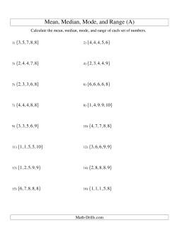
Calculating the mean, median, mode and range are staples of the upper elementary math curriculum. Here you will find worksheets for practicing the calculation of mean, median, mode and range. In case you're not familiar with these concepts, here is how to calculate each one. To calculate the mean, add all of the numbers in the set together and divide that sum by the number of numbers in the set. To calculate the median, first arrange the numbers in order, then locate the middle number. In sets where there are an even number of numbers, calculate the mean of the two middle numbers. To calculate the mode, look for numbers that repeat. If there is only one of each number, the set has no mode. If there are doubles of two different numbers and there are more numbers in the set, the set has two modes. If there are triples of three different numbers and there are more numbers in the set, the set has three modes, and so on. The range is calculated by subtracting the least number from the greatest number.

Note that all of the measures of central tendency are included on each page, but you don't need to assign them all if you aren't working on them all. If you're only working on mean, only assign students to calculate the mean.

In order to determine the median, it is necessary to have your numbers sorted. It is also helpful in determining the mode and range. To expedite the process, these first worksheets include the lists of numbers already sorted.

• Calculating Mean, Median, Mode and Range from Sorted Lists Sets of 5 Numbers from 1 to 10 Sets of 5 Numbers from 10 to 99 Sets of 5 Numbers from 100 to 999 Sets of 10 Numbers from 1 to 10 Sets of 10 Numbers from 10 to 99 Sets of 10 Numbers from 100 to 999 Sets of 20 Numbers from 10 to 99 Sets of 15 Numbers from 100 to 999

Normally, data does not come in a sorted list, so these worksheets are a little more realistic. To find some of the statistics, it will be easier for students to put the numbers in order first.

• Calculating Mean, Median, Mode and Range from Unsorted Lists Sets of 5 Numbers from 1 to 10 Sets of 5 Numbers from 10 to 99 Sets of 5 Numbers from 100 to 999 Sets of 10 Numbers from 1 to 10 Sets of 10 Numbers from 10 to 99 Sets of 10 Numbers from 100 to 999 Sets of 20 Numbers from 10 to 99 Sets of 15 Numbers from 100 to 999

Collecting and Organizing Data

Teaching students how to collect and organize data enables them to develop skills that will enable them to study topics in statistics with more confidence and deeper understanding.

• Constructing Line Plots from Small Data Sets Construct Line Plots with Smaller Numbers and Lines with Ticks Provided (Small Data Set) Construct Line Plots with Smaller Numbers and Lines Only Provided (Small Data Set) Construct Line Plots with Smaller Numbers (Small Data Set) Construct Line Plots with Larger Numbers and Lines with Ticks Provided (Small Data Set) Construct Line Plots with Larger Numbers and Lines Only Provided (Small Data Set) Construct Line Plots with Larger Numbers (Small Data Set)
• Constructing Line Plots from Larger Data Sets Construct Line Plots with Smaller Numbers and Lines with Ticks Provided Construct Line Plots with Smaller Numbers and Lines Only Provided Construct Line Plots with Smaller Numbers Construct Line Plots with Larger Numbers and Lines with Ticks Provided Construct Line Plots with Larger Numbers and Lines Only Provided Construct Line Plots with Larger Numbers

Interpreting and Analyzing Data

Answering questions about graphs and other data helps students build critical thinking skills. Standard questions include determining the minimum, maximum, range, count, median, mode, and mean.

• Answering Questions About Stem-and-Leaf Plots Stem-and-Leaf Plots with about 25 data points Stem-and-Leaf Plots with about 50 data points Stem-and-Leaf Plots with about 100 data points
• Answering Questions About Line Plots Line Plots with Smaller Data Sets and Smaller Numbers Line Plots with Smaller Data Sets and Larger Numbers Line Plots with Larger Data Sets and Smaller Numbers Line Plots with Larger Data Sets and Larger Numbers
• Answering Questions About Broken-Line Graphs Answer Questions About Broken-Line Graphs
• Answering Questions About Circle Graphs Circle Graph Questions (Color Version) Circle Graph Questions (Black and White Version) Circle Graphs No Questions (Color Version) Circle Graphs No Questions (Black and White Version)
• Answering Questions About Pictographs Answer Questions About Pictographs

Probability Worksheets

• Calculating Probabilities with Dice Sum of Two Dice Probabilities Sum of Two Dice Probabilities (with table)

Spinners can be used for probability experiments or for theoretical probability. Students should intuitively know that a number that is more common on a spinner will come up more often. Spinning 100 or more times and tallying the results should get them close to the theoretical probability. The more sections there are, the more spins will be needed.

• Calculating Probabilities with Number Spinners Number Spinner Probability (4 Sections) Number Spinner Probability (5 Sections) Number Spinner Probability (6 Sections) Number Spinner Probability (7 Sections) Number Spinner Probability (8 Sections) Number Spinner Probability (9 Sections) Number Spinner Probability (10 Sections) Number Spinner Probability (11 Sections) Number Spinner Probability (12 Sections)

Non-numerical spinners can be used for experimental or theoretical probability. There are basic questions on every version with a couple extra questions on the A and B versions. Teachers and students can make up other questions to ask and conduct experiments or calculate the theoretical probability. Print copies for everyone or display on an interactive white board.

• Probability with Single-Event Spinners Animal Spinner Probability ( 4 Sections) Animal Spinner Probability ( 5 Sections) Animal Spinner Probability ( 10 Sections) Letter Spinner Probability ( 4 Sections) Letter Spinner Probability ( 5 Sections) Letter Spinner Probability ( 10 Sections) Color Spinner Probability ( 4 Sections) Color Spinner Probability ( 5 Sections) Color Spinner Probability ( 10 Sections)
• Probability with Multi-Event Spinners Animal/Letter Combined Spinner Probability ( 4 Sections) Animal/Letter Combined Spinner Probability ( 5 Sections) Animal/Letter Combined Spinner Probability ( 10 Sections) Animal/Letter/Color Combined Spinner Probability ( 4 Sections) Animal/Letter/Color Combined Spinner Probability ( 5 Sections) Animal/Letter/Color Combined Spinner Probability ( 10 Sections)

Copyright © 2005-2024 Math-Drills.com You may use the math worksheets on this website according to our Terms of Use to help students learn math.

11 Surprising Homework Statistics, Facts & Data

The age-old question of whether homework is good or bad for students is unanswerable because there are so many “ it depends ” factors.

For example, it depends on the age of the child, the type of homework being assigned, and even the child’s needs.

There are also many conflicting reports on whether homework is good or bad. This is a topic that largely relies on data interpretation for the researcher to come to their conclusions.

To cut through some of the fog, below I’ve outlined some great homework statistics that can help us understand the effects of homework on children.

Homework Statistics List

1. 45% of parents think homework is too easy for their children.

A study by the Center for American Progress found that parents are almost twice as likely to believe their children’s homework is too easy than to disagree with that statement.

Here are the figures for math homework:

• 46% of parents think their child’s math homework is too easy.
• 25% of parents think their child’s math homework is not too easy.
• 29% of parents offered no opinion.

Here are the figures for language arts homework:

• 44% of parents think their child’s language arts homework is too easy.
• 28% of parents think their child’s language arts homework is not too easy.
• 28% of parents offered no opinion.

These findings are based on online surveys of 372 parents of school-aged children conducted in 2018.

2. 93% of Fourth Grade Children Worldwide are Assigned Homework

The prestigious worldwide math assessment Trends in International Maths and Science Study (TIMSS) took a survey of worldwide homework trends in 2007. Their study concluded that 93% of fourth-grade children are regularly assigned homework, while just 7% never or rarely have homework assigned.

3. 17% of Teens Regularly Miss Homework due to Lack of High-Speed Internet Access

A 2018 Pew Research poll of 743 US teens found that 17%, or almost 2 in every 5 students, regularly struggled to complete homework because they didn’t have reliable access to the internet.

This figure rose to 25% of Black American teens and 24% of teens whose families have an income of less than $30,000 per year.

4. Parents Spend 6.7 Hours Per Week on their Children’s Homework

A 2018 study of 27,500 parents around the world found that the average amount of time parents spend on homework with their child is 6.7 hours per week. Furthermore, 25% of parents spend more than 7 hours per week on their child’s homework.

American parents spend slightly below average at 6.2 hours per week, while Indian parents spend 12 hours per week and Japanese parents spend 2.6 hours per week.

5. Students in High-Performing High Schools Spend on Average 3.1 Hours per night Doing Homework

A study by Galloway, Conner & Pope (2013) conducted a sample of 4,317 students from 10 high-performing high schools in upper-middle-class California. 

Across these high-performing schools, students self-reported that they did 3.1 hours per night of homework.

Graduates from those schools also ended up going on to college 93% of the time.

6. One to Two Hours is the Optimal Duration for Homework

A 2012 peer-reviewed study in the High School Journal found that students who conducted between one and two hours achieved higher results in tests than any other group.

However, the authors were quick to highlight that this “t is an oversimplification of a much more complex problem.” I’m inclined to agree. The greater variable is likely the quality of the homework than time spent on it.

Nevertheless, one result was unequivocal: that some homework is better than none at all : “students who complete any amount of homework earn higher test scores than their peers who do not complete homework.”

7. 74% of Teens cite Homework as a Source of Stress

A study by the Better Sleep Council found that homework is a source of stress for 74% of students. Only school grades, at 75%, rated higher in the study.

That figure rises for girls, with 80% of girls citing homework as a source of stress.

Similarly, the study by Galloway, Conner & Pope (2013) found that 56% of students cite homework as a “primary stressor” in their lives.

8. US Teens Spend more than 15 Hours per Week on Homework

The same study by the Better Sleep Council also found that US teens spend over 2 hours per school night on homework, and overall this added up to over 15 hours per week.

Surprisingly, 4% of US teens say they do more than 6 hours of homework per night. That’s almost as much homework as there are hours in the school day.

The only activity that teens self-reported as doing more than homework was engaging in electronics, which included using phones, playing video games, and watching TV.

9. The 10-Minute Rule

The National Education Association (USA) endorses the concept of doing 10 minutes of homework per night per grade.

For example, if you are in 3rd grade, you should do 30 minutes of homework per night. If you are in 4th grade, you should do 40 minutes of homework per night.

However, this ‘rule’ appears not to be based in sound research. Nevertheless, it is true that homework benefits (no matter the quality of the homework) will likely wane after 2 hours (120 minutes) per night, which would be the NEA guidelines’ peak in grade 12.

10. 21.9% of Parents are Too Busy for their Children’s Homework

An online poll of nearly 300 parents found that 21.9% are too busy to review their children’s homework. On top of this, 31.6% of parents do not look at their children’s homework because their children do not want their help. For these parents, their children’s unwillingness to accept their support is a key source of frustration.

11. 46.5% of Parents find Homework too Hard

The same online poll of parents of children from grades 1 to 12 also found that many parents struggle to help their children with homework because parents find it confusing themselves. Unfortunately, the study did not ask the age of the students so more data is required here to get a full picture of the issue.

Get a Pdf of this article for class

Enjoy subscriber-only access to this article’s pdf

Interpreting the Data

Unfortunately, homework is one of those topics that can be interpreted by different people pursuing differing agendas. All studies of homework have a wide range of variables, such as:

• What age were the children in the study?
• What was the homework they were assigned?
• What tools were available to them?
• What were the cultural attitudes to homework and how did they impact the study?
• Is the study replicable?

The more questions we ask about the data, the more we realize that it’s hard to come to firm conclusions about the pros and cons of homework .

Furthermore, questions about the opportunity cost of homework remain. Even if homework is good for children’s test scores, is it worthwhile if the children consequently do less exercise or experience more stress?

Thus, this ends up becoming a largely qualitative exercise. If parents and teachers zoom in on an individual child’s needs, they’ll be able to more effectively understand how much homework a child needs as well as the type of homework they should be assigned.

Related: Funny Homework Excuses

The debate over whether homework should be banned will not be resolved with these homework statistics. But, these facts and figures can help you to pursue a position in a school debate on the topic – and with that, I hope your debate goes well and you develop some great debating skills!

Chris Drew (PhD)

Dr. Chris Drew is the founder of the Helpful Professor. He holds a PhD in education and has published over 20 articles in scholarly journals. He is the former editor of the Journal of Learning Development in Higher Education. [Image Descriptor: Photo of Chris]

• Chris Drew (PhD) https://helpfulprofessor.com/author/chris-drew-phd/ 10 Elaborative Rehearsal Examples
• Chris Drew (PhD) https://helpfulprofessor.com/author/chris-drew-phd/ Maintenance Rehearsal - Definition & Examples
• Chris Drew (PhD) https://helpfulprofessor.com/author/chris-drew-phd/ Piaget vs Vygotsky: Similarities and Differences
• Chris Drew (PhD) https://helpfulprofessor.com/author/chris-drew-phd/ 10 Conditioned Response Examples

Leave a Comment Cancel Reply

Your email address will not be published. Required fields are marked *

CSE 163, Summer 2020: Homework 3: Data Analysis

In this assignment, you will apply what you've learned so far in a more extensive "real-world" dataset using more powerful features of the Pandas library. As in HW2, this dataset is provided in CSV format. We have cleaned up the data some, but you will need to handle more edge cases common to real-world datasets, including null cells to represent unknown information.

Note that there is no graded testing portion of this assignment. We still recommend writing tests to verify the correctness of the methods that you write in Part 0, but it will be difficult to write tests for Part 1 and 2. We've provided tips in those sections to help you gain confidence about the correctness of your solutions without writing formal test functions!

This assignment is supposed to introduce you to various parts of the data science process involving being able to answer questions about your data, how to visualize your data, and how to use your data to make predictions for new data. To help prepare for your final project, this assignment has been designed to be wide in scope so you can get practice with many different aspects of data analysis. While this assignment might look large because there are many parts, each individual part is relatively small.

Learning Objectives

After this homework, students will be able to:

• Work with basic Python data structures.
• Handle edge cases appropriately, including addressing missing values/data.
• Practice user-friendly error-handling.
• Read plotting library documentation and use example plotting code to figure out how to create more complex Seaborn plots.
• Train a machine learning model and use it to make a prediction about the future using the scikit-learn library.

Expectations

Here are some baseline expectations we expect you to meet:

Follow the course collaboration policies

If you are developing on Ed, all the files are there. The files included are:

• hw3-nces-ed-attainment.csv : A CSV file that contains data from the National Center for Education Statistics. This is described in more detail below.
• hw3.py : The file for you to put solutions to Part 0, Part 1, and Part 2. You are required to add a main method that parses the provided dataset and calls all of the functions you are to write for this homework.
• hw3-written.txt : The file for you to put your answers to the questions in Part 3.
• cse163_utils.py : Provides utility functions for this assignment. You probably don't need to use anything inside this file except importing it if you have a Mac (see comment in hw3.py )

If you are developing locally, you should navigate to Ed and in the assignment view open the file explorer (on the left). Once there, you can right-click to select the option to "Download All" to download a zip and open it as the project in Visual Studio Code.

The dataset you will be processing comes from the National Center for Education Statistics. You can find the original dataset here . We have cleaned it a bit to make it easier to process in the context of this assignment. You must use our provided CSV file in this assignment.

The original dataset is titled: Percentage of persons 25 to 29 years old with selected levels of educational attainment, by race/ethnicity and sex: Selected years, 1920 through 2018 . The cleaned version you will be working with has columns for Year, Sex, Educational Attainment, and race/ethnicity categories considered in the dataset. Note that not all columns will have data starting at 1920.

Our provided hw3-nces-ed-attainment.csv looks like: (⋮ represents omitted rows):

Column Descriptions

• Year: The year this row represents. Note there may be more than one row for the same year to show the percent breakdowns by sex.
• Sex: The sex of the students this row pertains to, one of "F" for female, "M" for male, or "A" for all students.
• Min degree: The degree this row pertains to. One of "high school", "associate's", "bachelor's", or "master's".
• Total: The total percent of students of the specified gender to reach at least the minimum level of educational attainment in this year.
• White / Black / Hispanic / Asian / Pacific Islander / American Indian or Alaska Native / Two or more races: The percent of students of this race and the specified gender to reach at least the minimum level of educational attainment in this year.

Interactive Development

When using data science libraries like pandas , seaborn , or scikit-learn it's extremely helpful to actually interact with the tools your using so you can have a better idea about the shape of your data. The preferred practice by people in industry is to use a Jupyter Notebook, like we have been in lecture, to play around with the dataset to help figure out how to answer the questions you want to answer. This is incredibly helpful when you're first learning a tool as you can actually experiment and get real-time feedback if the code you wrote does what you want.

We recommend that you try figuring out how to solve these problems in a Jupyter Notebook so you can actually interact with the data. We have made a Playground Jupyter Notebook for you that has the data uploaded. At the top-right of this page in Ed is a "Fork" button (looks like a fork in the road). This will make your own copy of this Notebook so you can run the code and experiment with anything there! When you open the Workspace, you should see a list of notebooks and CSV files. You can always access this launch page by clicking the Jupyter logo.

Part 0: Statistical Functions with Pandas

In this part of the homework, you will write code to perform various analytical operations on data parsed from a file.

Part 0 Expectations

• All functions for this part of the assignment should be written in hw3.py .
• For this part of the assignment, you may import and use the math and pandas modules, but you may not use any other imports to solve these problems.
• For all of the problems below, you should not use ANY loops or list/dictionary comprehensions. The goal of this part of the assignment is to use pandas as a tool to help answer questions about your dataset.

Problem 0: Parse data

In your main method, parse the data from the CSV file using pandas. Note that the file uses '---' as the entry to represent missing data. You do NOT need to anything fancy like set a datetime index.

The function to read a CSV file in pandas takes a parameter called na_values that takes a str to specify which values are NaN values in the file. It will replace all occurrences of those characters with NaN. You should specify this parameter to make sure the data parses correctly.

Problem 1: compare_bachelors_1980

What were the percentages for women vs. men having earned a Bachelor's Degree in 1980? Call this method compare_bachelors_1980 and return the result as a DataFrame with a row for men and a row for women with the columns "Sex" and "Total".

The index of the DataFrame is shown as the left-most column above.

Problem 2: top_2_2000s

What were the two most commonly awarded levels of educational attainment awarded between 2000-2010 (inclusive)? Use the mean percent over the years to compare the education levels in order to find the two largest. For this computation, you should use the rows for the 'A' sex. Call this method top_2_2000s and return a Series with the top two values (the index should be the degree names and the values should be the percent).

For example, assuming we have parsed hw3-nces-ed-attainment.csv and stored it in a variable called data , then top_2_2000s(data) will return the following Series (shows the index on the left, then the value on the right)

Hint: The Series class also has a method nlargest that behaves similarly to the one for the DataFrame , but does not take a column parameter (as Series objects don't have columns).

Our assert_equals only checks that floating point numbers are within 0.001 of each other, so your floats do not have to match exactly.

Optional: Why 0.001?

Whenever you work with floating point numbers, it is very likely you will run into imprecision of floating point arithmetic . You have probably run into this with your every day calculator! If you take 1, divide by 3, and then multiply by 3 again you could get something like 0.99999999 instead of 1 like you would expect.

This is due to the fact that there is only a finite number of bits to represent floats so we will at some point lose some precision. Below, we show some example Python expressions that give imprecise results.

Because of this, you can never safely check if one float is == to another. Instead, we only check that the numbers match within some small delta that is permissible by the application. We kind of arbitrarily chose 0.001, and if you need really high accuracy you would want to only allow for smaller deviations, but equality is never guaranteed.

Problem 3: percent_change_bachelors_2000s

What is the difference between total percent of bachelor's degrees received in 2000 as compared to 2010? Take a sex parameter so the client can specify 'M', 'F', or 'A' for evaluating. If a call does not specify the sex to evaluate, you should evaluate the percent change for all students (sex = ‘A’). Call this method percent_change_bachelors_2000s and return the difference (the percent in 2010 minus the percent in 2000) as a float.

For example, assuming we have parsed hw3-nces-ed-attainment.csv and stored it in a variable called data , then the call percent_change_bachelors_2000s(data) will return 2.599999999999998 . Our assert_equals only checks that floating point numbers are within 0.001 of each other, so your floats do not have to match exactly.

Hint: For this problem you will need to use the squeeze() function on a Series to get a single value from a Series of length 1.

Part 1: Plotting with Seaborn

Next, you will write functions to generate data visualizations using the Seaborn library. For each of the functions save the generated graph with the specified name. These methods should only take the pandas DataFrame as a parameter. For each problem, only drop rows that have missing data in the columns that are necessary for plotting that problem ( do not drop any additional rows ).

Part 1 Expectations

• When submitting on Ed, you DO NOT need to specify the absolute path (e.g. /home/FILE_NAME ) for the output file name. If you specify absolute paths for this assignment your code will not pass the tests!
• You will want to pass the parameter value bbox_inches='tight' to the call to savefig to make sure edges of the image look correct!
• For this part of the assignment, you may import the math , pandas , seaborn , and matplotlib modules, but you may not use any other imports to solve these problems.
• For all of the problems below, you should not use ANY loops or list/dictionary comprehensions.
• Do not use any of the other seaborn plotting functions for this assignment besides the ones we showed in the reference box below. For example, even though the documentation for relplot links to another method called scatterplot , you should not call scatterplot . Instead use relplot(..., kind='scatter') like we showed in class. This is not an issue of stylistic preference, but these functions behave slightly differently. If you use these other functions, your output might look different than the expected picture. You don't yet have the tools necessary to use scatterplot correctly! We will see these extra tools later in the quarter.

Part 1 Development Strategy

• Print your filtered DataFrame before creating the graph to ensure you’re selecting the correct data.
• Call the DataFrame describe() method to see some statistical information about the data you've selected. This can sometimes help you determine what to expect in your generated graph.
• Re-read the problem statement to make sure your generated graph is answering the correct question.
• Compare the data on your graph to the values in hw3-nces-ed-attainment.csv. For example, for problem 0 you could check that the generated line goes through the point (2005, 28.8) because of this row in the dataset: 2005,A,bachelor's,28.8,34.5,17.6,11.2,62.1,17.0,16.4,28.0

Seaborn Reference

Of all the libraries we will learn this quarter, Seaborn is by far the best documented. We want to give you experience reading real world documentation to learn how to use a library so we will not be providing a specialized cheat-sheet for this assignment. What we will do to make sure you don't have to look through pages and pages of documentation is link you to some key pages you might find helpful for this assignment; you do not have to use every page we link, so part of the challenge here is figuring out which of these pages you need. As a data scientist, a huge part of solving a problem is learning how to skim lots of documentation for a tool that you might be able to leverage to solve your problem.

We recommend to read the documentation in the following order:

• Start by skimming the examples to see the possible things the function can do. Don't spend too much time trying to figure out what the code is doing yet, but you can quickly look at it to see how much work is involved.
• Then read the top paragraph(s) that give a general overview of what the function does.
• Now that you have a better idea of what the function is doing, go look back at the examples and look at the code much more carefully. When you see an example like the one you want to generate, look carefully at the parameters it passes and go check the parameter list near the top for documentation on those parameters.
• It sometimes (but not always), helps to skim the other parameters in the list just so you have an idea what this function is capable of doing

As a reminder, you will want to refer to the lecture/section material to see the additional matplotlib calls you might need in order to display/save the plots. You'll also need to call the set function on seaborn to get everything set up initially.

Here are the seaborn functions you might need for this assignment:

• Bar/Violin Plot ( catplot )
• Plot a Discrete Distribution ( distplot ) or Continuous Distribution ( kdeplot )
• Scatter/Line Plot ( relplot )
• Linear Regression Plot ( regplot )
• Compare Two Variables ( jointplot )
• Heatmap ( heatmap )

Make sure you read the bullet point at the top of the page warning you to only use these functions!

Problem 0: Line Chart

Plot the total percentages of all people of bachelor's degree as minimal completion with a line chart over years. To select all people, you should filter to rows where sex is 'A'. Label the x-axis "Year", the y-axis "Percentage", and title the plot "Percentage Earning Bachelor's over Time". Name your method line_plot_bachelors and save your generated graph as line_plot_bachelors.png .

Problem 1: Bar Chart

Plot the total percentages of women, men, and total people with a minimum education of high school degrees in the year 2009. Label the x-axis "Sex", the y-axis "Percentage", and title the plot "Percentage Completed High School by Sex". Name your method bar_chart_high_school and save your generated graph as bar_chart_high_school.png .

Do you think this bar chart is an effective data visualization? Include your reasoning in hw3-written.txt as described in Part 3.

Problem 2: Custom Plot

Plot the results of how the percent of Hispanic individuals with degrees has changed between 1990 and 2010 (inclusive) for high school and bachelor's degrees with a chart of your choice. Make sure you label your axes with descriptive names and give a title to the graph. Name your method plot_hispanic_min_degree and save your visualization as plot_hispanic_min_degree.png .

Include a justification of your choice of data visualization in hw3-written.txt , as described in Part 3.

Part 2: Machine Learning using scikit-learn

Now you will be making a simple machine learning model for the provided education data using scikit-learn . Complete this in a function called fit_and_predict_degrees that takes the data as a parameter and returns the test mean squared error as a float. This may sound like a lot, so we've broken it down into steps for you:

• Filter the DataFrame to only include the columns for year, degree type, sex, and total.
• Do the following pre-processing: Drop rows that have missing data for just the columns we are using; do not drop any additional rows . Convert string values to their one-hot encoding. Split the columns as needed into input features and labels.
• Randomly split the dataset into 80% for training and 20% for testing.
• Train a decision tree regressor model to take in year, degree type, and sex to predict the percent of individuals of the specified sex to achieve that degree type in the specified year.
• Use your model to predict on the test set. Calculate the accuracy of your predictions using the mean squared error of the test dataset.

You do not need to anything fancy like find the optimal settings for parameters to maximize performance. We just want you to start simple and train a model from scratch! The reference below has all the methods you will need for this section!

scikit-learn Reference

You can find our reference sheet for machine learning with scikit-learn ScikitLearnReference . This reference sheet has information about general scikit-learn calls that are helpful, as well as how to train the tree models we talked about in class. At the top-right of this page in Ed is a "Fork" button (looks like a fork in the road). This will make your own copy of this Notebook so you can run the code and experiment with anything there! When you open the Workspace, you should see a list of notebooks and CSV files. You can always access this launch page by clikcing the Jupyter logo.

Part 2 Development Strategy

Like in Part 1, it can be difficult to write tests for this section. Machine Learning is all about uncertainty, and it's often difficult to write tests to know what is right. This requires diligence and making sure you are very careful with the method calls you make. To help you with this, we've provided some alternative ways to gain confidence in your result:

• Print your test y values and your predictions to compare them manually. They won't be exactly the same, but you should notice that they have some correlation. For example, I might be concerned if my test y values were [2, 755, …] and my predicted values were [1022, 5...] because they seem to not correlate at all.
• Calculate your mean squared error on your training data as well as your test data. The error should be lower on your training data than on your testing data.

Optional: ML for Time Series

Since this is technically time series data, we should point out that our method for assessing the model's accuracy is slightly wrong (but we will keep it simple for our HW). When working with time series, it is common to use the last rows for your test set rather than random sampling (assuming your data is sorted chronologically). The reason is when working with time series data in machine learning, it's common that our goal is to make a model to help predict the future. By randomly sampling a test set, we are assessing the model on its ability to predict in the past! This is because it might have trained on rows that came after some rows in the test set chronologically. However, this is not a task we particularly care that the model does well at. Instead, by using the last section of the dataset (the most recent in terms of time), we are now assessing its ability to predict into the future from the perspective of its training set.

Even though it's not the best approach to randomly sample here, we ask you to do it anyways. This is because random sampling is the most common method for all other data types.

Part 3: Written Responses

Review the source of the dataset here . For the following reflection questions consider the accuracy of data collected, and how it's used as a public dataset (e.g. presentation of data, publishing in media, etc.). All of your answers should be complete sentences and show thoughtful responses. "No" or "I don't know" or any response like that are not valid responses for any questions. There is not one particularly right answer to these questions, instead, we are looking to see you use your critical thinking and justify your answers!

• Do you think the bar chart from part 1b is an effective data visualization? Explain in 1-2 sentences why or why not.
• Why did you choose the type of plot that you did in part 1c? Explain in a few sentences why you chose this type of plot.
• Datasets can be biased. Bias in data means it might be skewed away from or portray a wrong picture of reality. The data might contain inaccuracies or the methods used to collect the data may have been flawed. Describe a possible bias present in this dataset and why it might have occurred. Your answer should be about 2 or 3 sentences long.

Context : Later in the quarter we will talk about ethics and data science. This question is supposed to be a warm-up to get you thinking about our responsibilities having this power to process data. We are not trying to train to misuse your powers for evil here! Most misuses of data analysis that result in ethical concerns happen unintentionally. As preparation to understand these unintentional consequences, we thought it would be a good exercise to think about a theoretical world where you would willingly try to misuse data.

Congrats! You just got an internship at Evil Corp! Your first task is to come up with an application or analysis that uses this dataset to do something unethical or nefarious. Describe a way that this dataset could be misused in some application or an analysis (potentially using the bias you identified for the last question). Regardless of what nefarious act you choose, evil still has rules: You need to justify why using the data in this is a misuse and why a regular person who is not evil (like you in the real world outside of this problem) would think using the data in this way would be wrong. There are no right answers here of what defines something as unethical, this is why you need to justify your answer! Your response should be 2 to 4 sentences long.

Turn your answers to these question in by writing them in hw3-written.txt and submitting them on Ed

Your submission will be evaluated on the following dimensions:

• Your solution correctly implements the described behaviors. You will have access to some tests when you turn in your assignment, but we will withhold other tests to test your solution when grading. All behavior we test is completely described by the problem specification or shown in an example.
• No method should modify its input parameters.
• Your main method in hw3.py must call every one of the methods you implemented in this assignment. There are no requirements on the format of the output, besides that it should save the files for Part 1 with the proper names specified in Part 1.
• We can run your hw3.py without it crashing or causing any errors or warnings.
• When we run your code, it should produce no errors or warnings.
• All files submitted pass flake8
• All program files should be written with good programming style. This means your code should satisfy the requirements within the CSE 163 Code Quality Guide .
• Any expectations on this page or the sub-pages for the assignment are met as well as all requirements for each of the problems are met.

Make sure you carefully read the bullets above as they may or may not change from assignment to assignment!

A note on allowed material

A lot of students have been asking questions like "Can I use this method or can I use this language feature in this class?". The general answer to this question is it depends on what you want to use, what the problem is asking you to do and if there are any restrictions that problem places on your solution.

There is no automatic deduction for using some advanced feature or using material that we have not covered in class yet, but if it violates the restrictions of the assignment, it is possible you will lose points. It's not possible for us to list out every possible thing you can't use on the assignment, but we can say for sure that you are safe to use anything we have covered in class so far as long as it meets what the specification asks and you are appropriately using it as we showed in class.

For example, some things that are probably okay to use even though we didn't cover them:

• Using the update method on the set class even though I didn't show it in lecture. It was clear we talked about sets and that you are allowed to use them on future assignments and if you found a method on them that does what you need, it's probably fine as long as it isn't violating some explicit restriction on that assignment.
• Using something like a ternary operator in Python. This doesn't make a problem any easier, it's just syntax.

For example, some things that are probably not okay to use:

• Importing some random library that can solve the problem we ask you to solve in one line.
• If the problem says "don't use a loop" to solve it, it would not be appropriate to use some advanced programming concept like recursion to "get around" that restriction.

These are not allowed because they might make the problem trivially easy or violate what the learning objective of the problem is.

You should think about what the spec is asking you to do and as long as you are meeting those requirements, we will award credit. If you are concerned that an advanced feature you want to use falls in that second category above and might cost you points, then you should just not use it! These problems are designed to be solvable with the material we have learned so far so it's entirely not necessary to go look up a bunch of advanced material to solve them.

tl;dr; We will not be answering every question of "Can I use X" or "Will I lose points if I use Y" because the general answer is "You are not forbidden from using anything as long as it meets the spec requirements. If you're unsure if it violates a spec restriction, don't use it and just stick to what we learned before the assignment was released."

This assignment is due by Thursday, July 23 at 23:59 (PDT) .

You should submit your finished hw3.py , and hw3-written.txt on Ed .

You may submit your assignment as many times as you want before the late cutoff (remember submitting after the due date will cost late days). Recall on Ed, you submit by pressing the "Mark" button. You are welcome to develop the assignment on Ed or develop locally and then upload to Ed before marking.

• Skip to main content

Maneuvering the Middle

Student-Centered Math Lessons

• All Products

Data and Statistics Unit 7th Grade CCSS

A 9 day CCSS-Aligned Statistics Unit – including populations and samples, drawing inferences from samples, measures of centers and variability, comparing and analyzing dot and box plots.

Description

Additional information.

• Reviews (0)

Students will practice with both skill-based problems, real-world application questions, and error analysis to support higher level thinking skills.  You can reach your students and teach the standards without all of the prep and stress of creating materials!

Standards:   7.SP.1, 7.SP.2, 7.SP.3, 7.SP.4;  Texas Teacher?  Grab the TEKS-Aligned Statistics Unit.   Please don’t purchase both as there is overlapping content.

Learning Focus:

• compare two populations based on random samples and use data to make inferences
• determine measures of center and variability
• compare the shapes, centers, and spreads of dot plots and box plots

What is included in the 7th grade ccss Data and Statistics Unit?

1. Unit Overviews

• Streamline planning with unit overviews that include essential questions, big ideas, vertical alignment, vocabulary, and common misconceptions.
• A pacing guide and tips for teaching each topic are included to help you be more efficient in your planning.

2. Student Handouts

• Student-friendly guided notes are scaffolded to support student learning.
• Available as a PDF and the student handouts/homework/study guides have been converted to Google Slides™ for your convenience.

3. Independent Practice

• Daily homework is aligned directly to the student handouts and is versatile for both in class or at home practice.

4. Assessments

• 1-2 quizzes, a unit study guide, and a unit test allow you to easily assess and meet the needs of your students.
• The Unit Test is available as an editable PPT, so that you can modify and adjust questions as needed.

5. Answer Keys

• All answer keys are included.

***Please download a preview to see sample pages and more information.***

How to use this resource:

• Use as a whole group, guided notes setting
• Use in a small group, math workshop setting
• Chunk each student handout to incorporate whole group instruction, small group practice, and independent practice.
• Incorporate our  Statistics Activity Bundle  for hands-on activities as additional and engaging practice opportunities.

Time to Complete:

• Each student handout is designed for a single class period. However, feel free to review the problems and select specific ones to meet your student needs. There are multiple problems to practice the same concepts, so you can adjust as needed.

Is this resource editable?

• The unit test is editable with Microsoft PPT. The remainder of the file is a PDF and not editable.

Looking for more 7 th Grade Math Material? Join our All Access Membership Community! You can reach your students without the “I still have to prep for tomorrow” stress, the constant overwhelm of teaching multiple preps, and the hamster wheel demands of creating your own teaching materials.

• Grade Level Curriculum
• Supplemental Digital Components
• Complete and Comprehensive Student Video Library 

Click here to learn more about All Access by Maneuvering the Middle®!

Licensing: This file is a license for ONE teacher and their students. Please purchase the appropriate number of licenses if you plan to use this resource with your team. Thank you!

Customer Service: If you have any questions, please feel free to reach out for assistance .  We aim to provide quality resources to help teachers and students alike, so please reach out if you have any questions or concerns. 

Maneuvering the Middle ® Terms of Use: Products by Maneuvering the Middle®, LLC may be used by the purchaser for their classroom use only. This is a single classroom license only. All rights reserved. Resources may only be posted online in an LMS such as Google Classroom, Canvas, or Schoology. Students should be the only ones able to access the resources.  It is a copyright violation to upload the files to school/district servers or shared Google Drives. See more information on our terms of use here . 

If you are interested in a personalized quote for campus and district licenses, please click here . 

©Maneuvering the Middle® LLC, 2012-present

This file is a license for one teacher and their students. Please purchase the appropriate number of licenses if you plan to use this resource with your team. Thank you!

Customer Service

We strive to provide quality products to help teachers and students alike, so contact us with any questions.

Maneuvering the Middle® Terms of Use

Products by Maneuvering the Middle, LLC may be used by the purchaser for their classroom use only. This is a single classroom license only. All rights reserved. Resources may only be posted online if they are behind a password-protected site.

Campus and district licensing is available please contact us for pricing.

©Maneuvering the Middle LLC, 2012-present

There are no reviews yet.

Only logged in customers who have purchased this product may leave a review.

This resource is often paired with:

Data and Statistics Unit 7th Grade TEKS

Statistics Activity Bundle 7th Grade

Digital Math Activity Bundle 7th Grade

Algeria: Investing in Data Key for Diversified Growth

The Spring 2024 Algeria Economic Update underlines the country’s dynamic economic activity and slowing inflation while highlighting the importance of data in supporting Algeria’s efforts toward sustainable, diversified growth.

ALGIERS, May 22, 2024 —  Algeria’s economic growth remained dynamic in 2023, with GDP recording a 4.1 percent increase, driven by robust performance in the nonhydrocarbon and hydrocarbon sectors, according to the World Bank's Spring 2024 Algeria Economic Update . Economic activity was stimulated by dynamic private consumption and strong investment growth, fueling a marked increase in imports. Hydrocarbon production was supported by record-high natural gas production, compensating for the decline in crude oil production amidst voluntary OPEC quota reductions.

Despite the decline in global hydrocarbon prices and an increase in imports causing Algeria’s’ trade balance to shrink, the country's foreign reserves continued to increase, reaching a comfortable 16.1 months of imports by the end of 2023. Consumer price inflation moderated to 5.0 percent in the first quarter of 2024, down from 9.3 percent in 2023, aided by a strong dinar and a decrease in fresh food and import prices. 

The report underscores the strategic importance of data in informing policy decisions and the potential to leverage alternative data sources to shed light on real-time economic developments in Algeria. These sources, such as satellite data on nighttime lights, crop development, as well as data on shipping vessels arriving at and departing from Algerian ports, can provide a more detailed view of the economy. The report looks at how these data sources represent a useful complement to conventional economic and social statistics while stressing that improving the availability, granularity, and timeliness of official economic data, most notably relating to activity, investment, and the labor market, remains of utmost importance.

"In 2022 and 2023, Algerian authorities accelerated digitalization efforts and elevated the strengthening of data systems as a policy priority,” said Kamel Braham, the World Bank’s Resident Representative to Algeria . “In addition to supporting evidence-based policymaking, robust economic data reduces economic uncertainty and supports investment, growth, and diversification.”

Looking ahead, the report projects a temporary growth slowdown in 2024, followed by a robust recovery in 2025. Despite the positive outlook it finds that continued public spending and import growth amidst moderating hydrocarbon exports would put renewed pressure on the fiscal and trade balances. Additionally, significant uncertainties with respect to global commodity prices and climate conditions remain. 

Cyril Desponts, the World Bank’s Senior Economist for Algeria , underlined the usefulness of alternative data sources, “Unconventional data bring precision to our analysis because they are highly disaggregated across time and space, and available with only a short delay. In early 2024, data suggest that activity remained dynamic across the country, but to a lesser extent in oil-producing regions, affected by quota reductions and that Eastern regions saw a recovery in rainfall and crop development, feeding into our macroeconomic projections.”

The report also highlights the significance of recent reforms and the importance of supporting diversification by accelerating private sector investment in non-hydrocarbon sectors. The 2022 Investment Law, the 2023 Banking and Monetary Law, formal adhesion to the Africa Continental Free Trade Agreement, the 2023 Land Law, and initiation of state-owned bank reforms are all aimed at boosting private investment to foster diversification. Strengthening these efforts is even more important now that public investment, previously the engine of Algeria’s growth, is increasingly constrained by expanding current expenditures.

This site uses cookies to optimize functionality and give you the best possible experience. If you continue to navigate this website beyond this page, cookies will be placed on your browser. To learn more about cookies, click here .

• school Campus Bookshelves
• menu_book Bookshelves
• perm_media Learning Objects
• login Login
• how_to_reg Request Instructor Account
• hub Instructor Commons

Margin Size

• Download Page (PDF)
• Download Full Book (PDF)
• Periodic Table
• Physics Constants
• Scientific Calculator
• Reference & Cite
• Tools expand_more
• Readability

selected template will load here

This action is not available.

Search by keyword

Euro area international trade in goods surplus €24.1 bn.

The first estimates of euro area balance showed a €24.1 bn surplus in trade in goods with the rest of the world in March 2024, compared with +€19.1 bn in March 2023.

The euro area exports of goods to the rest of the world in March 2024 were €245.4 billion, a decrease of 9.2% compared with March 2023 (€270.4 bn). Imports from the rest of the world stood at €221.3 bn, a fall of 12.0% compared with March 2023 (€251.4 bn).

In March 2024 compared to February 2024, there was very little change in the composition of the trade balance by product. The only significant change was an increase in the surplus for ‘chemicals’ from €19.3bn in February to €23.3bn in March. As a result, the overall surplus increased.

In January to March 2024, the euro area recorded a surplus of €57.5 bn, compared with €-9.4 bn in January-March 2023. The euro area exports of goods to the rest of the world fell to €705.0 bn (a decrease of 3.2% compared with January-March 2023), and imports fell to €647.5 bn (a decrease of 12.3% compared with January-March 2023). Intra-euro area trade fell to €650.8 bn in January-March 2024, down by 8.4% compared with January-March 2023.

European Union

The EU balance showed a €21.7 bn surplus in trade in goods with the rest of the world in March 2024, compared with a €17.4 bn surplus in March 2023.

The extra-EU exports of goods in March 2024 was €219.6 billion, down by 9.5% compared with March 2023 (€242.6 bn).

Imports from the rest of the world stood at €197.9 bn, down by 12.1% compared with March 2023 (€225.2 bn).

When looking at the breakdown of the EU balance by product, the picture is similar to the graph of the euro area. I n March 2024, the surplus recorded in ‘chemicals’ increased compared with February 2024, while the surplus for  ‘machinery and vehicles’ decreased . Despite these fluctuations, the overall balance of the EU remained relatively stable in comparison to February 2024.

In January to March 2024, extra-EU exports of goods fell to €628.8 bn (a decrease of 3.3% compared with January-March 2023), and imports fell to €580.1 bn (a decrease of 13.4% compared with January-March 2023). As a result, the EU recorded a surplus of €48.7 bn, compared with a deficit of €19.2 bn in January-March 2023.

Intra-EU trade fell to €1 022.2 bn in January-March 2024, -6.9% compared with January-March 2023.

Annex - Seasonally adjusted data

In March 2024 compared with February 2024, euro area seasonally adjusted exports increased by 0.1%, while imports decreased by 0.1%. The seasonally adjusted balance was €17.3 bn, an increase compared with February (€16.7 bn).

In March 2024 compared with February 2024, EU seasonally adjusted exports increased by 0.1%, while imports also increased by 0.1%. The seasonally adjusted balance was €14.1 bn, unchanged when compared with February.        

In the first quarter of 2024, euro area seasonally adjusted exports increased by 0.5% while imports decreased by 2.4%, in comparison with the last quarter of 2023. Similarly, EU seasonally adjusted exports slightly increased by 0.3%, while imports decreased by 2.9% in comparison with the last quarter of 2023. 

   Source Datasets: ext_st_ea_sitc (Euro area), ext_st_eu27_2020sitc (EU)

Notes for users

Revisions and timetable.

This News Release is based on information transmitted by Member States to Eurostat before 14 May 2024. Figures are provisional. For more details, see information on data .

Methods and definitions

Statistics on trade in goods are transmitted monthly by the Member States, in accordance with the standard set out in Commission Implementing Regulation (EU) 2020/1197. For each reference month, Member States must compile statistics covering their total extra- and intra-EU trade by using estimates, where necessary. These data are available within 40 days after the end of the reference month, enabling euro area and EU aggregates to be disseminated within around 46 days.

Member States provide Eurostat with raw data, which are adjusted for calendar and seasonal effects by Eurostat. The European aggregates are computed with the indirect approach (by Member States) for total imports and exports, which guarantees additivity between the aggregate and its respective components. The estimation of seasonally adjusted data is based on the Tramo-Seats procedure, which is available in the software JDemetra+.

Data are broken down by broad categories of products as defined by the one-digit codes of the Standard international trade classification (SITC).

Geographical information

The euro area (EA20) includes Belgium, Germany, Estonia, Ireland, Greece, Spain, France, Croatia, Italy, Cyprus, Latvia, Lithuania, Luxembourg, Malta, the Netherlands, Austria, Portugal, Slovenia, Slovakia and Finland.

The European Union (EU27) includes Belgium, Bulgaria, Czechia, Denmark, Germany, Estonia, Ireland, Greece, Spain, France, Croatia, Italy, Cyprus, Latvia, Lithuania, Luxembourg, Hungary, Malta, the Netherlands, Austria, Poland, Portugal, Romania, Slovenia, Slovakia, Finland and Sweden.

For more information

Website section on international trade in goods

Database section on international trade in goods

Euro indicators dashboard

Release calendar for Euro indicators

European Statistics Code of Practice

Get in touch

Media requests

Eurostat Media Support

Phone: (+352) 4301 33 408

E-mail: [email protected]

Further information on data

Anton ROODHUIJZEN

Phone: (+352) 4301 35 792

E-mail: [email protected]

Share the release

Log in using your username and password

• Search More Search for this keyword Advanced search
• Latest content
• Current issue
• BMJ Journals More You are viewing from: Google Indexer

You are here

• Online First
• BCMA-CD19 compound CAR T cells for systemic lupus erythematosus: a phase 1 open-label clinical trial
• Article Text
• Article info
• Citation Tools
• Rapid Responses
• Article metrics

• Weijia Wang 1 ,
• Shanzhi He 1 ,
• Wenli Zhang 2 ,
• Hongyu Zhang 2 ,
• Vincent M DeStefano 3 ,
• Masayuki Wada 3 ,
• Kevin Pinz 3 ,
• Greg Deener 3 ,
• Darshi Shah 3 ,
• Nabil Hagag 3 ,
• Min Wang 1 ,
• Ming Hong 1 ,
• Ronghao Zeng 1 ,
• Ting Lan 1 ,
• Fugui Li 1 ,
• Yingwen Liang 1 ,
• Zhencong Guo 1 ,
• Chanjuan Zou 1 ,
• Mingxia Wang 1 ,
• Ling Ding 1 ,
• Yupo Ma 3 ,
• http://orcid.org/0000-0001-5424-4631 Yong Yuan 1
• 1 Zhongshan City People's Hospital , Zhongshan , Guangdong , China
• 2 Peking University Shenzhen Hospital , Shenzhen , Guangdong , China
• 3 iCell Gene Therapeutics Inc , New York , New York , USA
• 4 CAR Bio Therapeutics Ltd , zhongshan , China
• Correspondence to Dr Yong Yuan, Zhongshan City People's Hospital, Zhongshan, Guangdong, China; yuany{at}zsph.com

Objectives This study aims to evaluate the safety and efficacy of BCMA-CD19 compound chimeric antigen receptor T cells (cCAR) to dual reset the humoral and B cell immune system in patients with systemic lupus erythematosus (SLE) with lupus nephritis (LN).

Methods This is a single-arm open-label multicentre phase 1 study of BCMA and CD19-directed cCAR in patients suffering from SLE/LN with autoantibodies produced by B cells and plasma/long-lived plasma cells. In this clinical trial, we sequentially assigned biopsy-confirmed (classes III–V) LN patients to receive 3×10 6  cCAR cells/kg postcessation of all SLE medications and conditioning. The primary endpoint of safety and toxicity was assessed. Complete immune reset was indicated by B cell receptor (BCR) deep sequencing and flow cytometry analysis. Patient 11 (P11) had insufficient lymphocyte counts and was underdosed as compassionate use.

Results P1 and P2 achieved symptom and medication-free remission (MFR) from SLE and complete remission from lymphoma. P3–P13 (excluding P11) received an initial dose of 3×10 6  cCAR cells /kg and were negative for all autoantibodies, including those derived from long-lived plasma cells, 3 months post-cCAR and the complement returned to normal levels. These patients achieved symptom and MFR with post-cCAR follow-up to 46 months. Complete recovery of B cells was seen in 2–6 months post-cCAR. Mean SLE Disease Activity Index 2000 reduced from 10.6 (baseline) to 2.7 (3 months), and renal function significantly improved in 10 LN patients ≤90 days post-cCAR. cCAR T therapy was well tolerant with mild cytokine-release syndrome.

Conclusions Data suggest that cCAR therapy was safe and effective in inducing MFR and depleting disease-causing autoantibodies in patients with SLE.

• Autoimmune Diseases
• Lupus Nephritis
• Lupus Erythematosus, Systemic

Data availability statement

Data are available on reasonable request.

https://doi.org/10.1136/ard-2024-225785

Statistics from Altmetric.com

Request permissions.

If you wish to reuse any or all of this article please use the link below which will take you to the Copyright Clearance Center’s RightsLink service. You will be able to get a quick price and instant permission to reuse the content in many different ways.

WHAT IS ALREADY KNOWN ON THIS TOPIC

Current treatments for systemic lupus erythematosus (SLE) are not curative and fail to address the ‘root cause’ of the disease, with 14%–33% of patients with SLE being refractory to treatment.

BCMA is a surface antigen expressed by long-lived plasma cells and is correlated with SLE/lupus nephritis (LN) severity and activity, making it a promising therapeutic target. CD19 is a surface antigen expressed by B cells and is involved in the generation of autoantibodies, making it another potential therapeutic target.

A single target CD19 chimeric antigen receptor (CAR) T therapy has been tested in a phase 1 trial for patients with SLE, showing safety and efficacy in reducing autoantibody levels and disease activity.

WHAT THIS STUDY ADDS

This study is the first to evaluate the safety and efficacy of BCMA-CD19 compound CAR (cCAR) therapy in patients with LN.

The results show that cCAR therapy can dual reset the humoral and B cell immune system and deplete disease-causing autoantibodies derived from B cells and long-lived plasma cells in patients with SLE.

This study demonstrates that cCAR therapy can induce symptom-free and medication-free remission in patients with SLE with remarkable safety and toxicity, and improve their renal function and disease activity.

HOW THIS STUDY MIGHT AFFECT RESEARCH, PRACTICE OR POLICY

This study adds a valuable treatment option to the arsenal against autoimmune diseases and sets a precedent for future research and treatment protocols. It underscores the importance of targeting the underlying mechanisms of diseases for more effective and potentially curative therapies.

Introduction

Systemic lupus erythematosus (SLE) is a multisystem autoimmune disease defined by the presence of autoantibodies, generated via pathogenic plasma cells, long-lived plasma cells and memory B-cells. 1–3 Lupus nephritis (LN), the most prevalent and severe presentation of SLE, occurs in 35%–60% of patients with SLE and results in increased morbidity and mortality. 4 Standard-of-care treatments for SLE, including immunomodulators, immunosuppressants and immunotherapies, are not curative and fail to treat the ‘root cause’ of SLE, with 14%–33% of LN patients refractory to treatment. 5–7 SLE/LN severity is correlated with increased BCMA surface antigen expressed on long-lived plasma cells and serves as a promising therapeutic targe. 8 CD19− long-lived plasma cells reside in the bone marrow unlike CD19+ populations. Anti-double stranded DNA (dsDNA) is produced by either CD19+ or CD19− plasma cells . 9 A single-target CD19 chimeric antigen receptor (CAR) T treatment has been trialled to target B lymphocytes. 10

Therefore, we propose, a BCMA-CD19 compound CAR T cells (cCAR) composed of two independently functioning CARs that target both the B-cell CD19 and the long-lived plasma cell BCMA surface antigens. This therapeutic approach is expected to deplete cell types producing the disease-defining autoantibodies, thus addressing the ‘root cause’ of the illness, and further leading to B cell and humoral immune reset. We report the findings of cCAR from our open-label, single-arm, phase 1 clinical trial.

Study oversight

This open-label, single-arm, phase 1 clinical trial was conducted at Peking University Shenzhen Hospital, Shenzhen, People’s Republic of China (patient 1 (P1) and P2) and Zhongshan People’s Hospital, Zhongshan, People’s Republic of China (P3–P13), in accordance with clinical practice guidelines and an approved institutional review board (IRB) protocol. The trial was registered at ClinicalTrials. gov, NCT04162353 and NCT05474885 .

Patient eligibility

Eligibility for patient inclusion was restricted to ages 16–65. Clinical diagnosis of SLE, made using the 2019 American College of Rheumatology and the European Alliance of Associations for Rheumatology classifications, was defined as active, biopsy-proven, proliferative LN classes III–V, with inadequate response to at least two lines of therapies. 11 The full eligibility criteria are provided in online supplemental materials : study design.

Supplemental material

P1 and P2 presented with relapsed/refractory diffuse large B cell lymphoma (DLBCL) comorbid with SLE, and P3–P13 are patients with serum and biopsy confirmed LN. P11 presented with severe bone marrow suppression. Despite performing apheresis twice, T cell counts remained inadequate to dose the patient with 3×10 6  cCAR cells /kg. Patients were designated to receive 3×10 6  cCAR cells /kg, however, P11 strongly requested compassionate use cCAR therapy and thus was treated with an initial dose of 1.5×10 6  cCAR cells /kg.

Description of CAR product and vector

The cCAR construct, a two-unit CAR, comprises a BCMA-CAR and a CD19-CAR, each independently expressed on T cell surfaces. Each CAR has a CD8a hinge, transmembrane region and a CD3ζ signalling domain. The construct includes CD28 (anti-BCMA) or 4-1BB (anti-CD19) coactivation domains. cCAR T cells target CD19 on B cells and BCMA on plasma cells. The construct also includes an IL-15/IL15sushi domain for enhanced target killing and CAR T cell persistence. To validate CAR expression in addition to F(ab) detection, a functional assay to determine both expressions, and more importantly, function of each CAR was performed using a co-culture assay for each patient’s CAR T cell product.

Patient treatment

T cells from peripheral blood obtained via apheresis were transfected to engineer cCAR. Treatment schema is depicted in figure 1A . Patients received a dose of 3×10 6  cCAR cells /kg body weight postcessation of all SLE medications following conditioning with cyclophosphamide (0.3 g per m 2 ) and fludarabine (0.03 g per m 2 ) (Cy/influenza) for P1 and P2, and Cy (0.3 g per m 2 ) alone for P3–P13. SLE/LN patients receiving immunosuppressing medications may suffer severe lymphopenia due to conditioning and risk subsequent infection. Given that Cy conditioning has demonstrated comparable efficacy to Cy/influenza, Cy alone was trialled to mitigate this possibility. 12 The trial commenced as of 17 September 2019 and 13 patients have received cCAR as of 1 October 2023.

• Download figure
• Open in new tab
• Download powerpoint

(A) Treatment schema: Apheresis was performed on patients who met inclusion criteria and consented to the trial. All immunosuppressive medications were stopped, cCAR production occurred and patients were conditioned with Cy/Influenza. Patients were infused with a dose of 3×10 6  cCAR cells /kg body weight. (B) B lymphocyte counts were measured spanning D-7 to D120 (CD19+). B cell counts for all patients returned to the normal range by D120 and remained normal throughout monitoring to D360. The normal range is depicted in between the dashed lines. (C) WCCs were obtained from all patients spanning D-7 to D120. All patients returned to normal by D120 and maintained normal levels to D360. The normal range is depicted in between dashed lines. (D) IL-6 levels were measured spanning D-7 to D120. Levels returned to normal (below dashed line) and remained there, monitored to D360. (E) cCAR expression in treated patients spanning D-2 to D50. cCAR, compound chimeric antigen receptor; WCC, white cell count.

The primary endpoint of this trial is safety, number of adverse events (AEs) and severe AEs (SAEs). The secondary endpoint of efficacy is evaluated by the measure of autoantibodies, immune cells, peripheral hematopoietic profile, complement, SLE Disease Activity Index 2000 (SLEDAI-2K) score, renal function, immunoglobulins and CAR expression. Further detail is provided in online supplemental materials .

Characterisation of B cells

Peripheral blood mononuclear cells (PBMCs) from each patient were evaluated for B cell count and percentage of lymphocytes prior to, and after cCAR treatment via flow cytometry. B cell subpopulations were characterised at baseline as well as following B cell recovery. The following anti-human antibodies were used: anti-CD4 (clone SK3), anti-CD8 (clone SK1), anti-CD19 (clone SJ25C1), anti-CD27 (clone O323), anti-CD38 (clone T16) and anti-CD45 (clone 2D1). Absolute cell counts were determined with BD Trucount tubes (BD Biosciences) according to the manufacturer’s instructions.

Autoantibody testing

Peripheral blood was collected from each patient and serum was separated to perform quantitative analysis using Chemiluminescent Microparticle Immunoassay (Keysmile Biotechnology, model: SMART6500) as well as autoantibody measurement kits (BioCLIA, HOB Biotech Group Corp). Autoantibodies such as anti-histone antibodies (AHA), anti-nuclear antibodies (ANA), anti-U1 snRNP antibodies (U1RNP), anti-nucleosome antibodies (AnuA), dsDNA, anti-ribosome antibodies (PO), anti-SSA/Ro52 antibodies (SSA-Ro52), anti-Sm antibodies (Sm), anti-SSA/Ro60 antibodies (SSA-Ro60) were evaluated.

Analysis of cytokine and immunoglobulin

The serum of each patient was separated, and IL-2, IL-10, IL-15, IL-17, IFN-α, IFN-γ and TNF-α were analysed using flow cytometry fluorescence technology (Luminex 2000, USA). Serum IL-6 and immunoglobulins (IgG, IgA and IgM) were measured by immunoturbidimetry (Roche Diagnostic C501, Swiss). The operation procedure was strictly followed according to the manufacturer’s instructions.

BCR deep sequencing

PBMCs were subjected to the Genomics Chromium 5’ Single Cell V(D)J immuno-profiling workflow (10×) with B cells and T cell enrichment. Additionally, the mRNA gene expression analysis workflow was performed in accordance with the manufacturer’s instructions. Library sequencing was performed using an Illumina HiSeq 2500 sequencer set to a mean depth of 339.4 million reads for expression. Alignment, V(D)J-assembly and quantification were performed utilising the Cell Ranger Multi Pipeline set with default parameters on the most recent prebuild human reference packages, refdata-gex-GRCh38-2020-A for expression, and refdata-cellranger-vdj-GRCh 38-alts-ensembl-7.0.0 for repertoire analysis.

Statistical analyses

This is a clinical study with a small sample size, and the descriptive statistics are used for reporting specific parameters at baseline and at 46 months follow-up. Analyses were conducted by using GraphPadPrism V.9.0, data analysis software.

Patient and public involvement

No patients were involved in setting the research question or the outcome measures. No patients were involved in developing plans for design or implementation of the study. Patient and public involvement was not commonly used in our discipline in this region when we started the study.

Baseline characteristics

The baseline characteristics for each patient are detailed in table 1 and online supplemental table 1 . The median age of patients enrolled was 31 and ranged from 16 to 58 years. 10 of 13 were female. P1 and P2 had baseline SLEDAI-2K scores of 8 and 4, respectively ( online supplemental table 2 ). Patients 3–13 had an average SLEDAI-2K baseline score of 10.6, ranging from 8 to 16 ( table 2 . Patients 3–13 had classes III–V LN on kidney biopsy, and 8 of them had documented extrarenal organ involvement. Prior to enrolment into this study, treatment of patients 3–13 was attempted with the following SLE medications: glucocorticoids (11/11), HCQ (11/11), MMF (8/11), Cy (6/11), belimumab (7/11), tacrolimus (4/11), thalidomide (2/11) and MTX (1/11). Patients 3–13 failed two or more standard lines of therapy and no patients were treated with rituximab or AZA. The baseline B-lymphocyte count ranged from 8 to 684 cells/µL (4.6%–14.4% of total lymphocytes) ( table 1 , figure 1B ). No Sjogren’s disease was evident in the trial patients.

• View inline

SLEDAI-2K score

Expansion of cCAR postinfusion

Conditioning related lymphodepletion resulted in temporarily low white cell count (WCC), neutrophils, CD4+ and CD8+ populations ( figure 1C , online supplemental figures 1–3 ). Following infusion, rapid expansion of CD8+ counts was observed, with CD4+ and CD8+ counts recovering post-cCAR treatment. IL-6 was elevated 3 days post-cCAR infusion, and patients (7/13) decreased to within normal levels by day 40 ( figure 1D , online supplemental figures 2 and 3 ). Peripheral blood was obtained up to 50 days post-cCAR to assess engraftment and subsequent expansion, via flow cytometry, of the engineered cells ( figure 1E ).

Clinical efficacy

Administration of cCAR led to complete remission (CR) from DLBCL, P1 and P2 also achieved symptom-free and medication-free remission (MFR) from SLE, for 46 and 25 months, respectively. P1 and P2 autoantibodies were undetectable within 12 months. B cell recovery within normal ranges was observed 6 month post-cCAR. Post-cCAR, both patients required no medication and experienced no treatment-related infection or long-term immune insufficiency, thereby demonstrating B cell and humoral immune reset ( online supplemental figure 2 ). P1 and P2 successfully received cCAR to treat their lymphoma and the ‘root cause’ of SLE and demonstrated an excellent safety and toxicity profile. As a result of this success, the IRB approved the trial of cCAR to treat LN.

In addition to P1 and P2, 11 LN patients, including P11, were treated with cCAR. Patients 3–13 follow-up times were within 1 year. B cells were entirely depleted in peripheral blood 7–10 days post-cCAR. Both P1 and P2 demonstrated SLEDAI-2K score reduction to 0 at 6 months post-cCAR ( online supplemental table 2 ). Patients 3–13 experienced an improvement in the SLEDAI-2K score with an observed mean reduction from 10.6 at baseline to 2.7 at 3 months ( table 2 ). 12 patients achieved SLEDAI-2K≤4, in ≤3 months. Nine patients achieved MFR with a SLEDAI-2K score of 0, six of whom reached MFR within 1-month post-cCAR. Symptom reduction was experienced in all patients (11 patients’ symptom-free) ≤3 months and are maintaining medication-free recovery (no immunosuppressants or glucocorticoids).

Nine of 13 patients satisfied the DORIS CR criteria and 12 of 13 met the Lupus Low Disease Activity State (LLDAS) criteria 3–6 months post-cCAR. LLDAS criteria include SLEDAI-2K≤4, with no activity in major organ systems, serological activity allowed, current prednisolone (or equivalent) ≤7.5 mg and standard maintenance doses of immunosuppressives and biologics allowed excluding investigational drugs. 13 Post-cCAR IL-6 and WCCs recovered within normal ranges ( figure 1 ). IL-10 also elevated within 2 weeks and dropped to normal level earlier than IL-6. IL-2, IL-15 and IL-17 remained approximately in the normal range during the cCAR treatment( online supplemental figure 4 ). At 2–12 months post-treatment, excluding P11, all 12 patients were negative for the following autoantibodies: AHA, ANA anti-U1-snRNP, anti-nucleosome, anti-dsDNA, anti-ribosome, anti-SSA/Ro52, anti-Sm and anti-SSA/Ro60. Levels of anticentromeric B, antiexoribonuclease and anti-SSB/La autoantibodies were found to be below the pathological threshold in all patients. All patients with SLE indicated CH50 and specifically C3 and C4 recovery, post-cCAR ( figure 2 , online supplemental figures 2 and 3 ).

Quantification of autoantibody levels. Levels of disease-causing autoantibodies (D-7 to D360) and complement (D-7 to D360) (A) AHA (B) ANA (C) anti-U1-snRNP (D) anti-nucleosome (E) anti-dsDNA (F) anti-ribosome (G) anti-SSA/Ro52 (H) anti-Sm (I) anti-SSA/Ro60 (J) complement C3 (K) complement C4. AHA, anti-histone antibodies; ANA, anti-nuclear antibodies; dsDNA, double stranded DNA.

In 11 LN patients, renal function improved after 90 days post-cCAR. The estimated glomerular filtration rate (eGFR) slightly improved from 133.9 to 139.2≥90 mL/min per 1.73 m 2 and urine protein to creatinine ratio (UPCR) reduced from a mean value of 1.75–0.93 ( figure 3A,B ). An improvement in mean 24-hour microproteinuria was observed from 2782 mg/24 hours at screening to 1637 mg/24 hours ( figure 3C ). Five of 11 patients suffered proteinuria ≥1 g/24 hours with significant reduction ranging from 74% to 98% excluding P6 ( online supplemental table 3 ). P3’s severe LN improved significantly within 6 months post-cCAR as demonstrated by an improvement in 24 hours urine protein, a biopsy clear of renal SLE IgG immuno-complex ( figure 3D ), and a drop in 24 hours urine protein from 14.4 g /dL to 0.3 g/dL. Remarkably, P3’s SLE-associated idiopathic thrombocytopaenia also resolved post-cCAR. P3 is currently symptom-free and MFR.

The renal function of each patient was assessed spanning D-7 to D360. (A) The eGFR was assessed (normal range above the dashed line). (B) Urine protein to creatinine ratio was calculated for all patients (normal range below the dashed line). (C) 24-hour urine microprotein prior to and post-cCAR therapy (normal range between dashed lines). (D) Immunofluorescence analysis of renal biopsy. The pathology in P3 illustrates the deposition of immunoglobulin IgA, IgM, IgG, complement C3, C1q, and fibrin (FIB) in the kidneys before cCAR and 6 months after cCAR treatment. As can be seen above, following cCAR treatment, except for a small quantity of IgM deposition in the renal tissue, all other glomerular insults were significantly reduced or absent. cCAR, compound chimeric antigen receptor; eGFR, estimated glomerular filtration rate.

Following cCAR treatment, all patients indicated a reduction in IgA, IgG and IgM levels within 30 days ( online supplemental figure 5 ). Except for P11, B cell populations recovered in all patients within 2–6 months post-cCAR with no indications of SLE relapse. B cell and humoral immune reset was evident by flow cytometry for all patients ( figure 4 ). BCR deep sequencing (P5) demonstrated the absence of IgG and IgA clonotypes with non-class-switched BCR repertoires >95% IgM heavy chain at the time of B-cell populations recovery ( figure 5A ). Interferon-alpha (IFN-α) was reduced to physiologically normal ranges in eight patients ( online supplemental figure 6 ). All patients experienced a reduction in SLE-related symptoms and MFR.

Initial, memory and classical Ig class-switched B cells were assessed prior to and follow cCAR administration. Flow cytometry obtained B lymphocyte counts for (A) P3, (B) P4, (C) P5, (D) P6, (E) P7, (F) P8, (G) P9, (H) P10, (I) P12 and (J) P13. cCAR, compound chimeric antigen receptor.

The humoral recovery of the reconstituted immune system. (A) BCR deep sequencing results for P5 at the time of B cell populations recovery. (B) IgA levels present in saliva of patients at 8 months post-cCAR. (C) P6 revaccination data and resulting anti-HBs titre levels. CDC recommended titers above 10 mIU/mL (dashed line). anti HBs, hepatitis B surface antibody; cCAR, compound chimeric antigen receptor; CDC, Center for Disease Control.

After the initial dose of 1.5×10 6  cCAR cells /kg, P11 achieved symptom-free and MFR that persisted for 4 months. Relapse was observed, particularly in control of autoantibodies which appeared at 6–8 weeks, indicated by an increase in anti-U1-snRNP, dsDNA, anti-Sm and anti-nucleosome. Fortunately, myelosuppression has been significantly controlled through this treatment, and sufficient T cells were collected. Therefore, P11 was retreated with the conventional dose of 3×10 6  cCAR cells /kg. Following the second infusion, B cells returned to normal within 2 months, and the patient once more achieved symptom and MFR for 6 months when relapse was again observed as indicated by autoantibody increase and complement decrease. Considering the recurrence of SLE, drug treatment was resumed ( online supplemental figure 3 ).

Reconstitution of humoral immune function

Following cCAR treatment, no patients experienced GI-related infections suggesting recovery of IgA mucosal immunity. This was confirmed via patient saliva samples which indicated IgA levels returned to normal approximately 8 months post-cCAR administration ( figure 5B ). B lymphocyte and plasma cell depletion achieved by cCAR resulted in reduction of disease-causing autoantibodies as well as lifetime titers (vaccination, naturally acquired). The antibody titre status of bacillus tetanus, diphtheria bacillus and pertussis are provided ( online supplemental figure 7 ). Blood samples from P6 assessed prior to cCAR for hepatitis B surface antibody (anti-HBs) titers, indicated levels above 10 mIU/mL. After cCAR treatment, P6 anti-HBs titers were reduced below 10 mIU/mL; however, promptly recovered above 10 mIU/mL (within Center for Disease Control (CDC) recommended limits, following HBs vaccination) ( figure 5C ). Reconstitution of P6 anti-HBs titres demonstrated robust IgG function following cCAR mediated humoral and B cell immune reset.

Patient safety and cCAR tolerability

13 patients tolerated cCAR well and developed grade I, or less, cytokine release syndrome (CRS) with mild fever, resolved with supportive care. No CAR-T-cell-related encephalopathy (CRES) or immune effector cell-associated neurotoxicity syndrome (ICAN) occurred. Neutropenia was observed in relation to pretreatment conditioning and resolved within 45 days of cCAR therapy. B lymphocyte as well as IgM counts returned to normal within 6 months of cCAR treatment. Patients were actively monitored for IgA and IgG, and intravenous immunoglobulin therapy (IVIG) was administered PRN ( online supplemental table 4 ). Few mild infections were reported in the treatment cohort outlined in table 3 . Notably, a single patient experienced a grade I urinary tract infection (UTI). Eight patients tested positive for COVID-19 when local rates were over 80%; most were asymptomatic, three were hospitalised, none were in ICU. No URIs or GI infections were observed.

Follow-up adverse effects (AEs) related to CAR treatment (n=10 LN patients except one resistant to the treatment), number of patients (%)

The cCAR treatment administered in this study demonstrated exceptional safety and efficacy profiles, whereby all patients achieved depletion of B cells from peripheral blood in 1–10 days post-cCAR and fully recovered in all patients within 2–6 months. Symptom and MFR, measured by SLEDAI-2K score reduction, were observed. To achieve a complete B cell and humoral immune reset as well as arrest SLE/LN disease progression, both B cell and plasma cell populations must be depleted. These long-lived plasma cell populations do not respond to conventional immunosuppressive or targeted B cell therapies such as rituximab and belimumab. Single target CAR T cells against CD19 surface antigen are also unable to deplete disease-causing long-lived plasma cells and may be insufficient to achieve and maintain MFR.

The cCAR treatment trialled in this study depleted the disease-defining ANA and anti-dsDNA autoantibodies necessary to achieve MFR from SLE. A critical improvement offered by cCAR in comparison to existing SLE treatment approaches is the demonstrated depletion of anti-SSA/Ro52 as well as anti-SSA/Ro60 autoantibodies characteristically produced by long-lived plasma cells driving disease. Remarkably, cCAR depleted ANA autoantibodies (92%–99% sensitivity to SLE), 14 whereas Mackensen et al CD19 CAR T treatment achieved a reduction of ANA autoantibodies in 2/5 patients. 10 Follow-up data of the CD19 CAR T therapy showed persistent elevated SLE autoantibodies (ssDNA, Histone, SS-A/Ro52, SS-B/La). Nunez et al hypothesised that the autoantibodies present most plausibly originated from long-lived plasma cell populations. As such, CD19 CAR T treatment is mechanistically incapable of targeting disease-driving long-lived plasma cells that have been demonstratively depleted by our cCAR. 15

Post-treatment (2–12 months), 12 of 13 patients tested negative for several autoantibodies. Levels of anti-centromeric B, anti-exoribonuclease and anti-SSB/La were below the pathological threshold. The depletion of anti-SSA/Ro52 and anti-SSA/Ro60 indicated the absence of disease-causing plasma cells and plasmablasts.

Standard SLE treatment requires lifelong adherence, can have side effects and does not deplete pathogenic B and plasma cells. CAR T cells, a ‘living drug,’ expand in vivo. cCAR allows for prolonged, specific target cell killing, outperforming rituximab and belimumab. cCAR’s potent target cell depletion addresses the illness’s root cause, leading to a B cell and immune reset, symptom relief and MFR in patients.

cCAR’s efficacy is due to its design that targets CD19 and BCMA on B cells and plasma cells. CD19 CAR, based on FDA-approved therapies, targets B lymphocytic lineage. CD19 targeting alone may not ensure immune reset and long-term MFR. Targeting long-lived plasma cells is crucial for SLE/LN treatment. BCMA is a known component of plasma cell surface. There is increased expression of the BCMA receptor (sBCMA) in patients with SLE. Patients with SLE who achieve LLDAS were found to have decreased sBCMA in comparison to relatively high levels of sBCMA clustered in active patients with SLE. 8 Previous FDA approval of BCMA CAR-T constructs, correlation of sBCMA to SLE disease activity, as well as the need to target long-lived plasma cells all necessitate the inclusion of anti-BCMA CAR in the cCAR construct. The CD19-BCMA combinatorial targeting offered by cCAR is also hypothesised to minimise the potential for refractory responses to treatment.

Therapeutic effects of cCAR are enhanced by the secretion of soluble IL-15 protein joined with an IL-15Rα sushi domain, promoting T cell survival and function. However, IL-15 use could potentially induce haematological malignancies. 16–18 This concern is furthered by evidence that injected IL-15 or IL-15 complexes have been reported to significantly increase serum levels. 19–22 Despite secretion of IL-15/IL-15sushi from CAR constructs, serum IL-15 levels remain nearly undetectable while maintaining remarkable stability and potency. 17 23 An investigation of secreted IL-15/IL-15sushi by Feng et al confirmed astonishingly low serum IL-15 levels (<20 pg/mL) 1-month post-CAR treatment, thus suggesting effects of IL-15 are limited to the microenvironment of the engineered cell. 24 While IL-15 alone has demonstrated a short half-life, persistence has been improved through the inclusion of IL-15Rα. Inclusion of this secreted soluble peptide into cCAR promotes greater cytotoxicity and potency needed for complete killing of SLE driving cell-types while ensuring safety at mere pg/mL serum concentrations.

LN patients experienced halted disease progression and some renal reversal post-cCAR. Improvements in eGFR and proteinuria-creatinine ratio indicate cCAR’s potential to enhance renal function. Complement recovery (C3, C4) prevented SLE/LN progression. Early cCAR treatment may benefit LN patients. P13 and P4, with LN for 1 and 21 years, showed varied recovery rates, suggesting shorter disease duration may improve recovery. Given our trial’s focus on advanced kidney disease, recovery is expected to be modest and longer term. In contrast, Mackensen et al ’s trial with less severe glomerulonephritis patients may see more probable recovery. 10 Our trial enrolled patients with advanced renal disease, so observed renal recovery, such as UPCR, may be limited by pre-existing long-term fibrosis. Particularly, prior cCAR treatment, P6 suffered significant SLE related end organ damage by 29 years old including neurological disease, triple vessel bypass surgery, as well as greater than 10 years of poorly controlled LN as evidenced kidney biopsy (IV-G (A/C) +V). P6 proteinuria data may be attributed to severe pre-existing kidney fibrosis. Post-cCAR kidney biopsy is needed to confirm this finding. More longitudinal data are needed to fully understand cCAR’s potential to improve LN patient renal function.

To date, the concept of immune reset has been associated with autologous haematopoietic stem cell transplantation (AHSCT). In this immune reset approach, immunosuppressive conditioning eliminates the autoimmune repertoire. Reconstitution is achieved with autologous haematopoietic stem cell infusion. AHSCT facilitates auto-tolerant immune population reconstitution, leading to long-term remission. 25 26 However, AHSCT is not without risk, as potential side effects include febrile neutropenia, sepsis, UTIs, reactivation of latent viruses, as well as long-term increased risk of infertility and malignancy secondary to immunosuppression. 27 This study showed cCAR treatment achieved immune reset, consistent with AHSCT literature. Flow cytometry confirmed a shift from memory to naïve B cells. BCR deep sequencing revealed the absence of IgG and IgA clonotypes and >95% IgM heavy chain in non-class-switched BCR repertoires. cCAR therapy achieved immune reset and MFR of SLE/LN with fewer side effects than AHSCT, offering a safer, more potent SLE/LN treatment with the potential for single-dose MFR.

Post-cCAR, IgG and IgA levels were monitored for safety. Despite initial low levels, immunoglobulin function was deemed sufficient, supported by the absence of GI infections. IgA recovery was confirmed via saliva samples, returning to normal around 8 months post-cCAR. Immunoglobulin levels are expected to normalise as patients encounter antigens naturally or through vaccination. P6’s revaccination against hepatitis B virus (HBV) demonstrated IgG titre and function recovery, achieving anti-HBs titers above the CDC recommended 10 mIU/ml. This indicates immune reconstitution and B cell population recovery post-cCAR.

Severe bone marrow suppression was experienced by P11 and therefore inadequate T cell counts were harvested through apheresis. As compassion-focused therapy, P11 received a dose of 1.5×10 6  cells /kg. This initial dose given to P11 proved to be subtherapeutic, even so, P11 still achieved medication and symptom-free LLDAS for 4 months. Unfortunately, clinically insufficient autoantibody control was observed which indicates that the dose of the initial infusion of CAR T cells is critical. Relapse was observed 4 months following the initial cCAR infusion and as such P11 was reinfused with the target dose. Despite this subsequent dosing (3×10 6  cells /kg), P11 relapsed 6 months following treatment. Similar relapse has been observed with CD19 CAR T cells, where redosing may result in failure rates as high as 80%. 7 The initial relapse was a result of insufficient dosing, however, the subsequent relapse following reinfusion was likely a result of anti-CAR antibodies. This instance demonstrates the critical importance of a sufficient initial dose. Completing the second reinfusion in closer proximity to the initial dose, or an increased reinfusion dose may be other mechanisms for solving this problem. Strong persistence of cCAR was observed as symptom and MFR were maintained following reinfusion for 6 months despite the presence of anti-CAR neutralising antibodies.

P1 and P2 maintained symptom and MFR from SLE, for 46 and 25 months, respectively. This was achieved via a single respective dose of cCAR administered to each patient. Results from P1 and P2 prompt further investigation or establishment of the definition for SLE ‘cure,’ quantified by the duration of MFR in patients with SLE. For example, the American Society of Oncology defines ‘cure’ as when a patient’s cancer has been in CR for 5 years post-treatment. 28 This consideration, in the context of SLE, may gain further relevance the longer P1, P2 and others alike achieve and maintain long-term MFR.

Rapid improvements in disease status occurred with grade I CRS (mild fever), as defined by Penn Grading Scale, being the predominant side effect, which was supported by measurements of the cytokine profile and resolved with supportive care. 29 30 Excellent safety and tolerability were demonstrated as patients experienced no SAEs, CRES or ICANs as well as no severe infections, which was consistent with CD19 CAR T cell therapy safety and tolerability data reported by Mackensen et al . 10 Safety was further validated as naïve B cells and corresponding IgM returned to normal, 6 months post-cCAR. These robust safety results corroborate the effective reconstitution of the patients’ B cell and humoral immune system as well as our clinical protocol, specifically conditioning regimen, cCAR dosing, supportive care including PRN IVIG and post-treatment monitoring.

Our study has limitations. It was a phase 1 trial with a small sample size and single-arm design, limiting generalisability and comparability. We lacked a control group receiving standard care or placebo, potentially introducing bias. To ensure safety, we used a single cCAR cell dose for all patients, which may not suit all disease stages and severities.

In conclusion, this study details a novel approach for treating the ‘root cause’ of SLE/LN disease through administration of cCAR. While CRS and neurological toxicities remain of concern for CAR T therapy, patients in this study displayed excellent safety as well as efficacy. 31 These trial results demonstrate the promise of cCAR therapy to achieve and maintain symptom and MFR in SLE/LN patients as well as improve their quality of life. Larger study cohorts as well as additional longitudinal follow-up data are required to better contextualise the results of this study. This approach can be extended to other B and/or plasma cell-mediated autoimmune disorders.

Ethics statements

Patient consent for publication.

Not applicable.

Ethics approval

This study involves human participants and was approved by the Ethics Committee of Peking University Shenzhen Hospital (No. 2019030) and the Ethics Committee of Zhongshan City People’s Hospital (No. K2022-294-1). Participants gave informed consent to participate in the study before taking part.

Acknowledgments

The authors would like to thank all participating patients.

• Wichainun R ,
• Kasitanon N ,
• Wangkaew S , et al
• Parodis I ,
• Tamirou F ,
• Houssiau FA
• Antunes P ,
• Salvador P , et al
• Salazar-Camarena DC ,
• Palafox-Sánchez CA ,
• Cruz A , et al
• Wirries I ,
• Frölich D , et al
• Mackensen A ,
• Mougiakakos D , et al
• Aringer M ,
• Costenbader K ,
• Daikh D , et al
• Oluwole OO ,
• Tsang-A-Sjoe MWP
• Andrade LEC ,
• Damoiseaux J ,
• Vergani D , et al
• Volkov J , et al
• Dotti G , et al
• Cinquina A , et al
• Sindaco P ,
• Isabelle C , et al
• Conlon KC ,
• Welles HC , et al
• Wrangle JM ,
• Velcheti V ,
• Patel MR , et al
• Berrien-Elliott MM , et al
• Bachanova V , et al
• Banerjee P , et al
• Thebault SDX ,
• Atkins HL , et al
• Arruda LCM ,
• Moins-Teisserenc H , et al
• Bertolotto A ,
• Martire S ,
• Mirabile L , et al
• Stockler MR
• Porter DL ,
• Hwang W-T ,
• Frey NV , et al
• Wood PA , et al
• Steinhoff M

Supplementary materials

Supplementary data.

This web only file has been produced by the BMJ Publishing Group from an electronic file supplied by the author(s) and has not been edited for content.

• Data supplement 1
• Data supplement 2
• Data supplement 3
• Data supplement 4
• Data supplement 5
• Data supplement 6
• Data supplement 7
• Data supplement 8
• Data supplement 9

Handling editor Josef S Smolen

Contributors WW, SH, MWada, FL, MH, TL, CZ, NH, MingxiaWang, LD, YupoMa, YY, WZ and HZ designed the treatment and analysis. VMD, DS, MinWang, KP, GD and YuMa performed molecular analysis. RZ, YL, ZG, MH and FL collected clinical data. YL, YupoMa produced CAR T cells. SH, MWada performed clinical monitoring. WW, YupoMa and MH wrote the manuscript. YY is responsible for the overall content as the guarantor.

Funding The Natural Science Foundation of Guangdong Province (grant number 2021A1515011320) and Major scientific research project of basic and applied basic research in Guangdong Province (grant number B2022151523007).

Disclaimer The funders had no role in considering the study design or in the collection, analysis, interpretation of data, writing of the report, or decision to submit the article for publication.

Competing interests None declared.

Patient and public involvement Patients and/or the public were not involved in the design, or conduct, or reporting, or dissemination plans of this research.

Provenance and peer review Not commissioned; externally peer reviewed.

Supplemental material This content has been supplied by the author(s). It has not been vetted by BMJ Publishing Group Limited (BMJ) and may not have been peer-reviewed. Any opinions or recommendations discussed are solely those of the author(s) and are not endorsed by BMJ. BMJ disclaims all liability and responsibility arising from any reliance placed on the content. Where the content includes any translated material, BMJ does not warrant the accuracy and reliability of the translations (including but not limited to local regulations, clinical guidelines, terminology, drug names and drug dosages), and is not responsible for any error and/or omissions arising from translation and adaptation or otherwise.

Read the full text or download the PDF:

• Skip to main content
• Skip to "About this site"

Language selection

• Français
• Search and menus

Search The Daily

Retail trade, march 2024.

Released: 2024-05-24

$66.4 billion

March 2024

(monthly change)

$1.0 billion

$0.3 billion

$1.8 billion

$1.5 billion

$14.8 billion

$25.1 billion

$2.3 billion

$2.0 billion

$8.4 billion

$8.9 billion

$0.1 billion

Retail sales decreased 0.2% to $66.4 billion in March. Sales were down in seven of nine subsectors and were led by decreases at furniture, home furnishings, electronics and appliances retailers.

Core retail sale s—w hich exclude gasoline stations and fuel vendors and motor vehicle and parts dealer s—w ere down 0.6% in March.

In volume terms, retail sales decreased 0.4% in March.

Retail sales were down 0.2% in the first quarter, while in volume terms, retail sales increased 0.3%.

Chart 1  Retail sales decrease in March

Core retail sales decline

Core retail sales were down 0.6% in March. This was the first decrease for core retail sales in four months. The decline was broad-based with sales at all but one core retail subsector being down.

Lower sales were reported at furniture, home furnishings, electronics and appliances retailers ( -1 .6%) and at clothing, clothing accessories, shoes, jewelry, luggage and leather goods retailers ( -1 .6%).

Receipts were also down at food and beverage retailers ( -0 .4%) and sporting goods, hobby, musical instrument, book, and miscellaneous retailers ( -1 .5%).

Building material and garden equipment and supplies dealers (+1.3%) was the only core retail subsector to report an increase in sales in March.

Sales at motor vehicle and parts dealers rise

The largest increase in retail sales in March was observed at motor vehicle and parts dealers (+1.0%), up for a second consecutive month. The gain was led by higher sales at new car dealers (+1.1%). The sole decline in this subsector came from used car dealers ( -2 .0%).

Sales at gasoline stations and fuel vendors ( -0 .7%) were down in March. In volume terms, sales at gasoline stations and fuel vendors decreased 1.7%.

Chart 2  Sales decrease in seven of nine subsectors in March

Sales down in six provinces

Retail sales decreased in six provinces in March. The largest provincial decrease was observed in Ontario ( -0 .3%), led by lower sales at sporting goods, hobby, musical instrument, book and miscellaneous retailers. In the census metropolitan area ( CMA ) of Toronto, sales were up 1.5%.

In Saskatchewan, retail sales decreased 3.4%, led by lower sales at motor vehicle and parts dealers.

The largest provincial increase in retail sales in March was observed in Quebec (+0.6%). In the CMA of Montréal, sales were up 0.3%.

Retail e-commerce sales in Canada

On a seasonally adjusted basis, retail e-commerce sales were up 3.0% to $4.0 billion in March, accounting for 6.0% of total retail trade, compared with 5.8% in February.

Advance retail indicator

Statistics Canada is providing an advance estimate of retail sales, which suggests that sales increased 0.7% in April. Owing to its early nature, this figure will be revised. This unofficial estimate was calculated based on responses received from 51.0% of companies surveyed. The average final response rate for the survey over the previous 12 months was 90.5%.

Did you know we have a mobile app?

Download our mobile app and get timely access to data at your fingertips! The StatsCAN app is available for free on the App Store and on Google Play .

  Note to readers

All data in this release are seasonally adjusted and expressed in current dollars, unless otherwise noted.

Seasonally adjusted data are data that have been modified to eliminate the effect of seasonal and calendar influences to allow for more meaningful comparisons of economic conditions from period to period. For more information on seasonal adjustment, see Seasonally adjusted data – Frequently asked questions .

The percentage change for the advance estimate of retail sales is calculated using seasonally adjusted data and is expressed in current dollars.

This early indicator is a special unofficial estimate being provided to offer Canadians timely information on the retail sector. The data sources and methodology used are the same as those outlined on the Monthly Retail Trade Survey information page.

Trend-cycle estimates are included in selected charts as a complement to the seasonally adjusted series. These data represent a smoothed version of the seasonally adjusted time series and provide information on longer-term movements, including changes in direction underlying the series. For information on trend-cycle data, see Trend-cycle estimates – Frequently asked questions .

Both seasonally adjusted data and trend-cycle estimates are subject to revision as additional observations become available. These revisions could be extensive and could even lead to a reversal of movement, especially for the reference months near the end of the series or during periods of economic disruption.

Some common e-commerce transactions, such as travel and accommodation bookings, ticket purchases and financial transactions, are not included in Canadian retail sales figures.

Total retail sales expressed in volume terms are calculated by deflating current-dollar values using consumer price indexes.

Find more statistics on retail trade .

Next release

Data on retail trade for April will be released on June 21.

Contact information

For more information, or to enquire about the concepts, methods or data quality of this release, contact us (toll-free 1-800-263-1136 ; 514-283-8300 ; [email protected] ) or Media Relations ( [email protected] ).