statistical tools used in descriptive research

Quant Analysis 101: Descriptive Statistics

Everything You Need To Get Started (With Examples)

By: Derek Jansen (MBA) | Reviewers: Kerryn Warren (PhD) | October 2023

If you’re new to quantitative data analysis , one of the first terms you’re likely to hear being thrown around is descriptive statistics. In this post, we’ll unpack the basics of descriptive statistics, using straightforward language and loads of examples . So grab a cup of coffee and let’s crunch some numbers!

Overview: Descriptive Statistics

What are descriptive statistics.

• Descriptive vs inferential statistics
• Why the descriptives matter
• The “ Big 7 ” descriptive statistics
• Key takeaways

At the simplest level, descriptive statistics summarise and describe relatively basic but essential features of a quantitative dataset – for example, a set of survey responses. They provide a snapshot of the characteristics of your dataset and allow you to better understand, roughly, how the data are “shaped” (more on this later). For example, a descriptive statistic could include the proportion of males and females within a sample or the percentages of different age groups within a population.

Another common descriptive statistic is the humble average (which in statistics-talk is called the mean ). For example, if you undertook a survey and asked people to rate their satisfaction with a particular product on a scale of 1 to 10, you could then calculate the average rating. This is a very basic statistic, but as you can see, it gives you some idea of how this data point is shaped .

What about inferential statistics?

Now, you may have also heard the term inferential statistics being thrown around, and you’re probably wondering how that’s different from descriptive statistics. Simply put, descriptive statistics describe and summarise the sample itself , while inferential statistics use the data from a sample to make inferences or predictions about a population .

Put another way, descriptive statistics help you understand your dataset , while inferential statistics help you make broader statements about the population , based on what you observe within the sample. If you’re keen to learn more, we cover inferential stats in another post , or you can check out the explainer video below.

Why do descriptive statistics matter?

While descriptive statistics are relatively simple from a mathematical perspective, they play a very important role in any research project . All too often, students skim over the descriptives and run ahead to the seemingly more exciting inferential statistics, but this can be a costly mistake.

The reason for this is that descriptive statistics help you, as the researcher, comprehend the key characteristics of your sample without getting lost in vast amounts of raw data. In doing so, they provide a foundation for your quantitative analysis . Additionally, they enable you to quickly identify potential issues within your dataset – for example, suspicious outliers, missing responses and so on. Just as importantly, descriptive statistics inform the decision-making process when it comes to choosing which inferential statistics you’ll run, as each inferential test has specific requirements regarding the shape of the data.

Long story short, it’s essential that you take the time to dig into your descriptive statistics before looking at more “advanced” inferentials. It’s also worth noting that, depending on your research aims and questions, descriptive stats may be all that you need in any case . So, don’t discount the descriptives! 

The “Big 7” descriptive statistics

With the what and why out of the way, let’s take a look at the most common descriptive statistics. Beyond the counts, proportions and percentages we mentioned earlier, we have what we call the “Big 7” descriptives. These can be divided into two categories – measures of central tendency and measures of dispersion.

Measures of central tendency

True to the name, measures of central tendency describe the centre or “middle section” of a dataset. In other words, they provide some indication of what a “typical” data point looks like within a given dataset. The three most common measures are:

The mean , which is the mathematical average of a set of numbers – in other words, the sum of all numbers divided by the count of all numbers. 

The median , which is the middlemost number in a set of numbers, when those numbers are ordered from lowest to highest.

The mode , which is the most frequently occurring number in a set of numbers (in any order). Naturally, a dataset can have one mode, no mode (no number occurs more than once) or multiple modes.

To make this a little more tangible, let’s look at a sample dataset, along with the corresponding mean, median and mode. This dataset reflects the service ratings (on a scale of 1 – 10) from 15 customers.

As you can see, the mean of 5.8 is the average rating across all 15 customers. Meanwhile, 6 is the median . In other words, if you were to list all the responses in order from low to high, Customer 8 would be in the middle (with their service rating being 6). Lastly, the number 5 is the most frequent rating (appearing 3 times), making it the mode.

Together, these three descriptive statistics give us a quick overview of how these customers feel about the service levels at this business. In other words, most customers feel rather lukewarm and there’s certainly room for improvement. From a more statistical perspective, this also means that the data tend to cluster around the 5-6 mark , since the mean and the median are fairly close to each other.

To take this a step further, let’s look at the frequency distribution of the responses . In other words, let’s count how many times each rating was received, and then plot these counts onto a bar chart.

As you can see, the responses tend to cluster toward the centre of the chart , creating something of a bell-shaped curve. In statistical terms, this is called a normal distribution .

As you delve into quantitative data analysis, you’ll find that normal distributions are very common , but they’re certainly not the only type of distribution. In some cases, the data can lean toward the left or the right of the chart (i.e., toward the low end or high end). This lean is reflected by a measure called skewness , and it’s important to pay attention to this when you’re analysing your data, as this will have an impact on what types of inferential statistics you can use on your dataset.

Measures of dispersion

While the measures of central tendency provide insight into how “centred” the dataset is, it’s also important to understand how dispersed that dataset is . In other words, to what extent the data cluster toward the centre – specifically, the mean. In some cases, the majority of the data points will sit very close to the centre, while in other cases, they’ll be scattered all over the place. Enter the measures of dispersion, of which there are three:

Range , which measures the difference between the largest and smallest number in the dataset. In other words, it indicates how spread out the dataset really is.

Variance , which measures how much each number in a dataset varies from the mean (average). More technically, it calculates the average of the squared differences between each number and the mean. A higher variance indicates that the data points are more spread out , while a lower variance suggests that the data points are closer to the mean.

Standard deviation , which is the square root of the variance . It serves the same purposes as the variance, but is a bit easier to interpret as it presents a figure that is in the same unit as the original data . You’ll typically present this statistic alongside the means when describing the data in your research.

Again, let’s look at our sample dataset to make this all a little more tangible.

As you can see, the range of 8 reflects the difference between the highest rating (10) and the lowest rating (2). The standard deviation of 2.18 tells us that on average, results within the dataset are 2.18 away from the mean (of 5.8), reflecting a relatively dispersed set of data .

For the sake of comparison, let’s look at another much more tightly grouped (less dispersed) dataset.

As you can see, all the ratings lay between 5 and 8 in this dataset, resulting in a much smaller range, variance and standard deviation . You might also notice that the data are clustered toward the right side of the graph – in other words, the data are skewed. If we calculate the skewness for this dataset, we get a result of -0.12, confirming this right lean.

In summary, range, variance and standard deviation all provide an indication of how dispersed the data are . These measures are important because they help you interpret the measures of central tendency within context . In other words, if your measures of dispersion are all fairly high numbers, you need to interpret your measures of central tendency with some caution , as the results are not particularly centred. Conversely, if the data are all tightly grouped around the mean (i.e., low dispersion), the mean becomes a much more “meaningful” statistic).

Key Takeaways

We’ve covered quite a bit of ground in this post. Here are the key takeaways:

• Descriptive statistics, although relatively simple, are a critically important part of any quantitative data analysis.
• Measures of central tendency include the mean (average), median and mode.
• Skewness indicates whether a dataset leans to one side or another
• Measures of dispersion include the range, variance and standard deviation

If you’d like hands-on help with your descriptive statistics (or any other aspect of your research project), check out our private coaching service , where we hold your hand through each step of the research journey. 

Psst… there’s more!

This post is an extract from our bestselling short course, Methodology Bootcamp . If you want to work smart, you don't want to miss this .

You Might Also Like:

Good day. May I ask about where I would be able to find the statistics cheat sheet?

Right above you comment 🙂

Good job. you saved me

Brilliant and well explained. So much information explained clearly!

Submit a Comment Cancel reply

Your email address will not be published. Required fields are marked *

Save my name, email, and website in this browser for the next time I comment.

• Print Friendly

Which descriptive statistics tool should you choose?

This article will help you choose the right descriptive statistics tool for your data. Each tool is available in Excel using the XLSTAT software.

The purpose of descriptive statistics

Describing data is an essential part of statistical analysis aiming to provide a complete picture of the data before moving to exploratory analysis or predictive modeling. The type of statistical methods used for this purpose are called descriptive statistics. They include both numerical (e.g. central tendency measures such as mean, mode, median or measures of variability) and graphical tools (e.g. histogram, box plot, scatter plot…) which give a summary of the dataset and extract important information such as central tendencies and variability. Moreover, we can use descriptive statistics to explore the association between two or several variables (bivariate or multivariate analysis).

For example, let’s say we have a data table which represents the results of a survey on the amount of money people spend on online shopping on a monthly average basis. Rows correspond to respondents and columns to the amount of money spent as well as the age group they belong to. Our goal is to extract important information from the survey and detect potential differences between the age groups. For this, we can simply summarize the results per group using common descriptive statistics, such as:

The mean and the median , that reflect the central tendency.

The standard deviation , the variance , and the variation coefficient, that reflect the dispersion .

In another example, using qualitative data, we consider a survey on commuting. Rows correspond to respondents and columns to the mode of transportation as well as to the city they live in. Our goal is to describe transportation preferences when commuting to work per city using: - The mode , reflecting the most frequent mode of commuting (the most frequent category).

The frequencies , reflecting how many times each mode of commuting appears as an answer.

The relative frequencies (percentages), which is the frequency divided by the total number of answers.

Bar charts and stacked bars, that graphically illustrate the relative frequencies by category.

A guide to choose a descriptive statistics tool according to the situation

In order to choose the right descriptive statistics tool, we need to consider the types and the number of variables we have as well as the objective of the study. Based on these three criteria we have generated a grid that will help you decide which tool to use according to your situation. The first column of the grid refers to data types:

Quantitative dataset: containing variables that describe quantities of the objects of interest. The values are numbers. The weight of an infant is an example of a quantitative variable.

Qualitative dataset: containing variables that describe qualities of the objects of interest (categorical or nominal data). These values are called categories, also referred as levels or modalities. The gender of an infant is an example of a qualitative variable. The possible values are the categories male and female. Qualitative variables are referred as nominal or categorical.

Mixed dataset: containing both types of variables.

The second column indicates the number of variables. The proposed tools can handle either the description of one (univariate analysis) or the description of the relationships between two (bivariate analysis) or several variables. The grid provides intuitive example for each situation as well as a link of a tutorial explaining how to apply each XLSTAT tool using a demo file.

Descriptive Statistics grid

Please note that the list below is not exhaustive. However, it contains the most commonly used descriptive statistics, all available in Excel using the XLSTAT add-on.

How to run descriptive statistics in XLSTAT?

In XLSTAT, you will find a large variety of descriptive statistics tools in the Describing data menu. The most popular feature is Descriptive Statistics . All you have to do is select your data on the Excel sheet, then set up the dialog box and click OK. It's simple and quick. If you do not have XLSTAT, download for free our 14-Day version.

Outputs for quantitative data

Statistics : Min./max. value, 1st quartile, median, 3rd quartile, range, sum, mean, geometric mean, harmonic mean, kurtosis (Pearson), skewness (Pearson), kurtosis, skewness, CV (standard deviation/mean), sample variance, estimated variance, standard deviation of a sample, estimated standard deviation, mean absolute deviation, standard deviation of the mean.

Graphs : box plots, scattergrams, strip plots, Q-Q plots, p-p plots, stem and leaf plots. It is possible group together the various box plots, scattergrams and strip plots on the same chart, sort them by mean and color by group to compare them.

Outputs for qualitative data

Statistics : No. of categories, mode, mode frequency, mode weight, % mode, relative frequency of the mode, frequency, weight of the category, percentage of the category, relative frequency of the category

Graphs : Bar charts, pie charts, double pie charts, doughnuts, stacked bars, multiple bars

XLSTAT has developed a series of statistics tutorials that will provide you with a theorical background on inferential statistical, data modeling, clustering, multivariate data analysis and more. These guides will also help you in choosing an appropriate statistical method to investigate the question you are asking.

Which statistical test to use?

Which statistical model should you use?

Which multivariate data analysis method to choose?

Which clustering method should you choose?

Choosing an appropriate time series analysis method

Comparison of supervised machine learning algorithms

Source: Introductory Statistics: Exploring the World Through Data: Robert Gould and Colle n Ryan**

Was this article useful?

Similar articles

• Free Case Studies and White Papers
• How to interpret goodness of fit statistics in regression analysis?
• Webinar XLSTAT: Sensory data analysis - Part 1 - Evaluating differences between products
• What is statistical modeling?
• Statistics Tutorials for choosing the right statistical method
• Which statistical model should you choose?

Expert Software for Better Insights, Research, and Outcomes

Want to create or adapt books like this? Learn more about how Pressbooks supports open publishing practices.

14 Quantitative analysis: Descriptive statistics

Numeric data collected in a research project can be analysed quantitatively using statistical tools in two different ways. Descriptive analysis refers to statistically describing, aggregating, and presenting the constructs of interest or associations between these constructs. Inferential analysis refers to the statistical testing of hypotheses (theory testing). In this chapter, we will examine statistical techniques used for descriptive analysis, and the next chapter will examine statistical techniques for inferential analysis. Much of today’s quantitative data analysis is conducted using software programs such as SPSS or SAS. Readers are advised to familiarise themselves with one of these programs for understanding the concepts described in this chapter.

Data preparation

In research projects, data may be collected from a variety of sources: postal surveys, interviews, pretest or posttest experimental data, observational data, and so forth. This data must be converted into a machine-readable, numeric format, such as in a spreadsheet or a text file, so that they can be analysed by computer programs like SPSS or SAS. Data preparation usually follows the following steps:

Data coding. Coding is the process of converting data into numeric format. A codebook should be created to guide the coding process. A codebook is a comprehensive document containing a detailed description of each variable in a research study, items or measures for that variable, the format of each item (numeric, text, etc.), the response scale for each item (i.e., whether it is measured on a nominal, ordinal, interval, or ratio scale, and whether this scale is a five-point, seven-point scale, etc.), and how to code each value into a numeric format. For instance, if we have a measurement item on a seven-point Likert scale with anchors ranging from ‘strongly disagree’ to ‘strongly agree’, we may code that item as 1 for strongly disagree, 4 for neutral, and 7 for strongly agree, with the intermediate anchors in between. Nominal data such as industry type can be coded in numeric form using a coding scheme such as: 1 for manufacturing, 2 for retailing, 3 for financial, 4 for healthcare, and so forth (of course, nominal data cannot be analysed statistically). Ratio scale data such as age, income, or test scores can be coded as entered by the respondent. Sometimes, data may need to be aggregated into a different form than the format used for data collection. For instance, if a survey measuring a construct such as ‘benefits of computers’ provided respondents with a checklist of benefits that they could select from, and respondents were encouraged to choose as many of those benefits as they wanted, then the total number of checked items could be used as an aggregate measure of benefits. Note that many other forms of data—such as interview transcripts—cannot be converted into a numeric format for statistical analysis. Codebooks are especially important for large complex studies involving many variables and measurement items, where the coding process is conducted by different people, to help the coding team code data in a consistent manner, and also to help others understand and interpret the coded data.

Data entry. Coded data can be entered into a spreadsheet, database, text file, or directly into a statistical program like SPSS. Most statistical programs provide a data editor for entering data. However, these programs store data in their own native format—e.g., SPSS stores data as .sav files—which makes it difficult to share that data with other statistical programs. Hence, it is often better to enter data into a spreadsheet or database where it can be reorganised as needed, shared across programs, and subsets of data can be extracted for analysis. Smaller data sets with less than 65,000 observations and 256 items can be stored in a spreadsheet created using a program such as Microsoft Excel, while larger datasets with millions of observations will require a database. Each observation can be entered as one row in the spreadsheet, and each measurement item can be represented as one column. Data should be checked for accuracy during and after entry via occasional spot checks on a set of items or observations. Furthermore, while entering data, the coder should watch out for obvious evidence of bad data, such as the respondent selecting the ‘strongly agree’ response to all items irrespective of content, including reverse-coded items. If so, such data can be entered but should be excluded from subsequent analysis.

Data transformation. Sometimes, it is necessary to transform data values before they can be meaningfully interpreted. For instance, reverse coded items—where items convey the opposite meaning of that of their underlying construct—should be reversed (e.g., in a 1-7 interval scale, 8 minus the observed value will reverse the value) before they can be compared or combined with items that are not reverse coded. Other kinds of transformations may include creating scale measures by adding individual scale items, creating a weighted index from a set of observed measures, and collapsing multiple values into fewer categories (e.g., collapsing incomes into income ranges).

Univariate analysis

Univariate analysis—or analysis of a single variable—refers to a set of statistical techniques that can describe the general properties of one variable. Univariate statistics include: frequency distribution, central tendency, and dispersion. The frequency distribution of a variable is a summary of the frequency—or percentages—of individual values or ranges of values for that variable. For instance, we can measure how many times a sample of respondents attend religious services—as a gauge of their ‘religiosity’—using a categorical scale: never, once per year, several times per year, about once a month, several times per month, several times per week, and an optional category for ‘did not answer’. If we count the number or percentage of observations within each category—except ‘did not answer’ which is really a missing value rather than a category—and display it in the form of a table, as shown in Figure 14.1, what we have is a frequency distribution. This distribution can also be depicted in the form of a bar chart, as shown on the right panel of Figure 14.1, with the horizontal axis representing each category of that variable and the vertical axis representing the frequency or percentage of observations within each category.

With very large samples, where observations are independent and random, the frequency distribution tends to follow a plot that looks like a bell-shaped curve—a smoothed bar chart of the frequency distribution—similar to that shown in Figure 14.2. Here most observations are clustered toward the centre of the range of values, with fewer and fewer observations clustered toward the extreme ends of the range. Such a curve is called a normal distribution .

Lastly, the mode is the most frequently occurring value in a distribution of values. In the previous example, the most frequently occurring value is 15, which is the mode of the above set of test scores. Note that any value that is estimated from a sample, such as mean, median, mode, or any of the later estimates are called a statistic .

Bivariate analysis

Bivariate analysis examines how two variables are related to one another. The most common bivariate statistic is the bivariate correlation —often, simply called ‘correlation’—which is a number between -1 and +1 denoting the strength of the relationship between two variables. Say that we wish to study how age is related to self-esteem in a sample of 20 respondents—i.e., as age increases, does self-esteem increase, decrease, or remain unchanged?. If self-esteem increases, then we have a positive correlation between the two variables, if self-esteem decreases, then we have a negative correlation, and if it remains the same, we have a zero correlation. To calculate the value of this correlation, consider the hypothetical dataset shown in Table 14.1.

After computing bivariate correlation, researchers are often interested in knowing whether the correlation is significant (i.e., a real one) or caused by mere chance. Answering such a question would require testing the following hypothesis:

Social Science Research: Principles, Methods and Practices (Revised edition) Copyright © 2019 by Anol Bhattacherjee is licensed under a Creative Commons Attribution-NonCommercial-ShareAlike 4.0 International License , except where otherwise noted.

Share This Book

Child Care and Early Education Research Connections

Descriptive Statistics

This page describes graphical and pictorial methods of descriptive statistics and the three most common measures of descriptive statistics (central tendency, dispersion, and association).

Descriptive statistics can be useful for two purposes: 1) to provide basic information about variables in a dataset and 2) to highlight potential relationships between variables. The three most common descriptive statistics can be displayed graphically or pictorially and are measures of:

Graphical/Pictorial Methods

Measures of central tendency, measures of dispersion, measures of association.

There are several graphical and pictorial methods that enhance researchers' understanding of individual variables and the relationships between variables. Graphical and pictorial methods provide a visual representation of the data. Some of these methods include:

Scatter plots

Geographical Information Systems (GIS)

Visually represent the frequencies with which values of variables occur

Each value of a variable is displayed along the bottom of a histogram, and a bar is drawn for each value

The height of the bar corresponds to the frequency with which that value occurs

Display the relationship between two quantitative or numeric variables by plotting one variable against the value of another variable

For example, one axis of a scatter plot could represent height and the other could represent weight. Each person in the data would receive one data point on the scatter plot that corresponds to his or her height and weight

Geographic Information Systems (GIS)

A GIS is a computer system capable of capturing, storing, analyzing, and displaying geographically referenced information; that is, data identified according to location

Using a GIS program, a researcher can create a map to represent data relationships visually

Display networks of relationships among variables, enabling researchers to identify the nature of relationships that would otherwise be too complex to conceptualize

Visit the following websites for more information:

Graphical Analytic Techniques

Geographic Information Systems

Glossary terms related to graphical and pictorial methods:

GIS Histogram Scatter Plot Sociogram

Measures of central tendency are the most basic and, often, the most informative description of a population's characteristics. They describe the "average" member of the population of interest. There are three measures of central tendency:

Mean  -- the sum of a variable's values divided by the total number of values Median  -- the middle value of a variable Mode  -- the value that occurs most often

Example: The incomes of five randomly selected people in the United States are $10,000, $10,000, $45,000, $60,000, and $1,000,000.

Mean Income = (10,000 + 10,000 + 45,000 + 60,000 + 1,000,000) / 5 = $225,000 Median Income = $45,000 Modal Income = $10,000

The mean is the most commonly used measure of central tendency. Medians are generally used when a few values are extremely different from the rest of the values (this is called a skewed distribution). For example, the median income is often the best measure of the average income because, while most individuals earn between $0 and $200,000, a handful of individuals earn millions.

Basic Statistics

Measures of Position

Glossary terms related to measures of central tendency:

Average Central Tendency Confidence Interval Mean Median Mode Moving Average Point Estimate Univariate Analysis

Measures of dispersion provide information about the spread of a variable's values. There are four key measures of dispersion:

Standard Deviation

Range  is simply the difference between the smallest and largest values in the data. The interquartile range is the difference between the values at the 75th percentile and the 25th percentile of the data.

Variance  is the most commonly used measure of dispersion. It is calculated by taking the average of the squared differences between each value and the mean.

Standard deviation , another commonly used statistic, is the square root of the variance.

Skew  is a measure of whether some values of a variable are extremely different from the majority of the values. For example, income is skewed because most people make between $0 and $200,000, but a handful of people earn millions. A variable is positively skewed if the extreme values are higher than the majority of values. A variable is negatively skewed if the extreme values are lower than the majority of values.

Example: The incomes of five randomly selected people in the United States are $10,000, $10,000, $45,000, $60,000, and $1,000,000:

Range = 1,000,000 - 10,000 = 990,000 Variance = [(10,000 - 225,000)2 + (10,000 - 225,000)2 + (45,000 - 225,000)2 + (60,000 - 225,000)2 + (1,000,000 - 225,000)2] / 5 = 150,540,000,000 Standard Deviation = Square Root (150,540,000,000) = 387,995 Skew = Income is positively skewed

Survey Research Tools

Variance and Standard Deviation

Summarizing and Presenting Data

Skewness Simulation

Glossary terms related to measures of dispersion:

Confidence Interval Distribution Kurtosis Point Estimate Quartiles Range Skewness Standard Deviation Univariate Analysis Variance

Measures of association indicate whether two variables are related. Two measures are commonly used:

Correlation

As a measure of association between variables, chi-square tests are used on nominal data (i.e., data that are put into classes: e.g., gender [male, female] and type of job [unskilled, semi-skilled, skilled]) to determine whether they are associated*

A chi-square is called significant if there is an association between two variables, and nonsignificant if there is not an association

To test for associations, a chi-square is calculated in the following way: Suppose a researcher wants to know whether there is a relationship between gender and two types of jobs, construction worker and administrative assistant. To perform a chi-square test, the researcher counts up the number of female administrative assistants, the number of female construction workers, the number of male administrative assistants, and the number of male construction workers in the data. These counts are compared with the number that would be expected in each category if there were no association between job type and gender (this expected count is based on statistical calculations). If there is a large difference between the observed values and the expected values, the chi-square test is significant, which indicates there is an association between the two variables.

*The chi-square test can also be used as a measure of goodness of fit, to test if data from a sample come from a population with a specific distribution, as an alternative to Anderson-Darling and Kolmogorov-Smirnov goodness-of-fit tests. As such, the chi square test is not restricted to nominal data; with non-binned data, however, the results depend on how the bins or classes are created and the size of the sample

A correlation coefficient is used to measure the strength of the relationship between numeric variables (e.g., weight and height)

The most common correlation coefficient is  Pearson's r , which can range from -1 to +1.

If the coefficient is between 0 and 1, as one variable increases, the other also increases. This is called a positive correlation. For example, height and weight are positively correlated because taller people usually weigh more

If the correlation coefficient is between -1 and 0, as one variable increases the other decreases. This is called a negative correlation. For example, age and hours slept per night are negatively correlated because older people usually sleep fewer hours per night

Chi-Square Procedures for the Analysis of Categorical Frequency Data

Chi-square Analysis

Glossary terms related to measures of association:

Association Chi Square Correlation Correlation Coefficient Measures of Association Pearson's Correlational Coefficient Product Moment Correlation Coefficient

Chapter 14 Quantitative Analysis Descriptive Statistics

Numeric data collected in a research project can be analyzed quantitatively using statistical tools in two different ways. Descriptive analysis refers to statistically describing, aggregating, and presenting the constructs of interest or associations between these constructs. Inferential analysis refers to the statistical testing of hypotheses (theory testing). In this chapter, we will examine statistical techniques used for descriptive analysis, and the next chapter will examine statistical techniques for inferential analysis. Much of today’s quantitative data analysis is conducted using software programs such as SPSS or SAS. Readers are advised to familiarize themselves with one of these programs for understanding the concepts described in this chapter.

Data Preparation

In research projects, data may be collected from a variety of sources: mail-in surveys, interviews, pretest or posttest experimental data, observational data, and so forth. This data must be converted into a machine -readable, numeric format, such as in a spreadsheet or a text file, so that they can be analyzed by computer programs like SPSS or SAS. Data preparation usually follows the following steps.

Data coding. Coding is the process of converting data into numeric format. A codebook should be created to guide the coding process. A codebook is a comprehensive document containing detailed description of each variable in a research study, items or measures for that variable, the format of each item (numeric, text, etc.), the response scale for each item (i.e., whether it is measured on a nominal, ordinal, interval, or ratio scale; whether such scale is a five-point, seven-point, or some other type of scale), and how to code each value into a numeric format. For instance, if we have a measurement item on a seven-point Likert scale with anchors ranging from “strongly disagree” to “strongly agree”, we may code that item as 1 for strongly disagree, 4 for neutral, and 7 for strongly agree, with the intermediate anchors in between. Nominal data such as industry type can be coded in numeric form using a coding scheme such as: 1 for manufacturing, 2 for retailing, 3 for financial, 4 for healthcare, and so forth (of course, nominal data cannot be analyzed statistically). Ratio scale data such as age, income, or test scores can be coded as entered by the respondent. Sometimes, data may need to be aggregated into a different form than the format used for data collection. For instance, for measuring a construct such as “benefits of computers,” if a survey provided respondents with a checklist of b enefits that they could select from (i.e., they could choose as many of those benefits as they wanted), then the total number of checked items can be used as an aggregate measure of benefits. Note that many other forms of data, such as interview transcripts, cannot be converted into a numeric format for statistical analysis. Coding is especially important for large complex studies involving many variables and measurement items, where the coding process is conducted by different people, to help the coding team code data in a consistent manner, and also to help others understand and interpret the coded data.

Data entry. Coded data can be entered into a spreadsheet, database, text file, or directly into a statistical program like SPSS. Most statistical programs provide a data editor for entering data. However, these programs store data in their own native format (e.g., SPSS stores data as .sav files), which makes it difficult to share that data with other statistical programs. Hence, it is often better to enter data into a spreadsheet or database, where they can be reorganized as needed, shared across programs, and subsets of data can be extracted for analysis. Smaller data sets with less than 65,000 observations and 256 items can be stored in a spreadsheet such as Microsoft Excel, while larger dataset with millions of observations will require a database. Each observation can be entered as one row in the spreadsheet and each measurement item can be represented as one column. The entered data should be frequently checked for accuracy, via occasional spot checks on a set of items or observations, during and after entry. Furthermore, while entering data, the coder should watch out for obvious evidence of bad data, such as the respondent selecting the “strongly agree” response to all items irrespective of content, including reverse-coded items. If so, such data can be entered but should be excluded from subsequent analysis.

Missing values. Missing data is an inevitable part of any empirical data set. Respondents may not answer certain questions if they are ambiguously worded or too sensitive. Such problems should be detected earlier during pretests and corrected before the main data collection process begins. During data entry, some statistical programs automatically treat blank entries as missing values, while others require a specific numeric value such as -1 or 999 to be entered to denote a missing value. During data analysis, the default mode of handling missing values in most software programs is to simply drop the entire observation containing even a single missing value, in a technique called listwise deletion . Such deletion can significantly shrink the sample size and make it extremely difficult to detect small effects. Hence, some software programs allow the option of replacing missing values with an estimated value via a process called imputation . For instance, if the missing value is one item in a multi-item scale, the imputed value may be the average of the respondent’s responses to remaining items on that scale. If the missing value belongs to a single-item scale, many researchers use the average of other respondent’s responses to that item as the imputed value. Such imputation may be biased if the missing value is of a systematic nature rather than a random nature. Two methods that can produce relatively unbiased estimates for imputation are the maximum likelihood procedures and multiple imputation methods, both of which are supported in popular software programs such as SPSS and SAS.

Data transformation. Sometimes, it is necessary to transform data values before they can be meaningfully interpreted. For instance, reverse coded items, where items convey the opposite meaning of that of their underlying construct, should be reversed (e.g., in a 1-7 interval scale, 8 minus the observed value will reverse the value) before they can be compared or combined with items that are not reverse coded. Other kinds of transformations may include creating scale measures by adding individual scale items, creating a weighted index from a set of observed measures, and collapsing multiple values into fewer categories (e.g., collapsing incomes into income ranges).

Univariate Analysis

Univariate analysis, or analysis of a single variable, refers to a set of statistical techniques that can describe the general properties of one variable. Univariate statistics include: (1) frequency distribution, (2) central tendency, and (3) dispersion. The frequency distribution of a variable is a summary of the frequency (or percentages) of individual values or ranges of values for that variable. For instance, we can measure how many times a sample of respondents attend religious services (as a measure of their “religiosity”) using a categorical scale: never, once per year, several times per year, about once a month, several times per month, several times per week, and an optional category for “did not answer.” If we count the number (or percentage) of observations within each category (except “did not answer” which is really a missing value rather than a category), and display it in the form of a table as shown in Figure 14.1, what we have is a frequency distribution. This distribution can also be depicted in the form of a bar chart, as shown on the right panel of Figure 14.1, with the horizontal axis representing each category of that variable and the vertical axis representing the frequency or percentage of observations within each category.

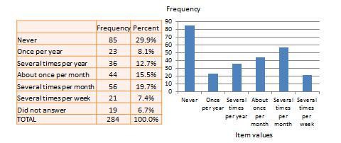
Figure 14.1. Frequency distribution of religiosity.

With very large samples where observations are independent and random, the frequency distribution tends to follow a plot that looked like a bell-shaped curve (a smoothed bar chart of the frequency distribution) similar to that shown in Figure 14.2, where most observations are clustered toward the center of the range of values, and fewer and fewer observations toward the extreme ends of the range. Such a curve is called a normal distribution.

Central tendency is an estimate of the center of a distribution of values. There are three major estimates of central tendency: mean, median, and mode. The arithmetic mean (often simply called the “mean”) is the simple average of all values in a given distribution. Consider a set of eight test scores: 15, 22, 21, 18, 36, 15, 25, 15. The arithmetic mean of these values is (15 + 20 + 21 + 20 + 36 + 15 + 25 + 15)/8 = 20.875. Other types of means include geometric mean (n th root of the product of n numbers in a distribution) and harmonic mean (the reciprocal of the arithmetic means of the reciprocal of each value in a distribution), but these means are not very popular for statistical analysis of social research data.

The second measure of central tendency, the median , is the middle value within a range of values in a distribution. This is computed by sorting all values in a distribution in increasing order and selecting the middle value. In case there are two middle values (if there is an even number of values in a distribution), the average of the two middle values represent the median. In the above example, the sorted values are: 15, 15, 15, 18, 22, 21, 25, 36. The two middle values are 18 and 22, and hence the median is (18 + 22)/2 = 20.

Lastly, the mode is the most frequently occurring value in a distribution of values. In the previous example, the most frequently occurring value is 15, which is the mode of the above set of test scores. Note that any value that is estimated from a sample, such as mean, median, mode, or any of the later estimates are called a statistic .

Dispersion refers to the way values are spread around the central tendency, for example, how tightly or how widely are the values clustered around the mean. Two common measures of dispersion are the range and standard deviation. The range is the difference between the highest and lowest values in a distribution. The range in our previous example is 36-15 = 21.

The range is particularly sensitive to the presence of outliers. For instance, if the highest value in the above distribution was 85 and the other vales remained the same, the range would be 85-15 = 70. Standard deviation , the second measure of dispersion, corrects for such outliers by using a formula that takes into account how close or how far each value from the distribution mean:

Figure 14.2. Normal distribution.

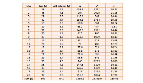
Table 14.1. Hypothetical data on age and self-esteem.

The two variables in this dataset are age (x) and self-esteem (y). Age is a ratio-scale variable, while self-esteem is an average score computed from a multi-item self-esteem scale measured using a 7-point Likert scale, ranging from “strongly disagree” to “strongly agree.” The histogram of each variable is shown on the left side of Figure 14.3. The formula for calculating bivariate correlation is:

Figure 14.3. Histogram and correlation plot of age and self-esteem.

After computing bivariate correlation, researchers are often interested in knowing whether the correlation is significant (i.e., a real one) or caused by mere chance. Answering such a question would require testing the following hypothesis:

H 0 : r = 0

H 1 : r ≠ 0

H 0 is called the null hypotheses , and H 1 is called the alternative hypothesis (sometimes, also represented as H a ). Although they may seem like two hypotheses, H 0 and H 1 actually represent a single hypothesis since they are direct opposites of each other. We are interested in testing H 1 rather than H 0 . Also note that H 1 is a non-directional hypotheses since it does not specify whether r is greater than or less than zero. Directional hypotheses will be specified as H 0 : r ≤ 0; H 1 : r > 0 (if we are testing for a positive correlation). Significance testing of directional hypothesis is done using a one-tailed t-test, while that for non-directional hypothesis is done using a two-tailed t-test.

In statistical testing, the alternative hypothesis cannot be tested directly. Rather, it is tested indirectly by rejecting the null hypotheses with a certain level of probability. Statistical testing is always probabilistic, because we are never sure if our inferences, based on sample data, apply to the population, since our sample never equals the population. The probability that a statistical inference is caused pure chance is called the p-value . The p-value is compared with the significance level (α), which represents the maximum level of risk that we are willing to take that our inference is incorrect. For most statistical analysis, α is set to 0.05. A p-value less than α=0.05 indicates that we have enough statistical evidence to reject the null hypothesis, and thereby, indirectly accept the alternative hypothesis. If p>0.05, then we do not have adequate statistical evidence to reject the null hypothesis or accept the alternative hypothesis.

The easiest way to test for the above hypothesis is to look up critical values of r from statistical tables available in any standard text book on statistics or on the Internet (most software programs also perform significance testing). The critical value of r depends on our desired significance level (α = 0.05), the degrees of freedom (df), and whether the desired test is a one-tailed or two-tailed test. The degree of freedom is the number of values that can vary freely in any calculation of a statistic. In case of correlation, the df simply equals n – 2, or for the data in Table 14.1, df is 20 – 2 = 18. There are two different statistical tables for one-tailed and two -tailed test. In the two -tailed table, the critical value of r for α = 0.05 and df = 18 is 0.44. For our computed correlation of 0.79 to be significant, it must be larger than the critical value of 0.44 or less than -0.44. Since our computed value of 0.79 is greater than 0.44, we conclude that there is a significant correlation between age and self-esteem in our data set, or in other words, the odds are less than 5% that this correlation is a chance occurrence. Therefore, we can reject the null hypotheses that r ≤ 0, which is an indirect way of saying that the alternative hypothesis r > 0 is probably correct.

Most research studies involve more than two variables. If there are n variables, then we will have a total of n*(n-1)/2 possible correlations between these n variables. Such correlations are easily computed using a software program like SPSS, rather than manually using the formula for correlation (as we did in Table 14.1), and represented using a correlation matrix, as shown in Table 14.2. A correlation matrix is a matrix that lists the variable names along the first row and the first column, and depicts bivariate correlations between pairs of variables in the appropriate cell in the matrix. The values along the principal diagonal (from the top left to the bottom right corner) of this matrix are always 1, because any variable is always perfectly correlated with itself. Further, since correlations are non-directional, the correlation between variables V1 and V2 is the same as that between V2 and V1. Hence, the lower triangular matrix (values below the principal diagonal) is a mirror reflection of the upper triangular matrix (values above the principal diagonal), and therefore, we often list only the lower triangular matrix for simplicity. If the correlations involve variables measured using interval scales, then this specific type of correlations are called Pearson product moment correlations .

Another useful way of presenting bivariate data is cross-tabulation (often abbreviated to cross-tab, and sometimes called more formally as a contingency table). A cross-tab is a table that describes the frequency (or percentage) of all combinations of two or more nominal or categorical variables. As an example, let us assume that we have the following observations of gender and grade for a sample of 20 students, as shown in Figure 14.3. Gender is a nominal variable (male/female or M/F), and grade is a categorical variable with three levels (A, B, and C). A simple cross-tabulation of the data may display the joint distribution of gender and grades (i.e., how many students of each gender are in each grade category, as a raw frequency count or as a percentage) in a 2 x 3 matrix. This matrix will help us see if A, B, and C grades are equally distributed across male and female students. The cross-tab data in Table 14.3 shows that the distribution of A grades is biased heavily toward female students: in a sample of 10 male and 10 female students, five female students received the A grade compared to only one male students. In contrast, the distribution of C grades is biased toward male students: three male students received a C grade, compared to only one female student. However, the distribution of B grades was somewhat uniform, with six male students and five female students. The last row and the last column of this table are called marginal totals because they indicate the totals across each category and displayed along the margins of the table.

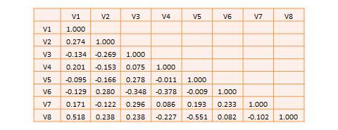
Table 14.2. A hypothetical correlation matrix for eight variables.

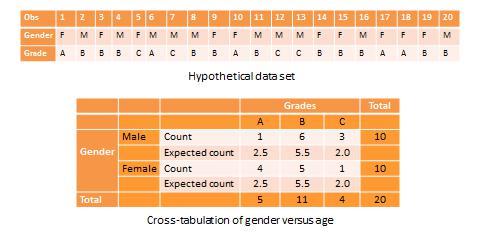
Table 14.3. Example of cross-tab analysis.

Although we can see a distinct pattern of grade distribution between male and female students in Table 14.3, is this pattern real or “statistically significant”? In other words, do the above frequency counts differ from that that may be expected from pure chance? To answer this question, we should compute the expected count of observation in each cell of the 2 x 3 cross-tab matrix. This is done by multiplying the marginal column total and the marginal row total for each cell and dividing it by the total number of observations. For example, for the male/A grade cell, expected count = 5 * 10 / 20 = 2.5. In other words, we were expecting 2.5 male students to receive an A grade, but in reality, only one student received the A grade. Whether this difference between expected and actual count is significant can be tested using a chi-square test . The chi-square statistic can be computed as the average difference between observed and expected counts across all cells. We can then compare this number to the critical value associated with a desired probability level (p < 0.05) and the degrees of freedom, which is simply (m-1)*(n-1), where m and n are the number of rows and columns respectively. In this example, df = (2 – 1) * (3 – 1) = 2. From standard chi-square tables in any statistics book, the critical chi-square value for p=0.05 and df=2 is 5.99. The computed chi -square value, based on our observed data, is 1.00, which is less than the critical value. Hence, we must conclude that the observed grade pattern is not statistically different from the pattern that can be expected by pure chance.

• Social Science Research: Principles, Methods, and Practices. Authored by : Anol Bhattacherjee. Provided by : University of South Florida. Located at : http://scholarcommons.usf.edu/oa_textbooks/3/ . License : CC BY-NC-SA: Attribution-NonCommercial-ShareAlike

Root out friction in every digital experience, super-charge conversion rates, and optimize digital self-service

Uncover insights from any interaction, deliver AI-powered agent coaching, and reduce cost to serve

Increase revenue and loyalty with real-time insights and recommendations delivered to teams on the ground

Know how your people feel and empower managers to improve employee engagement, productivity, and retention

Take action in the moments that matter most along the employee journey and drive bottom line growth

Whatever they’re are saying, wherever they’re saying it, know exactly what’s going on with your people

Get faster, richer insights with qual and quant tools that make powerful market research available to everyone

Run concept tests, pricing studies, prototyping + more with fast, powerful studies designed by UX research experts

Track your brand performance 24/7 and act quickly to respond to opportunities and challenges in your market

Explore the platform powering Experience Management

• Free Account
• For Digital
• For Customer Care
• For Human Resources
• For Researchers
• Financial Services
• All Industries

Popular Use Cases

• Customer Experience
• Employee Experience
• Net Promoter Score
• Voice of Customer
• Customer Success Hub
• Product Documentation
• Training & Certification
• XM Institute
• Popular Resources
• Customer Stories
• Artificial Intelligence

Market Research

• Partnerships
• Marketplace

The annual gathering of the experience leaders at the world’s iconic brands building breakthrough business results, live in Salt Lake City.

• English/AU & NZ
• Español/Europa
• Español/América Latina
• Português Brasileiro
• REQUEST DEMO
• Experience Management
• Descriptive Statistics

Try Qualtrics for free

Descriptive statistics in research: a critical component of data analysis.

15 min read With any data, the object is to describe the population at large, but what does that mean and what processes, methods and measures are used to uncover insights from that data? In this short guide, we explore descriptive statistics and how it’s applied to research.

What do we mean by descriptive statistics?

With any kind of data, the main objective is to describe a population at large — and using descriptive statistics, researchers can quantify and describe the basic characteristics of a given data set.

For example, researchers can condense large data sets, which may contain thousands of individual data points or observations, into a series of statistics that provide useful information on the population of interest. We call this process “describing data”.

In the process of producing summaries of the sample, we use measures like mean, median, variance, graphs, charts, frequencies, histograms, box and whisker plots, and percentages. For datasets with just one variable, we use univariate descriptive statistics. For datasets with multiple variables, we use bivariate correlation and multivariate descriptive statistics.

Want to find out the definitions?

Univariate descriptive statistics: this is when you want to describe data with only one characteristic or attribute

Bivariate correlation: this is when you simultaneously analyze (compare) two variables to see if there is a relationship between them

Multivariate descriptive statistics: this is a subdivision of statistics encompassing the simultaneous observation and analysis of more than one outcome variable

Then, after describing and summarizing the data, as well as using simple graphical analyses, we can start to draw meaningful insights from it to help guide specific strategies. It’s also important to note that descriptive statistics can employ and use both quantitative and qualitative research .

Describing data is undoubtedly the most critical first step in research as it enables the subsequent organization, simplification and summarization of information — and every survey question and population has summary statistics. Let’s take a look at a few examples.

Examples of descriptive statistics

Consider for a moment a number used to summarize how well a striker is performing in football — goals scored per game. This number is simply the number of shots taken against how many of those shots hit the back of the net (reported to three significant digits). If a striker is scoring 0.333, that’s one goal for every three shots. If they’re scoring one in four, that’s 0.250.

A classic example is a student’s grade point average (GPA). This single number describes the general performance of a student across a range of course experiences and classes. It doesn’t tell us anything about the difficulty of the courses the student is taking, or what those courses are, but it does provide a summary that enables a degree of comparison with people or other units of data.

Ultimately, descriptive statistics make it incredibly easy for people to understand complex (or data intensive) quantitative or qualitative insights across large data sets.

Take your research to the next level with XM for Strategy & Research

Types of descriptive statistics

To quantitatively summarize the characteristics of raw, ungrouped data, we use the following types of descriptive statistics:

• Measures of Central Tendency ,
• Measures of Dispersion and
• Measures of Frequency Distribution.

Following the application of any of these approaches, the raw data then becomes ‘grouped’ data that’s logically organized and easy to understand. To visually represent the data, we then use graphs, charts, tables etc.

Let’s look at the different types of measurement and the statistical methods that belong to each:

Measures of Central Tendency are used to describe data by determining a single representative of central value. For example, the mean, median or mode.

Measures of Dispersion are used to determine how spread out a data distribution is with respect to the central value, e.g. the mean, median or mode. For example, while central tendency gives the person the average or central value, it doesn’t describe how the data is distributed within the set.

Measures of Frequency Distribution are used to describe the occurrence of data within the data set (count).

The methods of each measure are summarized in the table below:

Mean: The most popular and well-known measure of central tendency. The mean is equal to the sum of all the values in the data set divided by the number of values in the data set.

Median: The median is the middle score for a set of data that has been arranged in order of magnitude. If you have an even number of data, e.g. 10 data points, take the two middle scores and average the result.

Mode: The mode is the most frequently occurring observation in the data set.  

Range: The difference between the highest and lowest value.

Standard deviation: Standard deviation measures the dispersion of a data set relative to its mean and is calculated as the square root of the variance.

Quartile deviation : Quartile deviation measures the deviation in the middle of the data.

Variance: Variance measures the variability from the average of mean.

Absolute deviation: The absolute deviation of a dataset is the average distance between each data point and the mean.

Count: How often each value occurs.

Scope of descriptive statistics in research

Descriptive statistics (or analysis) is considered more vast than other quantitative and qualitative methods as it provides a much broader picture of an event, phenomenon or population.

But that’s not all: it can use any number of variables, and as it collects data and describes it as it is, it’s also far more representative of the world as it exists.

However, it’s also important to consider that descriptive analyses lay the foundation for further methods of study. By summarizing and condensing the data into easily understandable segments, researchers can further analyze the data to uncover new variables or hypotheses.

Mostly, this practice is all about the ease of data visualization. With data presented in a meaningful way, researchers have a simplified interpretation of the data set in question. That said, while descriptive statistics helps to summarize information, it only provides a general view of the variables in question.

It is, therefore, up to the researchers to probe further and use other methods of analysis to discover deeper insights.

Things you can do with descriptive statistics

Define subject characteristics

If a marketing team wanted to build out accurate buyer personas for specific products and industry verticals, they could use descriptive analyses on customer datasets (procured via a survey) to identify consistent traits and behaviors.

They could then ‘describe’ the data to build a clear picture and understanding of who their buyers are, including things like preferences, business challenges, income and so on.

Measure data trends

Let’s say you wanted to assess propensity to buy over several months or years for a specific target market and product. With descriptive statistics, you could quickly summarize the data and extract the precise data points you need to understand the trends in product purchase behavior.

Compare events, populations or phenomena

How do different demographics respond to certain variables? For example, you might want to run a customer study to see how buyers in different job functions respond to new product features or price changes. Are all groups as enthusiastic about the new features and likely to buy? Or do they have reservations? This kind of data will help inform your overall product strategy and potentially how you tier solutions.

Validate existing conditions

When you have a belief or hypothesis but need to prove it, you can use descriptive techniques to ascertain underlying patterns or assumptions.

Form new hypotheses

With the data presented and surmised in a way that everyone can understand (and infer connections from), you can delve deeper into specific data points to uncover deeper and more meaningful insights — or run more comprehensive research.

Guiding your survey design to improve the data collected

To use your surveys as an effective tool for customer engagement and understanding, every survey goal and item should answer one simple, yet highly important question:

What am I really asking?

It might seem trivial, but by having this question frame survey research, it becomes significantly easier for researchers to develop the right questions that uncover useful, meaningful and actionable insights.

Planning becomes easier, questions clearer and perspective far wider and yet nuanced.

Hypothesize – what’s the problem that you’re trying to solve? Far too often, organizations collect data without understanding what they’re asking, and why they’re asking it.

Finally, focus on the end result. What kind of data do you need to answer your question? Also, are you asking a quantitative or qualitative question? Here are a few things to consider:

• Clear questions are clear for everyone. It takes time to make a concept clear
• Ask about measurable, evident and noticeable activities or behaviors.
• Make rating scales easy. Avoid long lists, confusing scales or “don’t know” or “not applicable” options.
• Ensure your survey makes sense and flows well. Reduce the cognitive load on respondents by making it easy for them to complete the survey.
• Read your questions aloud to see how they sound.
• Pretest by asking a few uninvolved individuals to answer.

Furthermore…

As well as understanding what you’re really asking, there are several other considerations for your data:

Keep it random

How you select your sample is what makes your research replicable and meaningful. Having a truly random sample helps prevent bias, increasingly the quality of evidence you find.

Plan for and avoid sample error

Before starting your research project, have a clear plan for avoiding sample error. Use larger sample sizes, and apply random sampling to minimize the potential for bias.

Don’t over sample

Remember, you can sample 500 respondents selected randomly from a population and they will closely reflect the actual population 95% of the time.

Think about the mode

Match your survey methods to the sample you select. For example, how do your current customers prefer communicating? Do they have any shared characteristics or preferences? A mixed-method approach is critical if you want to drive action across different customer segments.

Use a survey tool that supports you with the whole process

Surveys created using a survey research software can support researchers in a number of ways:

• Employee satisfaction survey template
• Employee exit survey template
• Customer satisfaction (CSAT) survey template
• Ad testing survey template
• Brand awareness survey template
• Product pricing survey template
• Product research survey template
• Employee engagement survey template
• Customer service survey template
• NPS survey template
• Product package testing survey template
• Product features prioritization survey template

These considerations have been included in Qualtrics’ survey software , which summarizes and creates visualizations of data, making it easy to access insights, measure trends, and examine results without complexity or jumping between systems.

Uncover your next breakthrough idea with Stats iQ™

What makes Qualtrics so different from other survey providers is that it is built in consultation with trained research professionals and includes high-tech statistical software like Qualtrics Stats iQ .

With just a click, the software can run specific analyses or automate statistical testing and data visualization. Testing parameters are automatically chosen based on how your data is structured (e.g. categorical data will run a statistical test like Chi-squared), and the results are translated into plain language that anyone can understand and put into action.

Get more meaningful insights from your data

Stats iQ includes a variety of statistical analyses, including: describe, relate, regression, cluster, factor, TURF, and pivot tables — all in one place!

Confidently analyze complex data

Built-in artificial intelligence and advanced algorithms automatically choose and apply the right statistical analyses and return the insights in plain english so everyone can take action.

Integrate existing statistical workflows

For more experienced stats users, built-in R code templates allow you to run even more sophisticated analyses by adding R code snippets directly in your survey analysis.

Advanced statistical analysis methods available in Stats iQ

Regression analysis – Measures the degree of influence of independent variables on a dependent variable (the relationship between two or multiple variables).

Analysis of Variance (ANOVA) test – Commonly used with a regression study to find out what effect independent variables have on the dependent variable. It can compare multiple groups simultaneously to see if there is a relationship between them.

Conjoint analysis – Asks people to make trade-offs when making decisions, then analyses the results to give the most popular outcome. Helps you understand why people make the complex choices they do.

T-Test – Helps you compare whether two data groups have different mean values and allows the user to interpret whether differences are meaningful or merely coincidental.

Crosstab analysis – Used in quantitative market research to analyze categorical data – that is, variables that are different and mutually exclusive, and allows you to compare the relationship between two variables in contingency tables.

Go from insights to action

Now that you have a better understanding of descriptive statistics in research and how you can leverage statistical analysis methods correctly, now’s the time to utilize a tool that can take your research and subsequent analysis to the next level.

Try out a Qualtrics survey software demo so you can see how it can take you through descriptive research and further research projects from start to finish.

Take your research to the next level with XM for Strategy & Research

Related resources

Market intelligence 10 min read, marketing insights 11 min read, ethnographic research 11 min read, qualitative vs quantitative research 13 min read, qualitative research questions 11 min read, qualitative research design 12 min read, primary vs secondary research 14 min read, request demo.

Ready to learn more about Qualtrics?

• Calculators
• Descriptive Statistics
• Merchandise
• Which Statistics Test?

Tools for Descriptive Statistics

• Scatter Plot Chart Maker, with Line of Best Fit (Offsite)
• Mean, Median and Mode Calculator
• Variance Calculator
• Standard Deviation Calculator
• Coefficient of Variation Calculator
• Percentile Calculator
• Interquartile Range Calculator
• Pooled Variance Calculator
• Skewness and Kurtosis Calculator
• Sum of Squares Calculator
• Easy Histogram Maker
• Frequency Distribution Calculator
• Histogram: What are they? How do you make one?
• Easy Frequency Polygon Maker
• Easy Bar Chart Creator

Effective Use of Statistics in Research – Methods and Tools for Data Analysis

Remember that impending feeling you get when you are asked to analyze your data! Now that you have all the required raw data, you need to statistically prove your hypothesis. Representing your numerical data as part of statistics in research will also help in breaking the stereotype of being a biology student who can’t do math.

Statistical methods are essential for scientific research. In fact, statistical methods dominate the scientific research as they include planning, designing, collecting data, analyzing, drawing meaningful interpretation and reporting of research findings. Furthermore, the results acquired from research project are meaningless raw data unless analyzed with statistical tools. Therefore, determining statistics in research is of utmost necessity to justify research findings. In this article, we will discuss how using statistical methods for biology could help draw meaningful conclusion to analyze biological studies.

Table of Contents

Role of Statistics in Biological Research

Statistics is a branch of science that deals with collection, organization and analysis of data from the sample to the whole population. Moreover, it aids in designing a study more meticulously and also give a logical reasoning in concluding the hypothesis. Furthermore, biology study focuses on study of living organisms and their complex living pathways, which are very dynamic and cannot be explained with logical reasoning. However, statistics is more complex a field of study that defines and explains study patterns based on the sample sizes used. To be precise, statistics provides a trend in the conducted study.

Biological researchers often disregard the use of statistics in their research planning, and mainly use statistical tools at the end of their experiment. Therefore, giving rise to a complicated set of results which are not easily analyzed from statistical tools in research. Statistics in research can help a researcher approach the study in a stepwise manner, wherein the statistical analysis in research follows –

1. Establishing a Sample Size

Usually, a biological experiment starts with choosing samples and selecting the right number of repetitive experiments. Statistics in research deals with basics in statistics that provides statistical randomness and law of using large samples. Statistics teaches how choosing a sample size from a random large pool of sample helps extrapolate statistical findings and reduce experimental bias and errors.

2. Testing of Hypothesis

When conducting a statistical study with large sample pool, biological researchers must make sure that a conclusion is statistically significant. To achieve this, a researcher must create a hypothesis before examining the distribution of data. Furthermore, statistics in research helps interpret the data clustered near the mean of distributed data or spread across the distribution. These trends help analyze the sample and signify the hypothesis.

3. Data Interpretation Through Analysis

When dealing with large data, statistics in research assist in data analysis. This helps researchers to draw an effective conclusion from their experiment and observations. Concluding the study manually or from visual observation may give erroneous results; therefore, thorough statistical analysis will take into consideration all the other statistical measures and variance in the sample to provide a detailed interpretation of the data. Therefore, researchers produce a detailed and important data to support the conclusion.

Types of Statistical Research Methods That Aid in Data Analysis

Statistical analysis is the process of analyzing samples of data into patterns or trends that help researchers anticipate situations and make appropriate research conclusions. Based on the type of data, statistical analyses are of the following type:

1. Descriptive Analysis

The descriptive statistical analysis allows organizing and summarizing the large data into graphs and tables . Descriptive analysis involves various processes such as tabulation, measure of central tendency, measure of dispersion or variance, skewness measurements etc.

2. Inferential Analysis

The inferential statistical analysis allows to extrapolate the data acquired from a small sample size to the complete population. This analysis helps draw conclusions and make decisions about the whole population on the basis of sample data. It is a highly recommended statistical method for research projects that work with smaller sample size and meaning to extrapolate conclusion for large population.

3. Predictive Analysis

Predictive analysis is used to make a prediction of future events. This analysis is approached by marketing companies, insurance organizations, online service providers, data-driven marketing, and financial corporations.

4. Prescriptive Analysis

Prescriptive analysis examines data to find out what can be done next. It is widely used in business analysis for finding out the best possible outcome for a situation. It is nearly related to descriptive and predictive analysis. However, prescriptive analysis deals with giving appropriate suggestions among the available preferences.

5. Exploratory Data Analysis

EDA is generally the first step of the data analysis process that is conducted before performing any other statistical analysis technique. It completely focuses on analyzing patterns in the data to recognize potential relationships. EDA is used to discover unknown associations within data, inspect missing data from collected data and obtain maximum insights.

6. Causal Analysis

Causal analysis assists in understanding and determining the reasons behind “why” things happen in a certain way, as they appear. This analysis helps identify root cause of failures or simply find the basic reason why something could happen. For example, causal analysis is used to understand what will happen to the provided variable if another variable changes.

7. Mechanistic Analysis

This is a least common type of statistical analysis. The mechanistic analysis is used in the process of big data analytics and biological science. It uses the concept of understanding individual changes in variables that cause changes in other variables correspondingly while excluding external influences.

Important Statistical Tools In Research

Researchers in the biological field find statistical analysis in research as the scariest aspect of completing research. However, statistical tools in research can help researchers understand what to do with data and how to interpret the results, making this process as easy as possible.

1. Statistical Package for Social Science (SPSS)

It is a widely used software package for human behavior research. SPSS can compile descriptive statistics, as well as graphical depictions of result. Moreover, it includes the option to create scripts that automate analysis or carry out more advanced statistical processing.

2. R Foundation for Statistical Computing

This software package is used among human behavior research and other fields. R is a powerful tool and has a steep learning curve. However, it requires a certain level of coding. Furthermore, it comes with an active community that is engaged in building and enhancing the software and the associated plugins.

3. MATLAB (The Mathworks)

It is an analytical platform and a programming language. Researchers and engineers use this software and create their own code and help answer their research question. While MatLab can be a difficult tool to use for novices, it offers flexibility in terms of what the researcher needs.

4. Microsoft Excel

Not the best solution for statistical analysis in research, but MS Excel offers wide variety of tools for data visualization and simple statistics. It is easy to generate summary and customizable graphs and figures. MS Excel is the most accessible option for those wanting to start with statistics.

5. Statistical Analysis Software (SAS)

It is a statistical platform used in business, healthcare, and human behavior research alike. It can carry out advanced analyzes and produce publication-worthy figures, tables and charts .

6. GraphPad Prism

It is a premium software that is primarily used among biology researchers. But, it offers a range of variety to be used in various other fields. Similar to SPSS, GraphPad gives scripting option to automate analyses to carry out complex statistical calculations.

This software offers basic as well as advanced statistical tools for data analysis. However, similar to GraphPad and SPSS, minitab needs command over coding and can offer automated analyses.

Use of Statistical Tools In Research and Data Analysis

Statistical tools manage the large data. Many biological studies use large data to analyze the trends and patterns in studies. Therefore, using statistical tools becomes essential, as they manage the large data sets, making data processing more convenient.

Following these steps will help biological researchers to showcase the statistics in research in detail, and develop accurate hypothesis and use correct tools for it.

There are a range of statistical tools in research which can help researchers manage their research data and improve the outcome of their research by better interpretation of data. You could use statistics in research by understanding the research question, knowledge of statistics and your personal experience in coding.

Have you faced challenges while using statistics in research? How did you manage it? Did you use any of the statistical tools to help you with your research data? Do write to us or comment below!

Frequently Asked Questions

Statistics in research can help a researcher approach the study in a stepwise manner: 1. Establishing a sample size 2. Testing of hypothesis 3. Data interpretation through analysis

Statistical methods are essential for scientific research. In fact, statistical methods dominate the scientific research as they include planning, designing, collecting data, analyzing, drawing meaningful interpretation and reporting of research findings. Furthermore, the results acquired from research project are meaningless raw data unless analyzed with statistical tools. Therefore, determining statistics in research is of utmost necessity to justify research findings.

Statistical tools in research can help researchers understand what to do with data and how to interpret the results, making this process as easy as possible. They can manage large data sets, making data processing more convenient. A great number of tools are available to carry out statistical analysis of data like SPSS, SAS (Statistical Analysis Software), and Minitab.

nice article to read

Holistic but delineating. A very good read.

Rate this article Cancel Reply

Your email address will not be published.

Enago Academy's Most Popular Articles

• Promoting Research
• Thought Leadership
• Trending Now

How Enago Academy Contributes to Sustainable Development Goals (SDGs) Through Empowering Researchers

The United Nations Sustainable Development Goals (SDGs) are a universal call to action to end…

• Reporting Research

Research Interviews: An effective and insightful way of data collection

Research interviews play a pivotal role in collecting data for various academic, scientific, and professional…

Planning Your Data Collection: Designing methods for effective research

Planning your research is very important to obtain desirable results. In research, the relevance of…

• Language & Grammar

Best Plagiarism Checker Tool for Researchers — Top 4 to choose from!

While common writing issues like language enhancement, punctuation errors, grammatical errors, etc. can be dealt…

• Industry News
• Publishing News

2022 in a Nutshell — Reminiscing the year when opportunities were seized and feats were achieved!

It’s beginning to look a lot like success! Some of the greatest opportunities to research…

2022 in a Nutshell — Reminiscing the year when opportunities were seized and feats…

Sign-up to read more

Subscribe for free to get unrestricted access to all our resources on research writing and academic publishing including:

• 2000+ blog articles
• 50+ Webinars
• 10+ Expert podcasts
• 50+ Infographics
• 10+ Checklists
• Research Guides

We hate spam too. We promise to protect your privacy and never spam you.

I am looking for Editing/ Proofreading services for my manuscript Tentative date of next journal submission:

As a researcher, what do you consider most when choosing an image manipulation detector?

An official website of the United States government

The .gov means it's official. Federal government websites often end in .gov or .mil. Before sharing sensitive information, make sure you're on a federal government site.

The site is secure. The https:// ensures that you are connecting to the official website and that any information you provide is encrypted and transmitted securely.

• Publications
• Account settings
• Browse Titles

NCBI Bookshelf. A service of the National Library of Medicine, National Institutes of Health.

StatPearls [Internet]. Treasure Island (FL): StatPearls Publishing; 2024 Jan-.

StatPearls [Internet].

Exploratory data analysis: frequencies, descriptive statistics, histograms, and boxplots.

Jacob Shreffler ; Martin R. Huecker .

Affiliations

Last Update: November 3, 2023 .

• Definition/Introduction

Researchers must utilize exploratory data techniques to present findings to a target audience and create appropriate graphs and figures. Researchers can determine if outliers exist, data are missing, and statistical assumptions will be upheld by understanding data. Additionally, it is essential to comprehend these data when describing them in conclusions of a paper, in a meeting with colleagues invested in the findings, or while reading others’ work.

• Issues of Concern

This comprehension begins with exploring these data through the outputs discussed in this article. Individuals who do not conduct research must still comprehend new studies, and knowledge of fundamentals in analyzing data and interpretation of histograms and boxplots facilitates the ability to appraise recent publications accurately. Without this familiarity, decisions could be implemented based on inaccurate delivery or interpretation of medical studies.

Frequencies and Descriptive Statistics

Effective presentation of study results, in presentation or manuscript form, typically starts with frequencies and descriptive statistics (ie, mean, medians, standard deviations). One can get a better sense of the variables by examining these data to determine whether a balanced and sufficient research design exists. Frequencies also inform on missing data and give a sense of outliers (will be discussed below).

Luckily, software programs are available to conduct exploratory data analysis. For this chapter, we will be examining the following research question.

RQ: Are there differences in drug life (length of effect) for Drug 23 based on the administration site?

A more precise hypothesis could be: Is drug 23 longer-lasting when administered via site A compared to site B?

To address this research question, exploratory data analysis is conducted. First, it is essential to start with the frequencies of the variables. To keep things simple, only variables of minutes (drug life effect) and administration site (A vs B) are included. See Image. Figure 1 for outputs for frequencies.

Figure 1 shows that the administration site appears to be a balanced design with 50 individuals in each group. The excerpt for minutes frequencies is the bottom portion of Figure 1 and shows how many cases fell into each time frame with the cumulative percent on the right-hand side. In examining Figure 1, one suspiciously low measurement (135) was observed, considering time variables. If a data point seems inaccurate, a researcher should find this case and confirm if this was an entry error. For the sake of this review, the authors state that this was an entry error and should have been entered 535 and not 135. Had the analysis occurred without checking this, the data analysis, results, and conclusions would have been invalid. When finding any entry errors and determining how groups are balanced, potential missing data is explored. If not responsibly evaluated, missing values can nullify results.  

After replacing the incorrect 135 with 535, descriptive statistics, including the mean, median, mode, minimum/maximum scores, and standard deviation were examined. Output for the research example for the variable of minutes can be seen in Figure 2. Observe each variable to ensure that the mean seems reasonable and that the minimum and maximum are within an appropriate range based on medical competence or an available codebook. One assumption common in statistical analyses is a normal distribution. Image . Figure 2 shows that the mode differs from the mean and the median. We have visualization tools such as histograms to examine these scores for normality and outliers before making decisions.

Histograms are useful in assessing normality, as many statistical tests (eg, ANOVA and regression) assume the data have a normal distribution. When data deviate from a normal distribution, it is quantified using skewness and kurtosis. [1]  Skewness occurs when one tail of the curve is longer. If the tail is lengthier on the left side of the curve (more cases on the higher values), this would be negatively skewed, whereas if the tail is longer on the right side, it would be positively skewed. Kurtosis is another facet of normality. Positive kurtosis occurs when the center has many values falling in the middle, whereas negative kurtosis occurs when there are very heavy tails. [2]

Additionally, histograms reveal outliers: data points either entered incorrectly or truly very different from the rest of the sample. When there are outliers, one must determine accuracy based on random chance or the error in the experiment and provide strong justification if the decision is to exclude them. [3]  Outliers require attention to ensure the data analysis accurately reflects the majority of the data and is not influenced by extreme values; cleaning these outliers can result in better quality decision-making in clinical practice. [4]  A common approach to determining if a variable is approximately normally distributed is converting values to z scores and determining if any scores are less than -3 or greater than 3. For a normal distribution, about 99% of scores should lie within three standard deviations of the mean. [5]  Importantly, one should not automatically throw out any values outside of this range but consider it in corroboration with the other factors aforementioned. Outliers are relatively common, so when these are prevalent, one must assess the risks and benefits of exclusion. [6]

Image . Figure 3 provides examples of histograms. In Figure 3A, 2 possible outliers causing kurtosis are observed. If values within 3 standard deviations are used, the result in Figure 3B are observed. This histogram appears much closer to an approximately normal distribution with the kurtosis being treated. Remember, all evidence should be considered before eliminating outliers. When reporting outliers in scientific paper outputs, account for the number of outliers excluded and justify why they were excluded.

Boxplots can examine for outliers, assess the range of data, and show differences among groups. Boxplots provide a visual representation of ranges and medians, illustrating differences amongst groups, and are useful in various outlets, including evidence-based medicine. [7]  Boxplots provide a picture of data distribution when there are numerous values, and all values cannot be displayed (ie, a scatterplot). [8]  Figure 4 illustrates the differences between drug site administration and the length of drug life from the above example.

Image . Figure 4 shows differences with potential clinical impact. Had any outliers existed (data from the histogram were cleaned), they would appear outside the line endpoint. The red boxes represent the middle 50% of scores. The lines within each red box represent the median number of minutes within each administration site. The horizontal lines at the top and bottom of each line connected to the red box represent the 25th and 75th percentiles. In examining the difference boxplots, an overlap in minutes between 2 administration sites were observed: the approximate top 25 percent from site B had the same time noted as the bottom 25 percent at site A. Site B had a median minute amount under 525, whereas administration site A had a length greater than 550. If there were no differences in adverse reactions at site A, analysis of this figure provides evidence that healthcare providers should administer the drug via site A. Researchers could follow by testing a third administration site, site C. Image . Figure 5 shows what would happen if site C led to a longer drug life compared to site A.

Figure 5 displays the same site A data as Figure 4, but something looks different. The significant variance at site C makes site A’s variance appear smaller. In order words, patients who were administered the drug via site C had a larger range of scores. Thus, some patients experience a longer half-life when the drug is administered via site C than the median of site A; however, the broad range (lack of accuracy) and lower median should be the focus. The precision of minutes is much more compacted in site A. Therefore, the median is higher, and the range is more precise. One may conclude that this makes site A a more desirable site.

• Clinical Significance

Ultimately, by understanding basic exploratory data methods, medical researchers and consumers of research can make quality and data-informed decisions. These data-informed decisions will result in the ability to appraise the clinical significance of research outputs. By overlooking these fundamentals in statistics, critical errors in judgment can occur.

• Nursing, Allied Health, and Interprofessional Team Interventions

All interprofessional healthcare team members need to be at least familiar with, if not well-versed in, these statistical analyses so they can read and interpret study data and apply the data implications in their everyday practice. This approach allows all practitioners to remain abreast of the latest developments and provides valuable data for evidence-based medicine, ultimately leading to improved patient outcomes.

• Review Questions
• Access free multiple choice questions on this topic.
• Comment on this article.

Exploratory Data Analysis Figure 1 Contributed by Martin Huecker, MD and Jacob Shreffler, PhD

Exploratory Data Analysis Figure 2 Contributed by Martin Huecker, MD and Jacob Shreffler, PhD

Exploratory Data Analysis Figure 3 Contributed by Martin Huecker, MD and Jacob Shreffler, PhD

Exploratory Data Analysis Figure 4 Contributed by Martin Huecker, MD and Jacob Shreffler, PhD

Exploratory Data Analysis Figure 5 Contributed by Martin Huecker, MD and Jacob Shreffler, PhD

Disclosure: Jacob Shreffler declares no relevant financial relationships with ineligible companies.

Disclosure: Martin Huecker declares no relevant financial relationships with ineligible companies.

This book is distributed under the terms of the Creative Commons Attribution-NonCommercial-NoDerivatives 4.0 International (CC BY-NC-ND 4.0) ( http://creativecommons.org/licenses/by-nc-nd/4.0/ ), which permits others to distribute the work, provided that the article is not altered or used commercially. You are not required to obtain permission to distribute this article, provided that you credit the author and journal.

• Cite this Page Shreffler J, Huecker MR. Exploratory Data Analysis: Frequencies, Descriptive Statistics, Histograms, and Boxplots. [Updated 2023 Nov 3]. In: StatPearls [Internet]. Treasure Island (FL): StatPearls Publishing; 2024 Jan-.

In this Page

Bulk download.

• Bulk download StatPearls data from FTP

Related information

• PMC PubMed Central citations
• PubMed Links to PubMed

Similar articles in PubMed

• Contour boxplots: a method for characterizing uncertainty in feature sets from simulation ensembles. [IEEE Trans Vis Comput Graph. 2...] Contour boxplots: a method for characterizing uncertainty in feature sets from simulation ensembles. Whitaker RT, Mirzargar M, Kirby RM. IEEE Trans Vis Comput Graph. 2013 Dec; 19(12):2713-22.
• Review Univariate Outliers: A Conceptual Overview for the Nurse Researcher. [Can J Nurs Res. 2019] Review Univariate Outliers: A Conceptual Overview for the Nurse Researcher. Mowbray FI, Fox-Wasylyshyn SM, El-Masri MM. Can J Nurs Res. 2019 Mar; 51(1):31-37. Epub 2018 Jul 3.
• Qualitative Study. [StatPearls. 2024] Qualitative Study. Tenny S, Brannan JM, Brannan GD. StatPearls. 2024 Jan
• [Descriptive statistics]. [Rev Alerg Mex. 2016] [Descriptive statistics]. Rendón-Macías ME, Villasís-Keever MÁ, Miranda-Novales MG. Rev Alerg Mex. 2016 Oct-Dec; 63(4):397-407.
• Review Graphics and statistics for cardiology: comparing categorical and continuous variables. [Heart. 2016] Review Graphics and statistics for cardiology: comparing categorical and continuous variables. Rice K, Lumley T. Heart. 2016 Mar; 102(5):349-55. Epub 2016 Jan 27.

Recent Activity

• Exploratory Data Analysis: Frequencies, Descriptive Statistics, Histograms, and ... Exploratory Data Analysis: Frequencies, Descriptive Statistics, Histograms, and Boxplots - StatPearls

Your browsing activity is empty.

Activity recording is turned off.

Turn recording back on

Connect with NLM

National Library of Medicine 8600 Rockville Pike Bethesda, MD 20894

Web Policies FOIA HHS Vulnerability Disclosure

Help Accessibility Careers

Top 9 Statistical Tools Used in Research

Well-designed research requires a well-chosen study sample and a suitable statistical test selection . To plan an epidemiological study or a clinical trial, you’ll need a solid understanding of the data . Improper inferences from it could lead to false conclusions and  unethical behavior . And given the ocean of data available nowadays, it’s often a daunting task for researchers to gauge its credibility and do statistical analysis on it.

With that said, thanks to all the statistical tools available in the market that help researchers make such studies much more manageable.  Statistical tools are   extensively used in academic and research sectors  to study human, animal, and material behaviors and reactions.

Statistical tools  aid in the interpretation and use of data. They can be used to evaluate and comprehend any form of data. Some statistical tools can help you see trends, forecast future sales, and create links between causes and effects. When you’re unsure where to go with your study, other tools can assist you in navigating through enormous amounts of data.

In this article, we will  discuss some  of the best statistical tools and their key features . So, let’s start without any further ado.

What is Statistics? And its Importance in Research

Statistics is the study of collecting, arranging, and interpreting data from samples and inferring it to the total population.  Also  known  as the “Science of Data,” it allows us to derive conclusions from a data set. It may also assist people in all industries in answering research or business queries and forecast outcomes, such as what show you should watch next on your favorite video app.

Statistical Tools Used in Research

Researchers often cannot discern a simple truth from a set of data. They can only draw conclusions from data after statistical analysis. On the other hand, creating a statistical analysis is a difficult task. This is when statistical tools come into play. Researchers can use statistical tools to back up their claims, make sense of a vast set of data, graphically show complex data, or help clarify many things in a short period. 

Let’s go through  the top 9 best statistical tools used in research  below:

SPSS (Statistical Package for the Social Sciences)  is a collection of software tools compiled as a single package. This program’s primary function is to analyze scientific data in social science. This information can be utilized for market research, surveys, and data mining, among other things. It is mainly used in the following areas like marketing, healthcare, educational research, etc.

SPSS first stores and organizes the data, then compile the data set to generate appropriate output. SPSS is intended to work with a wide range of variable data formats.

Some of the  highlights of SPSS :

• It gives you greater tools for analyzing and comprehending your data. With SPSS’s excellent interface, you can easily handle complex commercial and research challenges.
•  It assists you in making accurate and high-quality decisions.
• It also comes with a variety of deployment options for managing your software.
• You may also use a point-and-click interface to produce unique visualizations and reports. To start using SPSS, you don’t need prior coding skills.
•  It provides the best views of missing data patterns and summarizes variable distributions.

R  is a statistical computing and graphics programming language that you may use to clean, analyze and graph your data. It is frequently used to estimate and display results by researchers from various fields and lecturers of statistics and research methodologies. It’s free, making it an appealing option, but it relies upon programming code rather than drop-down menus or buttons. 

Some of the  highlights of R :

• It offers efficient storage and data handling facility.
• R has the most robust set of operators. They are used for array calculations, namely matrices.
• It has the best data analysis tools.
• It’s a full-featured high-level programming language with conditional loops, decision statements, and various functions.

SAS  is a statistical analysis tool that allows users to build scripts for more advanced analyses or use the GUI. It’s a high-end solution frequently used in industries including business, healthcare, and human behavior research. Advanced analysis and publication-worthy figures and charts are conceivable, albeit coding can be a challenging transition for people who aren’t used to this approach.

Many big tech companies are using SAS due to its support and integration for vast teams. Setting up the tool might be a bit time-consuming initially, but once it’s up and running, it’ll surely streamline your statistical processes.

Some of the  highlights of SAS  are:

• , with a range of tutorials available.
• Its package includes a wide range of statistics tools.
• It has the best technical support available.
• It gives reports of excellent quality and aesthetic appeal
• It provides the best assistance for detecting spelling and grammar issues. As a result, the analysis is more precise.

MATLAB  is one of the most well-reputed statistical analysis tools and statistical programming languages. It has a toolbox with several features that make programming languages simple. With MATLAB, you may perform the most complex statistical analysis, such as  EEG data analysis . Add-ons for toolboxes can be used to increase the capability of MATLAB.

Moreover, MATLAB provides a multi-paradigm numerical computing environment, which means that the language may be used for both procedural and object-oriented programming. MATLAB is ideal for matrix manipulation, including data function plotting, algorithm implementation, and user interface design, among other things. Last but not least, MATLAB can also  run programs  written in other programming languages. 

Some of the  highlights of MATLAB :

• MATLAB toolboxes are meticulously developed and professionally executed. It is also put through its paces by the tester under various settings. Aside from that, MATLAB provides complete documents.
• MATLAB is a production-oriented programming language. As a result, the MATLAB code is ready for production. All that is required is the integration of data sources and business systems with corporate systems.
• It has the ability to convert MATLAB algorithms to C, C++, and CUDA cores.
• For users, MATLAB is the best simulation platform.
• It provides the optimum conditions for performing data analysis procedures.

Some of the  highlights of Tableau  are:

• It gives the most compelling end-to-end analytics.
• It provides us with a system of high-level security.
• It is compatible with practically all screen resolutions.

Minitab  is a data analysis program that includes basic and advanced statistical features. The GUI and written instructions can be used to execute commands, making it accessible to beginners and those wishing to perform more advanced analysis.

Some of the  highlights of Minitab  are:

• Minitab can be used to perform various sorts of analysis, such as measurement systems analysis, capability analysis, graphical analysis, hypothesis analysis, regression, non-regression, etcetera.
• , such as scatterplots, box plots, dot plots, histograms, time series plots, and so on.
• Minitab also allows you to run a variety of statistical tests, including one-sample Z-tests, one-sample, two-sample t-tests, paired t-tests, and so on.

7. MS EXCEL:

You can apply various formulas and functions to your data in Excel without prior knowledge of statistics. The learning curve is great, and even freshers can achieve great results quickly since everything is just a click away. This makes Excel a great choice not only for amateurs but beginners as well.

Some of the  highlights of MS Excel  are:

• It has the best GUI for data visualization solutions, allowing you to generate various graphs with it.
• MS Excel has practically every tool needed to undertake any type of data analysis.
• It enables you to do basic to complicated computations.
• Excel has a lot of built-in formulas that make it a good choice for performing extensive data jobs.

8. RAPIDMINER:

RapidMiner  is a valuable platform for data preparation, machine learning, and the deployment of predictive models. RapidMiner makes it simple to develop a data model from the beginning to the end. It comes with a complete data science suite. Machine learning, deep learning, text mining, and predictive analytics are all possible with it.

Some of the  highlights of RapidMiner  are:

• It has outstanding security features.
• It allows for seamless integration with a variety of third-party applications.
• RapidMiner’s primary functionality can be extended with the help of plugins.
• It provides an excellent platform for data processing and visualization of results.
• It has the ability to track and analyze data in real-time.

9. APACHE HADOOP:

Apache Hadoop  is an open-source software that is best known for its top-of-the-drawer scaling capabilities. It is capable of resolving the most challenging computational issues and excels at data-intensive activities as well, given its  distributed architecture . The primary reason why it outperforms its contenders in terms of computational power and speed is that it does not directly transfer files to the node. It divides enormous files into smaller bits and transmits them to separate nodes with specific instructions using  HDFS . More about it  here .

So, if you have massive data on your hands and want something that doesn’t slow you down and works in a distributed way, Hadoop is the way to go.

Some of the  highlights of Apache Hadoop  are:

• It is cost-effective.
• Apache Hadoop offers built-in tools that automatically schedule tasks and manage clusters.
• It can effortlessly integrate with third-party applications and apps.
• Apache Hadoop is also simple to use for beginners. It includes a framework for managing distributed computing with user intervention.

Learn more about Statistics and Key Tools

Elasticity of Demand Explained in Plain Terms

When you think of “elasticity,” you probably think of flexibility or the ability of an object to bounce back to its original conditions after some change. The type of elasticity

Learn More…

An Introduction to Statistical Power And A/B Testing

Statistical power is an integral part of A/B testing. And in this article, you will learn everything you need to know about it and how it is applied in A/B testing. A/B

What Data Analytics Tools Are And How To Use Them

When it comes to improving the quality of your products and services, data analytic tools are the antidotes. Regardless, people often have questions. What are data analytic tools? Why are

There are a variety of software tools available, each of which offers something slightly different to the user – which one you choose will be determined by several things, including your research question, statistical understanding, and coding experience. These factors may indicate that you are on the cutting edge of data analysis, but the quality of the data acquired depends on the study execution, as with any research.

It’s worth noting that even if you have the most powerful statistical software (and the knowledge to utilize it), the results would be meaningless if they weren’t collected properly. Some online statistics tools are an alternative to the above-mentioned statistical tools. However, each of these tools is the finest in its domain. Hence, you really don’t need a second opinion to use any of these tools. But it’s always recommended to get your hands dirty a little and see what works best for your specific use case before choosing it.

Emidio Amadebai

As an IT Engineer, who is passionate about learning and sharing. I have worked and learned quite a bit from Data Engineers, Data Analysts, Business Analysts, and Key Decision Makers almost for the past 5 years. Interested in learning more about Data Science and How to leverage it for better decision-making in my business and hopefully help you do the same in yours.

Recent Posts

Causal vs Evidential Decision-making (How to Make Businesses More Effective) 

In today’s fast-paced business landscape, it is crucial to make informed decisions to stay in the competition which makes it important to understand the concept of the different characteristics and...

Bootstrapping vs. Boosting

Over the past decade, the field of machine learning has witnessed remarkable advancements in predictive techniques and ensemble learning methods. Ensemble techniques are very popular in machine...

• Software Development
• Data Science and Business Analytics
• Press Announcements
• Scaler Academy Experience

Statistics for Data Science: A Complete Guide

#ezw_tco-2 .ez-toc-title{ font-size: 120%; font-weight: 500; color: #000; } #ezw_tco-2 .ez-toc-widget-container ul.ez-toc-list li.active{ background-color: #ededed; } Contents

Data science is all about finding meaning in data, and statistics is the key to unlocking those insights. Consider statistics as the vocabulary that data scientists employ to comprehend and analyze data. Without it, data is just a jumble of numbers.

A strong background in statistics is essential for anyone hoping to work as a data scientist. It’s the tool that empowers you to turn raw data into actionable intelligence, make informed decisions, and drive real-world impact. In this guide, we’ll break down the key concepts, tools, and applications of statistics in data science, providing you with the knowledge you need to succeed in this exciting field.

Fundamentals of Statistics

Statistics provides the framework for understanding and interpreting data. It enables us to calculate uncertainty, spot trends, and draw conclusions about populations from samples. In data science, a strong grasp of statistical concepts is crucial for making informed decisions, validating findings, and building robust models.

1. Descriptive Statistics

Descriptive statistics help us summarize and describe the key characteristics of a dataset. This includes measures of central tendency like mean (average), median (middle value), and mode (most frequent value), which tell us about the typical or central value of a dataset. We also use measures of variability, such as range (difference between maximum and minimum values), variance , and standard deviation , to understand how spread out the data is. Additionally, data visualization techniques like histograms, bar charts, and scatter plots provide visual representations of data distributions and relationships, making it easier to grasp complex patterns.

2. Inferential Statistics

Inferential statistics, on the other hand, allow us to make generalizations about a population based on a sample. This involves understanding how to select representative samples and how they relate to the overall population. Hypothesis testing is a key tool in inferential statistics, allowing us to evaluate whether a hypothesis about a population is likely to be true based on sample data. We also use confidence intervals to estimate the range of values within which a population parameter is likely to fall. Finally, p-values and significance levels help us determine the statistical significance of results and whether they are likely due to chance.

Why Does Statistics Matter in Data Science?

Statistics is the foundation of the entire field of data science, not just a theoretical subject found in textbooks. It’s the engine that drives data-driven decision-making, allowing you to extract meaningful insights, test hypotheses, and build reliable models.

Applications of Statistics in Data Science Projects:

Statistics is an integral part of data science projects and finds numerous applications at each stage of such projects, from data exploration to model building and validation. Here’s how:

• Data Collection: Designing surveys or experiments to gather representative samples that accurately reflect the target population.
• Data Cleaning: Identifying and handling outliers, missing values, and anomalies using statistical techniques.
• Exploratory Data Analysis (EDA): Summarizing data, visualizing distributions, and identifying relationships between variables using descriptive statistics and graphs.
• Feature engineering: Selecting and transforming variables to improve model performance, often based on statistical insights.
• Model Building: Using statistical models like linear regression, logistic regression, or decision trees to make predictions or classify data.
• Model Evaluation: Assessing the accuracy and reliability of models using statistical metrics like R-squared, precision, recall, and F1 score.
• Hypothesis Testing: Formulating and testing hypotheses about relationships between variables to draw valid conclusions.
• A/B Testing: Comparing the performance of different versions of a product or website to determine which one is more effective, using statistical significance tests.

Examples of Statistical Methods in Real-world Data Analysis:

Here are some examples of how statistical methods are applied in real-world data analysis:

• Healthcare: Statistical methods can be used for analyzing clinical trial data to determine the effectiveness of a new drug or treatment.
• Finance: Building risk models to assess the creditworthiness of borrowers.
• Marketing: Identifying customer segments and predicting their buying behaviour.
• E-commerce: Personalizing product recommendations based on customer preferences.
• Manufacturing: Optimizing production processes to reduce defects and improve efficiency.

By applying statistical methods, data scientists can uncover hidden patterns in data, make accurate predictions, and drive data-driven decision-making across various domains. Whether it’s predicting customer churn, optimizing pricing strategies, or detecting fraudulent activity, statistics play a pivotal role in transforming raw data into actionable insights.

The Fundamental Statistics Concepts for Data Science

Statistics provides the foundation for extracting meaningful insights from data. Understanding these key concepts will empower you to analyze data effectively, build robust models, and make informed decisions in the field of data science.

1. Correlation

Correlation quantifies the relationship between two variables. The correlation coefficient, a value between -1 and 1, indicates the strength and direction of this relationship. A positive correlation means that as one variable increases, so does the other, while a negative correlation means that as one variable increases, the other decreases. Pearson correlation measures linear relationships, while Spearman correlation assesses monotonic relationships.

2. Regression

Regression analysis is a statistical method used to model the relationship between a dependent variable and one or more independent variables. Linear regression models a linear relationship, while multiple regression allows for multiple independent variables. Logistic regression is used when the dependent variable is categorical, such as predicting whether a customer will churn or not.

Bias refers to systematic errors in data collection, analysis, or interpretation that can lead to inaccurate conclusions. Selection, measurement, and confirmation bias are examples of different types of bias. Mitigating bias requires careful data collection and analysis practices, such as random sampling, blinding, and robust statistical methods.

4. Probability

Probability is the study of random events and their likelihood of occurrence. Expected values, variance, and probability distributions are examples of fundamental probability concepts. Conditional probability and Bayes’ theorem allow us to update our beliefs about an event based on new information.

5. Statistical Analysis

Statistical analysis is the process of testing hypotheses and making inferences about data using statistical techniques. Analysis of variance (ANOVA) compares means between multiple groups, while chi-square tests assess the relationship between categorical variables.

6. Normal Distribution

Numerous natural phenomena can be described by the normal distribution, commonly referred to as the bell curve. It is a common probability distribution. It’s characterized by its mean and standard deviation. Z-scores standardize values relative to the mean and standard deviation, allowing us to compare values from different normal distributions.

By mastering these fundamental statistical concepts, you will be able to analyze data, identify patterns, make predictions, and draw meaningful conclusions that will aid in data science decision-making. 

Statistics in Relation To Machine Learning

While machine learning frequently takes center stage in data science, statistics is its unsung hero. Statistical concepts underpin the entire machine learning process, from model development and training to evaluation and validation. Understanding this connection is essential for aspiring data scientists and anyone seeking to harness the power of machine learning.

The Role of Statistics in Machine Learning:

Statistics and machine learning are closely intertwined disciplines. Here’s how they relate:

• Model Development: Machine learning models are created and designed using statistical methods such as regression and probability distributions. These models are essentially mathematical representations of relationships within data.
• Training and Optimization: Statistical optimization techniques, such as gradient descent, are used to fine-tune the parameters of machine learning models, enabling them to learn from data and make accurate predictions.
• Model Evaluation: Statistical metrics like accuracy, precision, recall, and F1 score are used to assess the performance of machine learning models. These metrics help data scientists select the best-performing model and identify areas for improvement.
• Hypothesis Testing: Statistical hypothesis testing determines whether the observed results of a machine learning model are statistically significant or simply random.
• Data Preprocessing: Statistical techniques like normalization and standardization are applied to prepare data for machine learning algorithms.

Examples of Statistical Techniques Used in Machine Learning:

Certainly, many statistical techniques form the backbone of machine learning algorithms. Here are a few examples:

• Linear Regression: A statistical model used for predicting a continuous outcome variable based on one or more predictor variables.
• Logistic Regression: A statistical model used for predicting a binary outcome (e.g., yes/no, true/false) based on one or more predictor variables.
• Bayesian Statistics: A probabilistic framework that combines prior knowledge with observed data to make inferences and predictions.
• Hypothesis Testing: A statistical method for evaluating whether a hypothesis about a population is likely to be true based on sample data.
• Cross-Validation: A technique for assessing how well a machine learning model will generalize to new, unseen data.

Statistical Software Used in Data Science

Data scientists have access to a vast collection of statistical software, each with its own set of strengths and capabilities. Whether you’re just starting your data science journey or you’re a seasoned professional, familiarizing yourself with these tools is essential for efficient and effective data analysis.

• Excel: While often overlooked, Excel remains a powerful tool for basic data analysis and visualization. Its user-friendly interface and built-in functions make it accessible for beginners, while its flexibility allows for custom calculations and data manipulation.
• R: It is a statistical programming language specifically designed for data analysis and visualization. It boasts a vast collection of packages and libraries for various statistical techniques, making it a favorite among statisticians and data analysts. 
• Python: Known for its versatility and ease of use, Python has become the go-to language for data science. It offers a rich ecosystem of libraries like NumPy (for numerical operations), pandas (for data manipulation and analysis), SciPy (for scientific computing), and stats models (for statistical modeling), making it a powerful tool for data scientists.
• MySQL: It is a popular open-source relational database management system (RDBMS), is widely used to store and manage structured data. Its ability to handle large datasets and perform complex queries makes it essential for data scientists working with relational data.
• SAS: It is a comprehensive statistical analysis software suite used in various industries for tasks like business intelligence, advanced analytics, and predictive modeling. It offers a wide range of statistical procedures, data management tools, and reporting capabilities.
• Jupyter Notebook: A web-based interactive computing environment that allows data scientists to create and share documents that combine code, visualizations, and narrative text. It’s a popular tool for data exploration, prototyping, and collaboration.

The software used is frequently determined by the task at hand, the type of data, and personal preferences. Many data scientists use a combination of these tools to leverage their strengths and tackle diverse challenges.

Practical Applications and Case Studies

Statistics isn’t just theoretical; it’s the engine powering many of the most impactful data science applications across industries. Here are a few examples where statistical methods play a pivotal role:

1. Customer Churn Prediction (Telecommunications):

A telecommunications company was experiencing a high rate of customer churn, losing valuable revenue. Data scientists tackled this problem by building a logistic regression model using historical customer data. This model analyzed various factors, including call patterns, data usage, customer service interactions, and billing history, to predict the likelihood of each customer churning. Armed with these predictions, the company could proactively reach out to high-risk customers with personalized retention offers and tailored services, ultimately reducing churn and improving customer loyalty.

2. Fraud Detection (Finance):

A financial institution was losing millions of dollars annually due to fraudulent transactions. To combat this, data scientists implemented anomaly detection algorithms based on statistical distributions and probability theory. These algorithms continuously monitored transaction data, flagging unusual patterns or outliers that could indicate fraudulent activity. This allowed the institution to investigate and block potentially fraudulent transactions in real time, significantly reducing financial losses.

3. Disease Prediction (Healthcare):

In the realm of healthcare, data scientists are using survival analysis and predictive modeling techniques to predict the risk of diseases like diabetes and heart disease. By analyzing patient data, including demographics, medical history, lifestyle factors, and genetic information, these models can identify high-risk individuals. Armed with this knowledge, healthcare providers can offer personalized preventive care and early interventions, potentially saving lives and improving overall health outcomes.

4. Recommender Systems (e-commerce):

E-commerce giants like Amazon and Netflix rely heavily on recommender systems to drive customer engagement and sales. These systems use collaborative filtering and matrix factorization, statistical techniques that analyze vast amounts of user behavior and product/content data. By understanding user preferences and item characteristics, recommender systems can suggest products or movies that are most likely to resonate with each individual, resulting in personalized shopping experiences and increased revenue.

These case studies demonstrate how statistics enables data scientists to tackle complex problems, uncover hidden patterns, and provide actionable insights that drive business value across industries. By leveraging statistical methods, you can create innovative solutions that have a real-world impact, from improving customer satisfaction to saving lives.

Read More Article:

• Data Science Roadmap
• How to Become a Data Scientist
• Career Transition to Data Science
• Data Science Career Opportunities
• Best Data Science Courses Online

Statistics is the foundation on which data science is built. It provides the essential tools for understanding, analyzing, and interpreting data, allowing us to uncover hidden patterns, make informed decisions, and drive innovation.

From the fundamental concepts of descriptive and inferential statistics to the advanced techniques used in machine learning, statistics empowers data scientists to transform raw data into actionable insights. By mastering the concepts discussed in this guide, you’ll be well-equipped to tackle the challenges of data analysis, build robust models, and make data-driven decisions that have a real-world impact. Remember, statistics is not just a subject to be studied; it’s a powerful tool that can unlock the full potential of data and propel your career in data science to new heights.

If you’re ready to dive deeper into the world of data science, consider exploring Scaler’s comprehensive Data Science Course . They offer a well-structured curriculum, expert instruction, and career support to help you launch your career in this exciting field.

What statistics are needed for data science?

Data science requires a solid foundation in descriptive and inferential statistics, including measures of central tendency and variability, probability distributions, hypothesis testing, regression analysis, and sampling techniques.

What are the branches of statistics?

The two primary branches of statistics are descriptive statistics, which summarize and describe data, and inferential statistics, which draw conclusions about populations from samples. Other branches include Bayesian statistics, non-parametric statistics, and robust statistics.

What is the importance of statistics in data science?

Statistics is important in data science because it provides tools for analyzing and interpreting data, developing reliable models, making informed decisions, and effectively communicating findings. It’s the backbone of the entire data science process, from data collection to model evaluation.

Can I learn statistics for data science online?

Yes, numerous online courses and resources are available to learn statistics for data science. Platforms such as Coursera, edX, and Udemy provide courses ranging from beginner to advanced levels, which are frequently taught by experienced professionals and academics.

How do I apply statistical concepts in data science projects?

Statistical concepts are used throughout the data science workflow. You can use descriptive statistics to summarize data, inferential statistics to test hypotheses, regression analysis to predict outcomes, and various other techniques depending on the specific project and its goals.

Leave a Reply Cancel reply

Your email address will not be published. Required fields are marked *

Save my name, email, and website in this browser for the next time I comment.

Get Free Career Counselling

By continuing, I have read and agree to Scaler’s  Terms  and  Privacy Policy

Get Free Career Counselling ➞

Have a thesis expert improve your writing

Check your thesis for plagiarism in 10 minutes, generate your apa citations for free.

• Knowledge Base

The Beginner's Guide to Statistical Analysis | 5 Steps & Examples

Statistical analysis means investigating trends, patterns, and relationships using quantitative data . It is an important research tool used by scientists, governments, businesses, and other organisations.

To draw valid conclusions, statistical analysis requires careful planning from the very start of the research process . You need to specify your hypotheses and make decisions about your research design, sample size, and sampling procedure.

After collecting data from your sample, you can organise and summarise the data using descriptive statistics . Then, you can use inferential statistics to formally test hypotheses and make estimates about the population. Finally, you can interpret and generalise your findings.

This article is a practical introduction to statistical analysis for students and researchers. We’ll walk you through the steps using two research examples. The first investigates a potential cause-and-effect relationship, while the second investigates a potential correlation between variables.

Table of contents

Step 1: write your hypotheses and plan your research design, step 2: collect data from a sample, step 3: summarise your data with descriptive statistics, step 4: test hypotheses or make estimates with inferential statistics, step 5: interpret your results, frequently asked questions about statistics.

To collect valid data for statistical analysis, you first need to specify your hypotheses and plan out your research design.

Writing statistical hypotheses

The goal of research is often to investigate a relationship between variables within a population . You start with a prediction, and use statistical analysis to test that prediction.

A statistical hypothesis is a formal way of writing a prediction about a population. Every research prediction is rephrased into null and alternative hypotheses that can be tested using sample data.

While the null hypothesis always predicts no effect or no relationship between variables, the alternative hypothesis states your research prediction of an effect or relationship.

• Null hypothesis: A 5-minute meditation exercise will have no effect on math test scores in teenagers.
• Alternative hypothesis: A 5-minute meditation exercise will improve math test scores in teenagers.
• Null hypothesis: Parental income and GPA have no relationship with each other in college students.
• Alternative hypothesis: Parental income and GPA are positively correlated in college students.

Planning your research design

A research design is your overall strategy for data collection and analysis. It determines the statistical tests you can use to test your hypothesis later on.

First, decide whether your research will use a descriptive, correlational, or experimental design. Experiments directly influence variables, whereas descriptive and correlational studies only measure variables.

• In an experimental design , you can assess a cause-and-effect relationship (e.g., the effect of meditation on test scores) using statistical tests of comparison or regression.
• In a correlational design , you can explore relationships between variables (e.g., parental income and GPA) without any assumption of causality using correlation coefficients and significance tests.
• In a descriptive design , you can study the characteristics of a population or phenomenon (e.g., the prevalence of anxiety in U.S. college students) using statistical tests to draw inferences from sample data.

Your research design also concerns whether you’ll compare participants at the group level or individual level, or both.

• In a between-subjects design , you compare the group-level outcomes of participants who have been exposed to different treatments (e.g., those who performed a meditation exercise vs those who didn’t).
• In a within-subjects design , you compare repeated measures from participants who have participated in all treatments of a study (e.g., scores from before and after performing a meditation exercise).
• In a mixed (factorial) design , one variable is altered between subjects and another is altered within subjects (e.g., pretest and posttest scores from participants who either did or didn’t do a meditation exercise).
• Experimental
• Correlational

First, you’ll take baseline test scores from participants. Then, your participants will undergo a 5-minute meditation exercise. Finally, you’ll record participants’ scores from a second math test.

In this experiment, the independent variable is the 5-minute meditation exercise, and the dependent variable is the math test score from before and after the intervention. Example: Correlational research design In a correlational study, you test whether there is a relationship between parental income and GPA in graduating college students. To collect your data, you will ask participants to fill in a survey and self-report their parents’ incomes and their own GPA.

Measuring variables

When planning a research design, you should operationalise your variables and decide exactly how you will measure them.

For statistical analysis, it’s important to consider the level of measurement of your variables, which tells you what kind of data they contain:

• Categorical data represents groupings. These may be nominal (e.g., gender) or ordinal (e.g. level of language ability).
• Quantitative data represents amounts. These may be on an interval scale (e.g. test score) or a ratio scale (e.g. age).

Many variables can be measured at different levels of precision. For example, age data can be quantitative (8 years old) or categorical (young). If a variable is coded numerically (e.g., level of agreement from 1–5), it doesn’t automatically mean that it’s quantitative instead of categorical.

Identifying the measurement level is important for choosing appropriate statistics and hypothesis tests. For example, you can calculate a mean score with quantitative data, but not with categorical data.

In a research study, along with measures of your variables of interest, you’ll often collect data on relevant participant characteristics.

In most cases, it’s too difficult or expensive to collect data from every member of the population you’re interested in studying. Instead, you’ll collect data from a sample.

Statistical analysis allows you to apply your findings beyond your own sample as long as you use appropriate sampling procedures . You should aim for a sample that is representative of the population.

Sampling for statistical analysis

There are two main approaches to selecting a sample.

• Probability sampling: every member of the population has a chance of being selected for the study through random selection.
• Non-probability sampling: some members of the population are more likely than others to be selected for the study because of criteria such as convenience or voluntary self-selection.

In theory, for highly generalisable findings, you should use a probability sampling method. Random selection reduces sampling bias and ensures that data from your sample is actually typical of the population. Parametric tests can be used to make strong statistical inferences when data are collected using probability sampling.

But in practice, it’s rarely possible to gather the ideal sample. While non-probability samples are more likely to be biased, they are much easier to recruit and collect data from. Non-parametric tests are more appropriate for non-probability samples, but they result in weaker inferences about the population.

If you want to use parametric tests for non-probability samples, you have to make the case that:

• your sample is representative of the population you’re generalising your findings to.
• your sample lacks systematic bias.

Keep in mind that external validity means that you can only generalise your conclusions to others who share the characteristics of your sample. For instance, results from Western, Educated, Industrialised, Rich and Democratic samples (e.g., college students in the US) aren’t automatically applicable to all non-WEIRD populations.

If you apply parametric tests to data from non-probability samples, be sure to elaborate on the limitations of how far your results can be generalised in your discussion section .

Create an appropriate sampling procedure

Based on the resources available for your research, decide on how you’ll recruit participants.

• Will you have resources to advertise your study widely, including outside of your university setting?
• Will you have the means to recruit a diverse sample that represents a broad population?
• Do you have time to contact and follow up with members of hard-to-reach groups?

Your participants are self-selected by their schools. Although you’re using a non-probability sample, you aim for a diverse and representative sample. Example: Sampling (correlational study) Your main population of interest is male college students in the US. Using social media advertising, you recruit senior-year male college students from a smaller subpopulation: seven universities in the Boston area.

Calculate sufficient sample size

Before recruiting participants, decide on your sample size either by looking at other studies in your field or using statistics. A sample that’s too small may be unrepresentative of the sample, while a sample that’s too large will be more costly than necessary.

There are many sample size calculators online. Different formulas are used depending on whether you have subgroups or how rigorous your study should be (e.g., in clinical research). As a rule of thumb, a minimum of 30 units or more per subgroup is necessary.

To use these calculators, you have to understand and input these key components:

• Significance level (alpha): the risk of rejecting a true null hypothesis that you are willing to take, usually set at 5%.
• Statistical power : the probability of your study detecting an effect of a certain size if there is one, usually 80% or higher.
• Expected effect size : a standardised indication of how large the expected result of your study will be, usually based on other similar studies.
• Population standard deviation: an estimate of the population parameter based on a previous study or a pilot study of your own.

Once you’ve collected all of your data, you can inspect them and calculate descriptive statistics that summarise them.

Inspect your data

There are various ways to inspect your data, including the following:

• Organising data from each variable in frequency distribution tables .
• Displaying data from a key variable in a bar chart to view the distribution of responses.
• Visualising the relationship between two variables using a scatter plot .

By visualising your data in tables and graphs, you can assess whether your data follow a skewed or normal distribution and whether there are any outliers or missing data.

A normal distribution means that your data are symmetrically distributed around a center where most values lie, with the values tapering off at the tail ends.

In contrast, a skewed distribution is asymmetric and has more values on one end than the other. The shape of the distribution is important to keep in mind because only some descriptive statistics should be used with skewed distributions.

Extreme outliers can also produce misleading statistics, so you may need a systematic approach to dealing with these values.

Calculate measures of central tendency

Measures of central tendency describe where most of the values in a data set lie. Three main measures of central tendency are often reported:

• Mode : the most popular response or value in the data set.
• Median : the value in the exact middle of the data set when ordered from low to high.
• Mean : the sum of all values divided by the number of values.

However, depending on the shape of the distribution and level of measurement, only one or two of these measures may be appropriate. For example, many demographic characteristics can only be described using the mode or proportions, while a variable like reaction time may not have a mode at all.

Calculate measures of variability

Measures of variability tell you how spread out the values in a data set are. Four main measures of variability are often reported:

• Range : the highest value minus the lowest value of the data set.
• Interquartile range : the range of the middle half of the data set.
• Standard deviation : the average distance between each value in your data set and the mean.
• Variance : the square of the standard deviation.

Once again, the shape of the distribution and level of measurement should guide your choice of variability statistics. The interquartile range is the best measure for skewed distributions, while standard deviation and variance provide the best information for normal distributions.

Using your table, you should check whether the units of the descriptive statistics are comparable for pretest and posttest scores. For example, are the variance levels similar across the groups? Are there any extreme values? If there are, you may need to identify and remove extreme outliers in your data set or transform your data before performing a statistical test.

From this table, we can see that the mean score increased after the meditation exercise, and the variances of the two scores are comparable. Next, we can perform a statistical test to find out if this improvement in test scores is statistically significant in the population. Example: Descriptive statistics (correlational study) After collecting data from 653 students, you tabulate descriptive statistics for annual parental income and GPA.

It’s important to check whether you have a broad range of data points. If you don’t, your data may be skewed towards some groups more than others (e.g., high academic achievers), and only limited inferences can be made about a relationship.

A number that describes a sample is called a statistic , while a number describing a population is called a parameter . Using inferential statistics , you can make conclusions about population parameters based on sample statistics.

Researchers often use two main methods (simultaneously) to make inferences in statistics.

• Estimation: calculating population parameters based on sample statistics.
• Hypothesis testing: a formal process for testing research predictions about the population using samples.

You can make two types of estimates of population parameters from sample statistics:

• A point estimate : a value that represents your best guess of the exact parameter.
• An interval estimate : a range of values that represent your best guess of where the parameter lies.

If your aim is to infer and report population characteristics from sample data, it’s best to use both point and interval estimates in your paper.

You can consider a sample statistic a point estimate for the population parameter when you have a representative sample (e.g., in a wide public opinion poll, the proportion of a sample that supports the current government is taken as the population proportion of government supporters).

There’s always error involved in estimation, so you should also provide a confidence interval as an interval estimate to show the variability around a point estimate.

A confidence interval uses the standard error and the z score from the standard normal distribution to convey where you’d generally expect to find the population parameter most of the time.

Hypothesis testing

Using data from a sample, you can test hypotheses about relationships between variables in the population. Hypothesis testing starts with the assumption that the null hypothesis is true in the population, and you use statistical tests to assess whether the null hypothesis can be rejected or not.

Statistical tests determine where your sample data would lie on an expected distribution of sample data if the null hypothesis were true. These tests give two main outputs:

• A test statistic tells you how much your data differs from the null hypothesis of the test.
• A p value tells you the likelihood of obtaining your results if the null hypothesis is actually true in the population.

Statistical tests come in three main varieties:

• Comparison tests assess group differences in outcomes.
• Regression tests assess cause-and-effect relationships between variables.
• Correlation tests assess relationships between variables without assuming causation.

Your choice of statistical test depends on your research questions, research design, sampling method, and data characteristics.

Parametric tests

Parametric tests make powerful inferences about the population based on sample data. But to use them, some assumptions must be met, and only some types of variables can be used. If your data violate these assumptions, you can perform appropriate data transformations or use alternative non-parametric tests instead.

A regression models the extent to which changes in a predictor variable results in changes in outcome variable(s).

• A simple linear regression includes one predictor variable and one outcome variable.
• A multiple linear regression includes two or more predictor variables and one outcome variable.

Comparison tests usually compare the means of groups. These may be the means of different groups within a sample (e.g., a treatment and control group), the means of one sample group taken at different times (e.g., pretest and posttest scores), or a sample mean and a population mean.

• A t test is for exactly 1 or 2 groups when the sample is small (30 or less).
• A z test is for exactly 1 or 2 groups when the sample is large.
• An ANOVA is for 3 or more groups.

The z and t tests have subtypes based on the number and types of samples and the hypotheses:

• If you have only one sample that you want to compare to a population mean, use a one-sample test .
• If you have paired measurements (within-subjects design), use a dependent (paired) samples test .
• If you have completely separate measurements from two unmatched groups (between-subjects design), use an independent (unpaired) samples test .
• If you expect a difference between groups in a specific direction, use a one-tailed test .
• If you don’t have any expectations for the direction of a difference between groups, use a two-tailed test .

The only parametric correlation test is Pearson’s r . The correlation coefficient ( r ) tells you the strength of a linear relationship between two quantitative variables.

However, to test whether the correlation in the sample is strong enough to be important in the population, you also need to perform a significance test of the correlation coefficient, usually a t test, to obtain a p value. This test uses your sample size to calculate how much the correlation coefficient differs from zero in the population.

You use a dependent-samples, one-tailed t test to assess whether the meditation exercise significantly improved math test scores. The test gives you:

• a t value (test statistic) of 3.00
• a p value of 0.0028

Although Pearson’s r is a test statistic, it doesn’t tell you anything about how significant the correlation is in the population. You also need to test whether this sample correlation coefficient is large enough to demonstrate a correlation in the population.

A t test can also determine how significantly a correlation coefficient differs from zero based on sample size. Since you expect a positive correlation between parental income and GPA, you use a one-sample, one-tailed t test. The t test gives you:

• a t value of 3.08
• a p value of 0.001

The final step of statistical analysis is interpreting your results.

Statistical significance

In hypothesis testing, statistical significance is the main criterion for forming conclusions. You compare your p value to a set significance level (usually 0.05) to decide whether your results are statistically significant or non-significant.

Statistically significant results are considered unlikely to have arisen solely due to chance. There is only a very low chance of such a result occurring if the null hypothesis is true in the population.

This means that you believe the meditation intervention, rather than random factors, directly caused the increase in test scores. Example: Interpret your results (correlational study) You compare your p value of 0.001 to your significance threshold of 0.05. With a p value under this threshold, you can reject the null hypothesis. This indicates a statistically significant correlation between parental income and GPA in male college students.

Note that correlation doesn’t always mean causation, because there are often many underlying factors contributing to a complex variable like GPA. Even if one variable is related to another, this may be because of a third variable influencing both of them, or indirect links between the two variables.

Effect size

A statistically significant result doesn’t necessarily mean that there are important real life applications or clinical outcomes for a finding.

In contrast, the effect size indicates the practical significance of your results. It’s important to report effect sizes along with your inferential statistics for a complete picture of your results. You should also report interval estimates of effect sizes if you’re writing an APA style paper .

With a Cohen’s d of 0.72, there’s medium to high practical significance to your finding that the meditation exercise improved test scores. Example: Effect size (correlational study) To determine the effect size of the correlation coefficient, you compare your Pearson’s r value to Cohen’s effect size criteria.

Decision errors

Type I and Type II errors are mistakes made in research conclusions. A Type I error means rejecting the null hypothesis when it’s actually true, while a Type II error means failing to reject the null hypothesis when it’s false.

You can aim to minimise the risk of these errors by selecting an optimal significance level and ensuring high power . However, there’s a trade-off between the two errors, so a fine balance is necessary.

Frequentist versus Bayesian statistics

Traditionally, frequentist statistics emphasises null hypothesis significance testing and always starts with the assumption of a true null hypothesis.

However, Bayesian statistics has grown in popularity as an alternative approach in the last few decades. In this approach, you use previous research to continually update your hypotheses based on your expectations and observations.

Bayes factor compares the relative strength of evidence for the null versus the alternative hypothesis rather than making a conclusion about rejecting the null hypothesis or not.

Hypothesis testing is a formal procedure for investigating our ideas about the world using statistics. It is used by scientists to test specific predictions, called hypotheses , by calculating how likely it is that a pattern or relationship between variables could have arisen by chance.

The research methods you use depend on the type of data you need to answer your research question .

• If you want to measure something or test a hypothesis , use quantitative methods . If you want to explore ideas, thoughts, and meanings, use qualitative methods .
• If you want to analyse a large amount of readily available data, use secondary data. If you want data specific to your purposes with control over how they are generated, collect primary data.
• If you want to establish cause-and-effect relationships between variables , use experimental methods. If you want to understand the characteristics of a research subject, use descriptive methods.

Statistical analysis is the main method for analyzing quantitative research data . It uses probabilities and models to test predictions about a population from sample data.

Is this article helpful?

Other students also liked, a quick guide to experimental design | 5 steps & examples, controlled experiments | methods & examples of control, between-subjects design | examples, pros & cons, more interesting articles.

• Central Limit Theorem | Formula, Definition & Examples
• Central Tendency | Understanding the Mean, Median & Mode
• Correlation Coefficient | Types, Formulas & Examples
• Descriptive Statistics | Definitions, Types, Examples
• How to Calculate Standard Deviation (Guide) | Calculator & Examples
• How to Calculate Variance | Calculator, Analysis & Examples
• How to Find Degrees of Freedom | Definition & Formula
• How to Find Interquartile Range (IQR) | Calculator & Examples
• How to Find Outliers | Meaning, Formula & Examples
• How to Find the Geometric Mean | Calculator & Formula
• How to Find the Mean | Definition, Examples & Calculator
• How to Find the Median | Definition, Examples & Calculator
• How to Find the Range of a Data Set | Calculator & Formula
• Inferential Statistics | An Easy Introduction & Examples
• Levels of measurement: Nominal, ordinal, interval, ratio
• Missing Data | Types, Explanation, & Imputation
• Normal Distribution | Examples, Formulas, & Uses
• Null and Alternative Hypotheses | Definitions & Examples
• Poisson Distributions | Definition, Formula & Examples
• Skewness | Definition, Examples & Formula
• T-Distribution | What It Is and How To Use It (With Examples)
• The Standard Normal Distribution | Calculator, Examples & Uses
• Type I & Type II Errors | Differences, Examples, Visualizations
• Understanding Confidence Intervals | Easy Examples & Formulas
• Variability | Calculating Range, IQR, Variance, Standard Deviation
• What is Effect Size and Why Does It Matter? (Examples)
• What Is Interval Data? | Examples & Definition
• What Is Nominal Data? | Examples & Definition
• What Is Ordinal Data? | Examples & Definition
• What Is Ratio Data? | Examples & Definition
• What Is the Mode in Statistics? | Definition, Examples & Calculator

The prevalence and factors associated with alcohol, cigarette, and marijuana use among adolescents in 25 African countries: evidence from Global School-Based Health Surveys

• Find this author on Google Scholar
• Find this author on PubMed
• Search for this author on this site
• ORCID record for Retselisitsoe Pokothoane
• For correspondence: [email protected]
• ORCID record for Terefe Gelibo Agerfa
• ORCID record for Noreen Dadirai Mdege
• Info/History
• Supplementary material
• Preview PDF

Objectives To provide first comprehensive estimates of the prevalence of psychoactive substances: alcohol, cigarettes and marijuana and their associated factors among school-going adolescents in 25 African countries, and thereby contribute to the evidence base of substance use in Africa.

Methods We use the publicly available Global School-Based Health Survey (GSHS) data from 25 African countries collected between 2003 and 2017. We used descriptive statistics to estimate the prevalence of alcohol, cigarette, and marijuana use as well as their dual use among adolescents aged 11 – 16 years. Additionally, we used logistic regressions to model factors associated with the use of each substance, with adjusted odds ratios (ORs) and their 95% confidence intervals (CIs) as the measures of association.

Results The prevalence of alcohol use among African adolescents was 10.6% [95% CI = 9.6, 11.8], that for cigarette smoking was 6.9% [95% CI: 6.1, 7.8], and it was 3.8% [95% CI: 3.2, 4.4] for marijuana. The prevalence of dual use of alcohol and cigarettes was 1.5% [95% CI: 1.2, 1.9], that of alcohol and marijuana was 0.9% [95% CI: 0.7, 1.1], and it was 0.8% [95% CI: 0.6, 1.0] for cigarettes and marijuana. The prevalence of cigarette smoking was significantly higher among boys than girls, but that of alcohol and marijuana was insignificant. The use of alcohol, cigarettes, or marijuana was associated with the West African region, higher-income country group, having parents that smoke any tobacco products, being bullied, missing classes without permission, and experiencing sadness and hopelessness in the previous month were positively associated with being a current user of these products.

Conclusions Africa should invest in data collection on substance use among adolescents who are in and out of school. At both primary and secondary school levels, African countries should develop mentorship and other interventions that fuel positivity and discourage bad practices among students to ultimately reduce substance use.

WHAT IS ALREADY KNOWN ON THIS TOPIC

➢ At the country level, geography, predominant religion, and income level are risk factors for substance use.

➢ At the individual level, home environment, being bullied, feeling sad and hopeless, and having suicidal thoughts are positively associated with students’ substance use in African primary and secondary schools.

WHAT THIS STUDY ADDS

➢ In Africa, cigarette smoking among adolescents differs significantly by gender across different age groups. Nonetheless, for alcohol and marijuana use, there is no statistically significant difference by gender across age groups.

➢ The common dual use of unhealthy products among adolescents is in the form of alcohol and cigarettes.

➢ Staying in the West African region and missing primary or secondary school classes increases the chances of consuming alcohol, cigarettes, and marijuana in both single and dual use.

HOW THIS STUDY MIGHT AFFECT RESEARCH, PRACTICE OR POLICY

➢ School-based interventions should be developed or further improved to fuel positivity among students and, finally, minimize negative emotions and activities that lead to substance use.

Competing Interest Statement

The authors have declared no competing interest.

Funding Statement

This work was supported by the Bill & Melinda Gates Foundation (INV-048743).

Author Declarations

I confirm all relevant ethical guidelines have been followed, and any necessary IRB and/or ethics committee approvals have been obtained.

I confirm that all necessary patient/participant consent has been obtained and the appropriate institutional forms have been archived, and that any patient/participant/sample identifiers included were not known to anyone (e.g., hospital staff, patients or participants themselves) outside the research group so cannot be used to identify individuals.

I understand that all clinical trials and any other prospective interventional studies must be registered with an ICMJE-approved registry, such as ClinicalTrials.gov. I confirm that any such study reported in the manuscript has been registered and the trial registration ID is provided (note: if posting a prospective study registered retrospectively, please provide a statement in the trial ID field explaining why the study was not registered in advance).

I have followed all appropriate research reporting guidelines, such as any relevant EQUATOR Network research reporting checklist(s) and other pertinent material, if applicable.

Data Availability

All the datasets are publicly available

https://www.who.int/teams/noncommunicable-diseases/surveillance/systems-tools/global-school-based-student-health-survey

View the discussion thread.

Supplementary Material

Thank you for your interest in spreading the word about medRxiv.

NOTE: Your email address is requested solely to identify you as the sender of this article.

Citation Manager Formats

• EndNote (tagged)
• EndNote 8 (xml)
• RefWorks Tagged
• Ref Manager
• Tweet Widget
• Facebook Like
• Google Plus One

Subject Area

• Health Policy
• Addiction Medicine (325)
• Allergy and Immunology (634)
• Anesthesia (168)
• Cardiovascular Medicine (2411)
• Dentistry and Oral Medicine (292)
• Dermatology (208)
• Emergency Medicine (382)
• Endocrinology (including Diabetes Mellitus and Metabolic Disease) (854)
• Epidemiology (11819)
• Forensic Medicine (10)
• Gastroenterology (705)
• Genetic and Genomic Medicine (3789)
• Geriatric Medicine (352)
• Health Economics (639)
• Health Informatics (2418)
• Health Policy (943)
• Health Systems and Quality Improvement (909)
• Hematology (343)
• HIV/AIDS (793)
• Infectious Diseases (except HIV/AIDS) (13363)
• Intensive Care and Critical Care Medicine (770)
• Medical Education (371)
• Medical Ethics (105)
• Nephrology (403)
• Neurology (3541)
• Nursing (200)
• Nutrition (531)
• Obstetrics and Gynecology (685)
• Occupational and Environmental Health (671)
• Oncology (1842)
• Ophthalmology (541)
• Orthopedics (223)
• Otolaryngology (287)
• Pain Medicine (234)
• Palliative Medicine (68)
• Pathology (449)
• Pediatrics (1041)
• Pharmacology and Therapeutics (427)
• Primary Care Research (425)
• Psychiatry and Clinical Psychology (3208)
• Public and Global Health (6204)
• Radiology and Imaging (1298)
• Rehabilitation Medicine and Physical Therapy (754)
• Respiratory Medicine (834)
• Rheumatology (381)
• Sexual and Reproductive Health (375)
• Sports Medicine (326)
• Surgery (407)
• Toxicology (51)
• Transplantation (174)
• Urology (148)