graphical representation uniformly distributed

school Campus Bookshelves
menu_book Bookshelves
perm_media Learning Objects
login Login
how_to_reg Request Instructor Account
hub Instructor Commons
Download Page (PDF)
Download Full Book (PDF)
Periodic Table
Physics Constants
Scientific Calculator
Reference & Cite
Tools expand_more
Readability

selected template will load here

This action is not available.

6.3: The Uniform Distribution

Last updated
Save as PDF
Page ID 100357

The uniform distribution is a continuous probability distribution and is concerned with events that are equally likely to occur. When working out problems that have a uniform distribution, be careful to note if the data is inclusive or exclusive.

Example 5.3.1

The data in Table are 55 smiling times, in seconds, of an eight-week-old baby.

The sample mean = 11.49 and the sample standard deviation = 6.23.

We will assume that the smiling times, in seconds, follow a uniform distribution between zero and 23 seconds, inclusive. This means that any smiling time from zero to and including 23 seconds is equally likely. The histogram that could be constructed from the sample is an empirical distribution that closely matches the theoretical uniform distribution.

Let $X =$ length, in seconds, of an eight-week-old baby's smile.

The notation for the uniform distribution is

$X \sim U(a, b)$ where $a =$ the lowest value of $x$ and $b =$ the highest value of $x$.

The probability density function is $f(x) = \frac{1}{b-a}$ for $a \leq x \leq b$.

For this example, $X \sim U(0, 23)$ and $f(x) = \frac{1}{23-0}$ for $0 \leq X \leq 23$.

Formulas for the theoretical mean and standard deviation are

$\mu = \frac{a+b}{2}$ and $\sigma = \sqrt{\frac{(b-a)^{2}}{12}}$

For this problem, the theoretical mean and standard deviation are

$\mu = \frac{0+23}{2} = 11.50$ seconds and $\sigma = \sqrt{\frac{(23-0)^{2}}{12}} = 6.64$ seconds.

Notice that the theoretical mean and standard deviation are close to the sample mean and standard deviation in this example.

Exercise 5.3.1

The data that follow are the number of passengers on 35 different charter fishing boats. The sample mean = 7.9 and the sample standard deviation = 4.33. The data follow a uniform distribution where all values between and including zero and 14 are equally likely. State the values of a and $b$. Write the distribution in proper notation, and calculate the theoretical mean and standard deviation.

$a$ is zero; $b$ is $14$; $X \sim U (0, 14)$; $\mu = 7$ passengers; $\sigma = 4.04$ passengers

Example 5.3.2

Exercise 5.3.2.1

a. Refer to Example . What is the probability that a randomly chosen eight-week-old baby smiles between two and 18 seconds?

a. Find $P(2 < x < 18)$.

$P(2 < x < 18) = (\text{base})(\text{height}) = (18 – 2)\left(\frac{1}{23}\right) = \left(\frac{16}{23}\right)$.

Exercise 5.3.2.2

b. Find the 90 th percentile for an eight-week-old baby's smiling time.

b. Ninety percent of the smiling times fall below the 90 th percentile, $k$, so $P(x < k) = 0.90$

\[P(x < k)= 0.90\]

\[(\text{base})(\text{height}) = 0.90\]

\[(k−0)\left(\frac{1}{23}\right) = 0.90\]

\[k = (23)(0.90) = 20.7\]

Exercise 5.3.3

c. Find the probability that a random eight-week-old baby smiles more than 12 seconds KNOWING that the baby smiles MORE THAN EIGHT SECONDS .

c. This probability question is a conditional . You are asked to find the probability that an eight-week-old baby smiles more than 12 seconds when you already know the baby has smiled for more than eight seconds.

Find $P(x > 12 | x > 8)$ There are two ways to do the problem. For the first way , use the fact that this is a conditional and changes the sample space. The graph illustrates the new sample space. You already know the baby smiled more than eight seconds.

Write a new $f(x): f(x) = \frac{1}{23-8} = \frac{1}{15}$

for $8 < x < 23$

$P(x > 12 | x > 8) = (23 − 12)\left(\frac{1}{15}\right) = \left(\frac{11}{15}\right)$

For the second way , use the conditional formula from Probability Topics with the original distribution $X \sim U(0, 23)$:

$P(\text{A|B}) = \frac{P(\text{A AND B})}{P(\text{B})}$

For this problem, $\text{A}$ is ($x > 12$) and $\text{B}$ is ($x > 8$).

So, $P(x > 12|x > 8) = \frac{(x > 12 \text{ AND } x > 8)}{P(x > 8)} = \frac{P(x > 12)}{P(x > 8)} = \frac{\frac{11}{23}}{\frac{15}{23}} = \frac{11}{15}$

Exercise 5.3.2

A distribution is given as $X \sim U(0, 20)$. What is $P(2 < x < 18)$? Find the 90 th percentile.

$P(2 < x < 18) = 0.8$; 90 th percentile $= 18$

Example 5.3.3

The amount of time, in minutes, that a person must wait for a bus is uniformly distributed between zero and 15 minutes, inclusive.

Exercise 5.3.3.1

a. What is the probability that a person waits fewer than 12.5 minutes?

a. Let $X =$ the number of minutes a person must wait for a bus. $a = 0$ and $b = 15$. $X \sim U(0, 15)$. Write the probability density function. $f(x) = \frac{1}{15-0} = \frac{1}{15}$ for $0 \leq x \leq 15$.

Find $P(x < 12.5)$. Draw a graph.

$P(x < k) = (\text{base})(\text{height}) = (12.5−0)\left(\frac{1}{15}\right) = 0.8333$

The probability a person waits less than 12.5 minutes is 0.8333.

Exercise 5.3.3.2

b. On the average, how long must a person wait? Find the mean, $\mu$, and the standard deviation, $\sigma$.

b. $\mu = \frac{a+b}{2} = \frac{15+0}{2} = 7.5$. On the average, a person must wait 7.5 minutes.

$\sigma = \sqrt{\frac{(b-a)^{2}}{12}} = \sqrt{\frac{(12-0)^{2}}{12}} = 4.3$. The Standard deviation is 4.3 minutes.

Exercise 5.3.3.3

c. Ninety percent of the time, the time a person must wait falls below what value?

Note 5.3.3.3.1

This asks for the 90 th percentile.

c. Find the 90 th percentile. Draw a graph. Let $k =$ the 90 th percentile.

$P(x < k) = (\text{base})(\text{height}) = (k−0)\left(\frac{1}{15}\right)$ $0.90 = (k)\left(\frac{1}{15}\right)$ $k = (0.90)(15) = 13.5$ $k$ is sometimes called a critical value. The 90 th percentile is 13.5 minutes. Ninety percent of the time, a person must wait at most 13.5 minutes.

Exercise 5.3.4

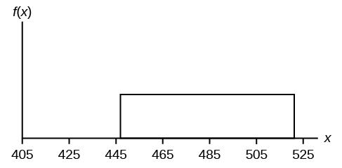
The total duration of baseball games in the major league in the 2011 season is uniformly distributed between 447 hours and 521 hours inclusive.

Find $a$ and $b$ and describe what they represent.
Write the distribution.
Find the mean and the standard deviation.
What is the probability that the duration of games for a team for the 2011 season is between 480 and 500 hours?
What is the 65 th percentile for the duration of games for a team for the 2011 season?
$a$ is $447$, and $b$ is $521$. a is the minimum duration of games for a team for the 2011 season, and $b$ is the maximum duration of games for a team for the 2011 season.
$X \sim U(447, 521)$.

Figure 5.3.1.

$P(480 < x < 500) = 0.2703$
65 th percentile is 495.1 hours.

Example 5.3.4

Suppose the time it takes a nine-year old to eat a donut is between 0.5 and 4 minutes, inclusive. Let $X =$ the time, in minutes, it takes a nine-year old child to eat a donut. Then $X \sim U(0.5, 4)$.

a. The probability that a randomly selected nine-year old child eats a donut in at least two minutes is _______.

Exercise 5.3.4.1

b. Find the probability that a different nine-year old child eats a donut in more than two minutes given that the child has already been eating the donut for more than 1.5 minutes.

The second question has a conditional probability. You are asked to find the probability that a nine-year old child eats a donut in more than two minutes given that the child has already been eating the donut for more than 1.5 minutes. Solve the problem two different ways (see Example ). You must reduce the sample space. First way : Since you know the child has already been eating the donut for more than 1.5 minutes, you are no longer starting at a = 0.5 minutes. Your starting point is 1.5 minutes.

Write a new $f(x)$:

$f(x) = \frac{1}{4-1.5} = \frac{2}{5}$ for $1.5 \leq x \leq 4$.

Find $P(x > 2|x > 1.5)$. Draw a graph.

$P(x > 2|x > 1.5) = (\text{base})(\text{new height}) = (4 − 2)(25)\left(\frac{2}{5}\right) =$ ?

b. $\frac{4}{5}$

The probability that a nine-year old child eats a donut in more than two minutes given that the child has already been eating the donut for more than 1.5 minutes is $\frac{4}{5}$.

Second way: Draw the original graph for $X \sim U(0.5, 4)$. Use the conditional formula

$P(x > 2 | x > 1.5) = \frac{P(x > 2 \text{AND} x > 1.5)}{P(x > 1.5)} = \frac{P(x>2)}{P(x>1.5)} = \frac{\frac{2}{3.5}}{\frac{2.5}{3.5}} = 0.8 = \frac{4}{5}$

Exercise 5.3.5

Suppose the time it takes a student to finish a quiz is uniformly distributed between six and 15 minutes, inclusive. Let $X =$ the time, in minutes, it takes a student to finish a quiz. Then $X \sim U(6, 15)$.

Find the probability that a randomly selected student needs at least eight minutes to complete the quiz. Then find the probability that a different student needs at least eight minutes to finish the quiz given that she has already taken more than seven minutes.

$P(x > 8) = 0.7778$

$P(x > 8 | x > 7) = 0.875$

Example 5.3.5

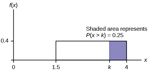
Ace Heating and Air Conditioning Service finds that the amount of time a repairman needs to fix a furnace is uniformly distributed between 1.5 and four hours. Let $x =$ the time needed to fix a furnace. Then $x \sim U(1.5, 4)$.

Find the probability that a randomly selected furnace repair requires more than two hours.
Find the probability that a randomly selected furnace repair requires less than three hours.
Find the 30 th percentile of furnace repair times.
The longest 25% of furnace repair times take at least how long? (In other words: find the minimum time for the longest 25% of repair times.) What percentile does this represent?
Find the mean and standard deviation

a. To find $f(x): f(x) = \frac{1}{4-1.5} = \frac{1}{2.5}$ so $f(x) = 0.4$

$P(x > 2) = (\text{base})(\text{height}) = (4 – 2)(0.4) = 0.8$

b. $P(x < 3) = (\text{base})(\text{height}) = (3 – 1.5)(0.4) = 0.6$

The graph of the rectangle showing the entire distribution would remain the same. However the graph should be shaded between $x = 1.5$ and $x = 3$. Note that the shaded area starts at $x = 1.5$ rather than at $x = 0$; since $X \sim U(1.5, 4)$, $x$ can not be less than 1.5.

$P(x < k) = 0.30$ $P(x < k) = (\text{base})(\text{height}) = (k – 1.5)(0.4)$ $0.3 = (k – 1.5) (0.4)$ ; Solve to find $k$: $0.75 = k – 1.5$, obtained by dividing both sides by 0.4 $k = 2.25$ , obtained by adding 1.5 to both sides

The 30 th percentile of repair times is 2.25 hours. 30% of repair times are 2.5 hours or less.

$P(x > k) = 0.25$ $P(x > k) = (\text{base})(\text{height}) = (4 – k)(0.4)$ $0.25 = (4 – k)(0.4)$ ; Solve for $k$: $0.625 = 4 − k$, obtained by dividing both sides by 0.4 $−3.375 = −k$, obtained by subtracting four from both sides: $k = 3.375$ The longest 25% of furnace repairs take at least 3.375 hours (3.375 hours or longer).

Note: Since 25% of repair times are 3.375 hours or longer, that means that 75% of repair times are 3.375 hours or less. 3.375 hours is the 75 th percentile of furnace repair times.

e. $\mu = \frac{a+b}{2}$ and $\sigma = \sqrt{\frac{(b-a)^{2}}{12}}$

$\mu = \frac{1.5+4}{2} = 2.75$ hours and $\sigma = \sqrt{\frac{(4-1.5)^{2}}{12}} = 0.7217$ hours

Exercise 5.3.6

The amount of time a service technician needs to change the oil in a car is uniformly distributed between 11 and 21 minutes. Let $X =$ the time needed to change the oil on a car.

Write the random variable $X$ in words. $X =$ __________________.
Graph the distribution.
Find $P(x > 19)$.
Find the 50 th percentile.
Let $X =$ the time needed to change the oil in a car.
$X \sim U(11, 21)$.

Figure 5.3.7.

$P(x > 19) = 0.2$
the 50 th percentile is 16 minutes.

Chapter Review

If $X$ has a uniform distribution where $a < x < b$ or $a \leq x \leq b$, then $X$ takes on values between $a$ and $b$ (may include $a$ and $b$). All values $x$ are equally likely. We write $X \sim U(a, b)$. The mean of $X$ is $\mu = \frac{a+b}{2}$. The standard deviation of $X$ is $\sigma = \sqrt{\frac{(b-a)^{2}}{12}}$. The probability density function of $X$ is $f(x) = \frac{1}{b-a}$ for $a \leq x \leq b$. The cumulative distribution function of $X$ is $P(X \leq x) = \frac{x-a}{b-a}$. $X$ is continuous.

The probability $P(c < X < d)$ may be found by computing the area under $f(x)$, between $c$ and $d$. Since the corresponding area is a rectangle, the area may be found simply by multiplying the width and the height.

Formula Review

$X =$ a real number between $a$ and $b$ (in some instances, $X$ can take on the values $a$ and $b$). $a =$ smallest $X$; $b =$ largest $X$

$X \sim U(a, b)$

The mean is $\mu = \frac{a+b}{2}$

The standard deviation is $\sigma = \sqrt{\frac{(b-a)^{2}}{12}}$

Probability density function: $f(x) = \frac{1}{b-a} \text{for} a \leq X \leq b$

Area to the Left of $x$: $P(X < x) = (x – a)\left(\frac{1}{b-a}\right)$

Area to the Right of $x$: P($X$ > $x$) = (b – x)$\left(\frac{1}{b-a}\right)$

Area Between $c$ and $d$: $P(c < x < d) = (\text{base})(\text{height}) = (d – c)\left(\frac{1}{b-a}\right)$

Uniform: $X \sim U(a, b)$ where $a < x < b$

pdf: $f(x) = \frac{1}{b-a}$ for $a \leq x \leq b$
cdf: $P(X \leq x) = \frac{x-a}{b-a}$
mean $\mu = \frac{a+b}{2}$
standard deviation $\sigma = \sqrt{\frac{(b-a)^{2}}{12}}$
$P(c < X < d) = (d – c)\left(\frac{1}{b-a}\right)$

McDougall, John A. The McDougall Program for Maximum Weight Loss. Plume, 1995.

Use the following information to answer the next ten questions. The data that follow are the square footage (in 1,000 feet squared) of 28 homes.

The sample mean = 2.50 and the sample standard deviation = 0.8302.

The distribution can be written as $X \sim U(1.5, 4.5)$.

Exercise 5.3.7

What type of distribution is this?

Exercise 5.3.8

In this distribution, outcomes are equally likely. What does this mean?

It means that the value of x is just as likely to be any number between 1.5 and 4.5.

Exercise 5.3.9

What is the height of $f(x)$ for the continuous probability distribution?

Exercise 5.3.10

What are the constraints for the values of $x$?

$1.5 \leq x \leq 4.5$

Exercise 5.3.11

Graph $P(2 < x < 3)$.

Exercise 5.3.12

What is $P(2 < x < 3)$?

Exercise 5.3.13

What is $P(x < 3.5 | x < 4)$?

Exercise 5.3.14

What is $P(x = 1.5)$?

Exercise 5.3.15

What is the 90 th percentile of square footage for homes?

Exercise 5.3.16

Find the probability that a randomly selected home has more than 3,000 square feet given that you already know the house has more than 2,000 square feet.

Exercise 5.3.17

What is $a$? What does it represent?

Exercise 5.3.18

What is $b$? What does it represent?

$b$ is $12$, and it represents the highest value of $x$.

Exercise 5.3.19

What is the probability density function?

Exercise 5.3.20

What is the theoretical mean?

Exercise 5.3.21

What is the theoretical standard deviation?

Exercise 5.3.22

Draw the graph of the distribution for $P(x > 9)$.

Exercise 5.3.23

Find $P(x > 9)$.

Exercise 5.3.24

Find the 40 th percentile.

Use the following information to answer the next eleven exercises. The age of cars in the staff parking lot of a suburban college is uniformly distributed from six months (0.5 years) to 9.5 years.

Exercise 5.3.25

What is being measured here?

Exercise 5.3.26

In words, define the random variable $X$.

$X$ = The age (in years) of cars in the staff parking lot

Exercise 5.3.27

Are the data discrete or continuous?

Exercise 5.3.28

The interval of values for $x$ is ______.

Exercise 5.3.29

The distribution for $X$ is ______.

Exercise 5.3.30

Write the probability density function.

$f(x) = \frac{1}{9}$ where $x$ is between 0.5 and 9.5, inclusive.

Exercise 5.3.31

Graph the probability distribution.

Figure 5.3.10.

Lowest value for $\bar{x}$: _______
Highest value for $\bar{x}$: _______
Height of the rectangle: _______
Label for x -axis (words): _______
Label for y -axis (words): _______

Exercise 5.3.32

Find the average age of the cars in the lot.

$\mu$ = 5

Exercise 5.3.33

Find the probability that a randomly chosen car in the lot was less than four years old.

Figure 5.3.11.

Find the probability. $P(x < 4) =$ _______

Exercise 5.3.34

Considering only the cars less than 7.5 years old, find the probability that a randomly chosen car in the lot was less than four years old.

Figure 5.3.12.

Find the probability. $P(x < 4 | x < 7.5) =$ _______
Check student’s solution.
$\frac{3.5}{7}$

Exercise 5.3.35

What has changed in the previous two problems that made the solutions different

Exercise 5.3.36

Find the third quartile of ages of cars in the lot. This means you will have to find the value such that $\frac{3}{4}$, or 75%, of the cars are at most (less than or equal to) that age.

Figure 5.3.13.

Find the value $k$ such that $P(x < k) = 0.75$.
The third quartile is _______
Check student's solution.
$k = 7.25$

Contributors

Barbara Illowsky and Susan Dean (De Anza College) with many other contributing authors. Content produced by OpenStax College is licensed under a Creative Commons Attribution License 4.0 license. Download for free at http://cnx.org/contents/[email protected] .

Want to create or adapt books like this? Learn more about how Pressbooks supports open publishing practices.

Continuous Random Variables

The Uniform Distribution

OpenStaxCollege

[latexpage]

The data in [link] are 55 smiling times, in seconds, of an eight-week-old baby.

The sample mean = 11.49 and the sample standard deviation = 6.23.

We will assume that the smiling times, in seconds, follow a uniform distribution between zero and 23 seconds, inclusive. This means that any smiling time from zero to and including 23 seconds is equally likely . The histogram that could be constructed from the sample is an empirical distribution that closely matches the theoretical uniform distribution.

Let X = length, in seconds, of an eight-week-old baby’s smile.

The notation for the uniform distribution is

X ~ U ( a , b ) where a = the lowest value of x and b = the highest value of x .

The probability density function is f ( x ) = $\frac{1}{b-a}$ for a ≤ x ≤ b .

For this example, X ~ U (0, 23) and f ( x ) = $\frac{1}{23-0}$ for 0 ≤ X ≤ 23.

Formulas for the theoretical mean and standard deviation are

$\mu =\frac{a+b}{2}$ and $\sigma =\sqrt{\frac{{\left(b-a\right)}^{2}}{12}}$

For this problem, the theoretical mean and standard deviation are

μ = $\frac{0\text{ }+\text{ }23}{2}$ = 11.50 seconds and σ = $\sqrt{\frac{{\left(23\text{ }-\text{ }0\right)}^{2}}{12}}$ = 6.64 seconds.

Notice that the theoretical mean and standard deviation are close to the sample mean and standard deviation in this example.

The data that follow are the number of passengers on 35 different charter fishing boats. The sample mean = 7.9 and the sample standard deviation = 4.33. The data follow a uniform distribution where all values between and including zero and 14 are equally likely. State the values of a and b . Write the distribution in proper notation, and calculate the theoretical mean and standard deviation.

a is zero; b is 14; X ~ U (0, 14); μ = 7 passengers; σ = 4.04 passengers

a. Refer to [link] . What is the probability that a randomly chosen eight-week-old baby smiles between two and 18 seconds?

a. Find P (2 < x < 18).

P (2 < x < 18) = (base)(height) = (18 – 2)$\left(\frac{1}{23}\right)$ = $\left(\frac{16}{23}\right)$.

This graph shows a uniform distribution. The horizontal axis ranges from 0 to 15. The distribution is modeled by a rectangle extending from x = 0 to x = 15. A region from x = 2 to x = 18 is shaded inside the rectangle.

b. Find the 90 th percentile for an eight-week-old baby’s smiling time.

b. Ninety percent of the smiling times fall below the 90 th percentile, k , so P ( x < k ) = 0.90

$P\left(x<k\right)=0.90$

$\left(\text{base}\right)\left(\text{height}\right)=0.90$

$\text{(}k-0\text{)}\left(\frac{1}{23}\right)=0.90$

$k=\left(23\right)\left(0.90\right)=20.7$

This shows the graph of the function f(x) = 1/15. A horiztonal line ranges from the point (0, 1/15) to the point (15, 1/15). A vertical line extends from the x-axis to the end of the line at point (15, 1/15) creating a rectangle. A region is shaded inside the rectangle from x = 0 to x = k. The shaded area represents P(x < k) = 0.90.

c. Find the probability that a random eight-week-old baby smiles more than 12 seconds KNOWING that the baby smiles MORE THAN EIGHT SECONDS .

Find P ( x > 12| x > 8) There are two ways to do the problem. For the first way , use the fact that this is a conditional and changes the sample space. The graph illustrates the new sample space. You already know the baby smiled more than eight seconds.

Write a new f ( x ): f ( x ) = $\frac{1}{23\text{ }-\text{ 8}}$ = $\frac{1}{15}$

for 8 < x < 23

P ( x > 12| x > 8) = (23 − 12)$\left(\frac{1}{15}\right)$ = $\left(\frac{11}{15}\right)$

f(X)=1/15 graph displaying a boxed region consisting of a horizontal line extending to the right from point 1/15 on the y-axis, a vertical upward line from points 8 and 23 on the x-axis, and the x-axis. A shaded region from points 12-23 occurs within this area.

For the second way , use the conditional formula from Probability Topics with the original distribution X ~ U (0, 23):

P ( A | B ) = $\frac{P\left(A\text{ AND }B\right)}{P\left(B\right)}$

For this problem, A is ( x > 12) and B is ( x > 8).

So, P ( x > 12 | x > 8) = $\frac{\left(x>12\text{ AND }x>8\right)}{P\left(x>8\right)}=\frac{P\left(x>12\right)}{P\left(x>8\right)}=\frac{\frac{11}{23}}{\frac{15}{23}}=\frac{11}{15}$

This shows the graph of the function f(x) = 1/23. A horiztonal line ranges from the point (0, 1/23) to the point (23, 1/23). A vertical line extends from the x-axis to the end of the line at point (23, 1/23) creating a rectangle. Vertical lines extend from the horizontal axis to the graph at x = 8 and x = 12.

A distribution is given as X ~ U (0, 20). What is P (2 < x < 18)? Find the 90 th percentile.

P (2 < x < 18) = 0.8; 90 th percentile = 18

The amount of time, in minutes, that a person must wait for a bus is uniformly distributed between zero and 15 minutes, inclusive.

a. What is the probability that a person waits fewer than 12.5 minutes?

a. Let X = the number of minutes a person must wait for a bus. a = 0 and b = 15. X ~ U (0, 15). Write the probability density function. f ( x ) = $\frac{1}{15\text{ }-\text{ }0}$ = $\frac{1}{15}$ for 0 ≤ x ≤ 15.

Find P ( x < 12.5). Draw a graph.

$P\left(x<k\right)=\left(\text{base}\right)\left(\text{height}\right)=\left(12.5-0\right)\left(\frac{1}{15}\right)=0.8333$

The probability a person waits less than 12.5 minutes is 0.8333.

b. On the average, how long must a person wait? Find the mean, μ , and the standard deviation, σ .

b. μ = $\frac{a\text{ }+\text{ }b}{2}$ = $\frac{15\text{ }+\text{ }0}{2}$ = 7.5. On the average, a person must wait 7.5 minutes.

σ = $\sqrt{\frac{\left(b-a{\right)}^{2}}{12}}=\sqrt{\frac{\left(\mathrm{15}-0{\right)}^{2}}{12}}$ = 4.3. The Standard deviation is 4.3 minutes.

c. Ninety percent of the time, the time a person must wait falls below what value?

c. Find the 90 th percentile. Draw a graph. Let k = the 90 th percentile.

$P\left(x<k\right)=\left(\text{base}\right)\left(\text{height}\right)=\left(k-0\right)\left(\frac{1}{15}\right)$

$0.90=\left(k\right)\left(\frac{1}{15}\right)$

$k=\left(0.90\right)\left(15\right)=13.5$

k is sometimes called a critical value.

The 90 th percentile is 13.5 minutes. Ninety percent of the time, a person must wait at most 13.5 minutes.

The total duration of baseball games in the major league in the 2011 season is uniformly distributed between 447 hours and 521 hours inclusive.

Find a and b and describe what they represent.
Write the distribution.
Find the mean and the standard deviation.
What is the probability that the duration of games for a team for the 2011 season is between 480 and 500 hours?
What is the 65 th percentile for the duration of games for a team for the 2011 season?
a is 447, and b is 521. a is the minimum duration of games for a team for the 2011 season, and b is the maximum duration of games for a team for the 2011 season.
X ~ U (447, 521).

graphical representation uniformly distributed

P (480 < x < 500) = 0.2703
65 th percentile is 495.1 hours.

Suppose the time it takes a nine-year old to eat a donut is between 0.5 and 4 minutes, inclusive. Let X = the time, in minutes, it takes a nine-year old child to eat a donut. Then X ~ U (0.5, 4).

a. The probability that a randomly selected nine-year old child eats a donut in at least two minutes is _______.

b. Find the probability that a different nine-year old child eats a donut in more than two minutes given that the child has already been eating the donut for more than 1.5 minutes.

The second question has a conditional probability . You are asked to find the probability that a nine-year old child eats a donut in more than two minutes given that the child has already been eating the donut for more than 1.5 minutes. Solve the problem two different ways (see [link] ). You must reduce the sample space. First way : Since you know the child has already been eating the donut for more than 1.5 minutes, you are no longer starting at a = 0.5 minutes. Your starting point is 1.5 minutes.

Write a new f ( x ):

f ( x ) = $\frac{1}{4-1.5}$ = $\frac{2}{5}$ for 1.5 ≤ x ≤ 4.

Find P ( x > 2| x > 1.5). Draw a graph.

f(X)=2/5 graph displaying a boxed region consisting of a horizontal line extending to the right from point 2/5 on the y-axis, a vertical upward line from points 1.5 and 4 on the x-axis, and the x-axis. A shaded region from points 2-4 occurs within this area.

P ( x > 2 | x > 1.5) = (base)(new height) = (4 − 2)$\left(\frac{2}{5}\right)$= ?

b. $\frac{4}{5}$

The probability that a nine-year old child eats a donut in more than two minutes given that the child has already been eating the donut for more than 1.5 minutes is $\frac{4}{5}$.

Second way: Draw the original graph for X ~ U (0.5, 4). Use the conditional formula

P ( x > 2| x > 1.5) = $ \frac{P\left(x>2\text{ AND }x>1.5\right)}{P\left(x>\text{1}\text{.5}\right)}=\frac{P\left(x>2\right)}{P\left(x>1.5\right)}=\frac{\frac{2}{3.5}}{\frac{2.5}{3.5}}=\text{0}\text{.8}=\frac{4}{5}$

Suppose the time it takes a student to finish a quiz is uniformly distributed between six and 15 minutes, inclusive. Let X = the time, in minutes, it takes a student to finish a quiz. Then X ~ U (6, 15).

P ( x > 8) = 0.7778

P ( x > 8 | x > 7) = 0.875

Ace Heating and Air Conditioning Service finds that the amount of time a repairman needs to fix a furnace is uniformly distributed between 1.5 and four hours. Let x = the time needed to fix a furnace. Then x ~ U (1.5, 4).

Find the probability that a randomly selected furnace repair requires more than two hours.
Find the probability that a randomly selected furnace repair requires less than three hours.
Find the 30 th percentile of furnace repair times.
The longest 25% of furnace repair times take at least how long? (In other words: find the minimum time for the longest 25% of repair times.) What percentile does this represent?
Find the mean and standard deviation

a. To find f ( x ): f ( x ) = $\frac{1}{4\text{ }-\text{ }1.5}$ = $\frac{1}{2.5}$ so f ( x ) = 0.4

P ( x > 2) = (base)(height) = (4 – 2)(0.4) = 0.8

This shows the graph of the function f(x) = 0.4. A horiztonal line ranges from the point (1.5, 0.4) to the point (4, 0.4). Vertical lines extend from the x-axis to the graph at x = 1.5 and x = 4 creating a rectangle. A region is shaded inside the rectangle from x = 2 to x = 4.

b. P ( x < 3) = (base)(height) = (3 – 1.5)(0.4) = 0.6

The graph of the rectangle showing the entire distribution would remain the same. However the graph should be shaded between x = 1.5 and x = 3. Note that the shaded area starts at x = 1.5 rather than at x = 0; since X ~ U (1.5, 4), x can not be less than 1.5.

P ( x < k ) = 0.30

P ( x < k ) = (base)(height) = ( k – 1.5)(0.4)

0.3 = ( k – 1.5) (0.4) ; Solve to find k :

0.75 = k – 1.5, obtained by dividing both sides by 0.4

k = 2.25 , obtained by adding 1.5 to both sides

P ( x > k ) = 0.25

P ( x > k ) = (base)(height) = (4 – k )(0.4)

0.25 = (4 – k )(0.4) ; Solve for k :

0.625 = 4 − k ,

obtained by dividing both sides by 0.4

−3.375 = − k ,

obtained by subtracting four from both sides: k = 3.375

The longest 25% of furnace repairs take at least 3.375 hours (3.375 hours or longer).

e. $\mu =\frac{a+b}{2}$ and $\sigma =\sqrt{\frac{{\left(b-a\right)}^{2}}{12}}$

$\mu =\frac{1.5+4}{2}=2.75$ hours and $\sigma =\sqrt{\frac{{\left(4–1.5\right)}^{2}}{12}}=0.7217$ hours

The amount of time a service technician needs to change the oil in a car is uniformly distributed between 11 and 21 minutes. Let X = the time needed to change the oil on a car.

Write the random variable X in words. X = __________________.
Graph the distribution.
Find P ( x > 19).
Find the 50 th percentile.
Let X = the time needed to change the oil in a car.
X ~ U (11, 21).

This graph shows a uniform distribution. The horizontal axis ranges from 405 to 525. The distribution is modeled by a rectangle extending from x = 447 to x = 521.

P ( x > 19) = 0.2
the 50 th percentile is 16 minutes.

Chapter Review

If X has a uniform distribution where a < x < b or a ≤ x ≤ b , then X takes on values between a and b (may include a and b ). All values x are equally likely. We write X ∼ U ( a , b ). The mean of X is $\mu =\frac{a+b}{2}$. The standard deviation of X is $\sigma =\sqrt{\frac{{\left(b-a\right)}^{2}}{12}}$. The probability density function of X is $f\left(x\right)=\frac{1}{b-a}$ for a ≤ x ≤ b . The cumulative distribution function of X is P ( X ≤ x ) = $\frac{x-a}{b-a}$. X is continuous.

The graph shows a rectangle with total area equal to 1. The rectangle extends from x = a to x = b on the x-axis and has a height of 1/(b-a).

The probability P ( c < X < d ) may be found by computing the area under f ( x ), between c and d . Since the corresponding area is a rectangle, the area may be found simply by multiplying the width and the height.

Formula Review

X = a real number between a and b (in some instances, X can take on the values a and b ). a = smallest X ; b = largest X

X ~ U (a, b)

The mean is $\mu =\frac{a+b}{2}$

The standard deviation is $\sigma =\sqrt{\frac{{\left(b\text{ – }a\right)}^{2}}{12}}$

Probability density function: $f\left(x\right)=\frac{1}{b-a}$ for $a\le X\le b$

Area to the Left of x : P ( X < x ) = ( x – a )$\left(\frac{1}{b-a}\right)$

Area to the Right of x : P ( X > x ) = ( b – x )$\left(\frac{1}{b-a}\right)$

Area Between c and d : P ( c < x < d ) = (base)(height) = ( d – c )$\left(\frac{1}{b-a}\right)$

Uniform: X ~ U ( a , b ) where a < x < b

pdf: $f\left(x\right)=\frac{1}{b-a}$ for a ≤ x ≤ b
cdf: P ( X ≤ x ) = $\frac{x-a}{b-a}$
mean µ = $\frac{a+b}{2}$
standard deviation σ $=\sqrt{\frac{{\left(b-a\right)}^{2}}{12}}$
P ( c < X < d ) = ( d – c )$\left(\frac{1}{b–a}\right)$

McDougall, John A. The McDougall Program for Maximum Weight Loss. Plume, 1995.

Use the following information to answer the next ten questions. The data that follow are the square footage (in 1,000 feet squared) of 28 homes.

The sample mean = 2.50 and the sample standard deviation = 0.8302.

The distribution can be written as X ~ U (1.5, 4.5).

What type of distribution is this?

In this distribution, outcomes are equally likely. What does this mean?

It means that the value of x is just as likely to be any number between 1.5 and 4.5.

What is the height of f ( x ) for the continuous probability distribution?

What are the constraints for the values of x ?

1.5 ≤ x ≤ 4.5

Graph P (2 < x < 3).

What is P (2 < x < 3)?

What is P (x < 3.5| x < 4)?

What is P ( x = 1.5)?

What is the 90 th percentile of square footage for homes?

Find the probability that a randomly selected home has more than 3,000 square feet given that you already know the house has more than 2,000 square feet.

Use the following information to answer the next eight exercises. A distribution is given as X ~ U (0, 12).

What is a ? What does it represent?

What is b ? What does it represent?

b is 12, and it represents the highest value of x .

What is the probability density function?

What is the theoretical mean?

What is the theoretical standard deviation?

Draw the graph of the distribution for P ( x > 9).

This graph shows a uniform distribution. The horizontal axis ranges from 0 to 12. The distribution is modeled by a rectangle extending from x = 0 to x = 12. A region from x = 9 to x = 12 is shaded inside the rectangle.

Find P ( x > 9).

Find the 40 th percentile.

Use the following information to answer the next eleven exercises. The age of cars in the staff parking lot of a suburban college is uniformly distributed from six months (0.5 years) to 9.5 years.

What is being measured here?

In words, define the random variable X .

X = The age (in years) of cars in the staff parking lot

Are the data discrete or continuous?

The interval of values for x is ______.

The distribution for X is ______.

Write the probability density function.

f ( x ) = $\frac{1}{9}$ where x is between 0.5 and 9.5, inclusive.

Graph the probability distribution.

This is a blank graph template. The vertical and horizontal axes are unlabeled.

Lowest value for $\overline{x}$: _______
Highest value for $\overline{x}$: _______
Height of the rectangle: _______
Label for x -axis (words): _______
Label for y -axis (words): _______

Find the average age of the cars in the lot.

Find the probability that a randomly chosen car in the lot was less than four years old.

Blank graph with vertical and horizontal axes.

Find the probability. P ( x < 4) = _______

Considering only the cars less than 7.5 years old, find the probability that a randomly chosen car in the lot was less than four years old.

Find the probability. P ( x < 4| x < 7.5) = _______
Check student’s solution.
$\frac{3.5}{7}$

What has changed in the previous two problems that made the solutions different?

Find the third quartile of ages of cars in the lot. This means you will have to find the value such that $\frac{3}{4}$, or 75%, of the cars are at most (less than or equal to) that age.

Find the value k such that P ( x < k ) = 0.75.
The third quartile is _______
Check student’s solution.

For each probability and percentile problem, draw the picture.

Births are approximately uniformly distributed between the 52 weeks of the year. They can be said to follow a uniform distribution from one to 53 (spread of 52 weeks).

X ~ _________
f ( x ) = _________
μ = _________
σ = _________
Find the probability that a person is born at the exact moment week 19 starts. That is, find P ( x = 19) = _________
P (2 < x < 31) = _________
Find the probability that a person is born after week 40.
P (12 < x | x < 28) = _________
Find the 70 th percentile.
Find the minimum for the upper quarter.

A random number generator picks a number from one to nine in a uniform manner.

P (3.5 < x < 7.25) = _________
P ( x > 5.67)
P ( x > 5| x > 3) = _________
Find the 90 th percentile.
X ~ U (1, 9)
$f\left(x\right)=\frac{1}{8}$ where $1\le x\le 9$
$\frac{15}{32}$
$\frac{333}{800}$
$\frac{2}{3}$

According to a study by Dr. John McDougall of his live-in weight loss program at St. Helena Hospital, the people who follow his program lose between six and 15 pounds a month until they approach trim body weight. Let’s suppose that the weight loss is uniformly distributed. We are interested in the weight loss of a randomly selected individual following the program for one month.

Define the random variable. X = _________
Find the probability that the individual lost more than ten pounds in a month.
Suppose it is known that the individual lost more than ten pounds in a month. Find the probability that he lost less than 12 pounds in the month.
P (7 < x < 13| x > 9) = __________. State this in a probability question, similarly to parts g and h, draw the picture, and find the probability.

A subway train on the Red Line arrives every eight minutes during rush hour. We are interested in the length of time a commuter must wait for a train to arrive. The time follows a uniform distribution.

Define the random variable. X = _______
X ~ _______
f ( x ) = _______
μ = _______
σ = _______
Find the probability that the commuter waits less than one minute.
Find the probability that the commuter waits between three and four minutes.
Sixty percent of commuters wait more than how long for the train? State this in a probability question, similarly to parts g and h, draw the picture, and find the probability.
X represents the length of time a commuter must wait for a train to arrive on the Red Line.
X ~ U (0, 8)
$f\left(x\right)=\frac{1}{8}$ where ≤ x ≤ 8
$\frac{1}{8}$

The age of a first grader on September 1 at Garden Elementary School is uniformly distributed from 5.8 to 6.8 years. We randomly select one first grader from the class.

Find the probability that she is over 6.5 years old.
Find the probability that she is between four and six years old.
Find the 70 th percentile for the age of first graders on September 1 at Garden Elementary School.

Use the following information to answer the next three exercises. The Sky Train from the terminal to the rental–car and long–term parking center is supposed to arrive every eight minutes. The waiting times for the train are known to follow a uniform distribution.

What is the average waiting time (in minutes)?

Find the 30 th percentile for the waiting times (in minutes).

The probability of waiting more than seven minutes given a person has waited more than four minutes is?

The time (in minutes) until the next bus departs a major bus depot follows a distribution with f ( x ) = $\frac{1}{20}$ where x goes from 25 to 45 minutes.

Define the random variable. X = ________
X ~ ________
The distribution is ______________ (name of distribution). It is _____________ (discrete or continuous).
μ = ________
σ = ________
Find the probability that the time is at most 30 minutes. Sketch and label a graph of the distribution. Shade the area of interest. Write the answer in a probability statement.
Find the probability that the time is between 30 and 40 minutes. Sketch and label a graph of the distribution. Shade the area of interest. Write the answer in a probability statement.
P (25 < x < 55) = _________. State this in a probability statement, similarly to parts g and h, draw the picture, and find the probability.
Find the 90 th percentile. This means that 90% of the time, the time is less than _____ minutes.
Find the 75 th percentile. In a complete sentence, state what this means. (See part j.)
Find the probability that the time is more than 40 minutes given (or knowing that) it is at least 30 minutes.

Suppose that the value of a stock varies each day from 💲16 to 💲25 with a uniform distribution.

Find the probability that the value of the stock is more than 💲19.
Find the probability that the value of the stock is between 💲19 and 💲22.
Find the upper quartile – 25% of all days the stock is above what value? Draw the graph.
Given that the stock is greater than 💲18, find the probability that the stock is more than 💲21.

P ( X > 19) = (25 – 19) $\left(\frac{1}{9}\right)$ = $\frac{6}{9}$ = $\frac{2}{3}$.

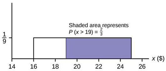
The area must be 0.25, and 0.25 = (width)$\left(\frac{1}{9}\right)$, so width = (0.25)(9) = 2.25. Thus, the value is 25 – 2.25 = 22.75.

A fireworks show is designed so that the time between fireworks is between one and five seconds, and follows a uniform distribution.

Find the average time between fireworks.
Find probability that the time between fireworks is greater than four seconds.

The number of miles driven by a truck driver falls between 300 and 700, and follows a uniform distribution.

Find the probability that the truck driver goes more than 650 miles in a day.
Find the probability that the truck drivers goes between 400 and 650 miles in a day.
At least how many miles does the truck driver travel on the furthest 10% of days?
P ( X > 650) = $\frac{700-650}{700-300}=\frac{500}{400}=\frac{1}{8}$ = 0.125.
P (400 < X < 650) = $\frac{700-650}{700-300}=\frac{250}{400}$ = 0.625
0.10 = $\frac{\text{width}}{\text{700}-\text{300}}$, so width = 400(0.10) = 40. Since 700 – 40 = 660, the drivers travel at least 660 miles on the furthest 10% of days.

Module 5: Continuous Random Variables

The uniform distribution, learning outcomes.

Recognize the uniform probability distribution and apply it appropriately

The data in the table below are 55 smiling times, in seconds, of an eight-week-old baby.

The sample mean[latex]=11.49[/latex] and the sample standard deviation[latex]=6.23[/latex].

Let [latex]X=[/latex] length, in seconds, of an eight-week-old baby’s smile.

The notation for the uniform distribution is [latex]X{\sim}U(a,b)[/latex] where [latex]a=[/latex] the lowest value of x and [latex]b=[/latex] the highest value of x .

The probability density function is [latex]{f{{({x})}}}=\frac{{1}}{{{b}-{a}}}[/latex] for [latex]a{\leq}x{\leq}b[/latex].

For this example, [latex]X{\sim}U(0,23)[/latex] and [latex]{f{{({x})}}}=\frac{{1}}{{{23}-{0}}}[/latex] for [latex]0{\leq}X{\leq}23[/latex].

Formulas for the theoretical mean and standard deviation are [latex]{\mu}=\frac{{{a}+{b}}}{{2}}{\quad\text{and}\quad}{\sigma}=\sqrt{{\frac{{{({b}-{a})}^{{2}}}}{{12}}}}[/latex]

For this problem, the theoretical mean and standard deviation are [latex]{\mu}=\frac{{{0}+{23}}}{{2}}={11.50} \text{ seconds}{\quad\text{and}\quad}{\sigma}=\sqrt{{\frac{{{({23}-{0})}^{{2}}}}{{12}}}}={6.64} \text{ seconds}[/latex]

Notice that the theoretical mean and standard deviation are close to the sample mean and standard deviation in this example.

The data that follow are the number of passengers on 35 different charter fishing boats. The sample mean [latex]=7.9[/latex] and the sample standard deviation [latex]=4.33[/latex]. The data follow a uniform distribution where all values between and including zero and 14 are equally likely. State the values of a and b . Write the distribution in proper notation, and calculate the theoretical mean and standard deviation.

a is zero; b is 14; [latex]X{\sim}U(0,14)[/latex]; [latex]\mu=7[/latex] passengers; [latex]\sigma=4.04[/latex] passengers

Refer to the previous example. What is the probability that a randomly chosen eight-week-old baby smiles between two and 18 seconds?
Find the 90th percentile for an eight-week-old baby’s smiling time.
Find the probability that a random eight-week-old baby smiles more than 12 seconds knowing that the baby smiles more than eight seconds .

A distribution is given as [latex]X{\sim}U(0,20)[/latex]. What is [latex]P(2<x<18)[/latex]? Find the 90th percentile.

[latex]P(2<x<18)=0.8[/latex]; 90th percentile[latex]=18[/latex]

The amount of time, in minutes, that a person must wait for a bus is uniformly distributed between zero and 15 minutes, inclusive.

What is the probability that a person waits fewer than 12.5 minutes?
On the average, how long must a person wait? Find the mean, μ , and the standard deviation, σ .
Ninety percent of the time, the time a person must wait falls below what value? This asks for the 90th percentile .

[latex]{\mu}=\frac{{{a}+{b}}}{{2}}=\frac{{{15}+{0}}}{{2}}={7.5}[/latex]. On the average, a person must wait 7.5 minutes.[latex]{\sigma}=\sqrt{{\frac{{{({b}-{a})}^{{2}}}}{{12}}}}=\sqrt{{\frac{{{({15}-{0})}^{{2}}}}{{12}}}}={4.3}[/latex]The standard deviation is 4.3 minutes.

The total duration of baseball games in the major league in the 2011 season is uniformly distributed between 447 hours and 521 hours inclusive.

Find a and b and describe what they represent.
Write the distribution.
Find the mean and the standard deviation.
What is the probability that the duration of games for a team for the 2011 season is between 480 and 500 hours?
What is the 65th percentile for the duration of games for a team for the 2011 season?
a is 447, and b is 521. a is the minimum duration of games for a team for the 2011 season, and b is the maximum duration of games for a team for the 2011 season.
X ~ U (447, 521).

P (480 < x < 500) = 0.2703
65th percentile is 495.1 hours.

Suppose the time it takes a nine-year old to eat a donut is between 0.5 and 4 minutes, inclusive. Let X = the time, in minutes, it takes a nine-year old child to eat a donut. Then X ~ U (0.5, 4).

The probability that a randomly selected nine-year old child eats a donut in at least two minutes is _______.
Find the probability that a different nine-year old child eats a donut in more than two minutes given that the child has already been eating the donut for more than 1.5 minutes.

Second way: Draw the original graph for X ~ U (0.5, 4). Use the conditional formula[latex]{P}{({x}{>}{2}{mid}{x}{>}{1.5})}=\frac{{{P}{({x}{>}{2} \text{ AND } {x}{>}{1.5})}}}{{{P}{({x}{>}{1.5})}}}=\frac{{{P}{({x}{>}{2})}}}{{{P}{({x}{>}{1.5})}}}=\frac{{\frac{{2}}{{3.5}}}}{{\frac{{2.5}}{{3.5}}}}={0.8}=\frac{{4}}{{5}}[/latex]

P ( x > 8) = 0.7778

P ( x > 8 | x > 7) = 0.875

Find the probability that a randomly selected furnace repair requires more than two hours.
Find the probability that a randomly selected furnace repair requires less than three hours.
Find the 30th percentile of furnace repair times.
The longest 25% of furnace repair times take at least how long? (In other words: find the minimum time for the longest 25% of repair times.) What percentile does this represent?
Find the mean and standard deviation

−3.375 = − k , obtained by subtracting four from both sides: k = 3.375

The longest 25% of furnace repairs take at least 3.375 hours (3.375 hours or longer).

Note: Since 25% of repair times are 3.375 hours or longer, that means that 75% of repair times are 3.375 hours or less. 3.375 hours is the 75th percentile of furnace repair times.

[latex]{\mu}={\frac{a+b}{2}}\text{ and }{\sigma}=\sqrt{\frac{(b-a)^2}{12}}[/latex] [latex]{\mu}=\frac{1.5+4}{2}=2.75\text{ hours and }{\sigma}=\sqrt{\frac{(4-1.5)^2}{12}}= 0.7217 \text{ hours}[/latex]

The amount of time a service technician needs to change the oil in a car is uniformly distributed between 11 and 21 minutes. Let X = the time needed to change the oil on a car.

Write the random variable X in words. X = __________________.
Graph the distribution.
Find P ( x > 19).
Find the 50th percentile.
Let X = the time needed to change the oil in a car.
X ~ U (11, 21).

P ( x > 19) = 0.2
the 50th percentile is 16 minutes.

McDougall, John A. The McDougall Program for Maximum Weight Loss. Plume, 1995.

Concept Review

If X has a uniform distribution where a < x < b or a ≤ x ≤ b , then X takes on values between a and b (may include a and b ). All values x are equally likely. We write X ∼ U ( a , b ). The mean of X is [latex]{\mu}=\frac{{{a}+{b}}}{{2}}[/latex]. X is continuous.

Formula Review

X = a real number between a and b (in some instances, X can take on the values a and b ). a = smallest X ; b = largest X

X ~ U (a, b)

The mean is [latex]\mu=\frac{{{a}+{b}}}{{2}}[/latex]

The standard deviation is [latex]\sigma=\sqrt{{\frac{{({b}-{a})}^{{2}}}{{12}}}}[/latex]

Probability density function: [latex]{f{{({x})}}}=\frac{{1}}{{{b}-{a}}} \text{ for } {a}\leq{X}\leq{b}[/latex]

Area to the Left of x : [latex]{P}{({X}{<}{x})}={({x}-{a})}{(\frac{{1}}{{{b}-{a}}})}[/latex]

Area to the Right of x : [latex]{P}{({X}{>}{x})}={({b}-{x})}{(\frac{{1}}{{{b}-{a}}})}[/latex]

Area Between c and d : [latex]{P}{({c}{<}{x}{<}{d})}={(\text{base})}{(\text{height})}={({d}-{c})}{(\frac{{1}}{{{b}-{a}}})}[/latex]

Uniform: X ~ U ( a , b ) where a < x < b

pdf: [latex]{f{{({x})}}}=\frac{{1}}{{{b}-{a}}}[/latex] for a ≤ x ≤ b
cdf: P ( X ≤ x ) = [latex]\frac{{{x}-{a}}}{{{b}-{a}}}[/latex]
mean: [latex]\mu=\frac{{{a}+{b}}}{{2}}[/latex]
standard deviation: [latex]\sigma=\sqrt{{\frac{{({b}-{a})}^{{2}}}{{12}}}}[/latex]
P ( c < X < d ) = ( d – c )
OpenStax, Statistics, The Uniform Distribution. Provided by : OpenStax. Located at : http://cnx.org/contents/[email protected]:36/Introductory_Statistics . License : CC BY: Attribution
Introductory Statistics . Authored by : Barbara Illowski, Susan Dean. Provided by : Open Stax. Located at : http://cnx.org/contents/[email protected] . License : CC BY: Attribution . License Terms : Download for free at http://cnx.org/contents/[email protected]

Uniform distribution

by Marco Taboga , PhD

A continuous random variable has a uniform distribution if all the values belonging to its support have the same probability density.

Table of contents

Expected value

Moment generating function, characteristic function, distribution function, density plots, plot 1 - different supports but same length, plot 2 - different supports and different lengths, solved exercises.

The uniform distribution is characterized as follows.

A random variable having a uniform distribution is also called a uniform random variable. Sometimes, we also say that it has a rectangular distribution or that it is a rectangular random variable .

To better understand the uniform distribution, you can have a look at its density plots .

This section shows the plots of the densities of some uniform random variables, in order to demonstrate how the uniform density changes by changing its parameters.

The following plot contains the graphs of two uniform probability density functions:

The two random variables have different supports, but their two supports have the same length. Therefore, since the uniform density is constant and inversely proportional to the length of the support, the two random variables have the same constant density over their respective supports.

Below you can find some exercises with explained solutions.

How to cite

Please cite as:

Taboga, Marco (2021). "Uniform distribution", Lectures on probability theory and mathematical statistics. Kindle Direct Publishing. Online appendix. https://www.statlect.com/probability-distributions/uniform-distribution.

Most of the learning materials found on this website are now available in a traditional textbook format.

Normal distribution
Permutations
Mean square convergence
Independent events
Multivariate normal distribution
Binomial distribution
Central Limit Theorem
Multinomial distribution
Mathematical tools
Fundamentals of probability
Probability distributions
Asymptotic theory
Fundamentals of statistics
About Statlect
Cookies, privacy and terms of use
Precision matrix
Discrete random variable
Posterior probability
Binomial coefficient
Probability space
Power function
To enhance your privacy,
we removed the social buttons,
but don't forget to share .

5.2 The Uniform Distribution

Example 5.2

The data in Table 5.1 are 55 smiling times, in seconds, of an eight-week-old baby.

The sample mean = 11.65 and the sample standard deviation = 6.08.

We will assume that the smiling times, in seconds, follow a uniform distribution between zero and 23 seconds, inclusive. This means that any smiling time from zero to and including 23 seconds is equally likely . The histogram that could be constructed from the sample is an empirical distribution that closely matches the theoretical uniform distribution.

Let X = length, in seconds, of an eight-week-old baby's smile.

The notation for the uniform distribution is

X ~ U ( a , b ) where a = the lowest value of x and b = the highest value of x .

The probability density function is f ( x ) = 1 b − a 1 b − a for a ≤ x ≤ b .

For this example, x ~ U (0, 23) and f ( x ) = 1 23 − 0 1 23 − 0 for 0 ≤ X ≤ 23.

Formulas for the theoretical mean and standard deviation are

μ = a + b 2 μ = a + b 2 and σ = ( b − a ) 2 12 σ = ( b − a ) 2 12

For this problem, the theoretical mean and standard deviation are

μ = 0 + 23 2 0 + 23 2 = 11.50 seconds and σ = ( 23 − 0 ) 2 12 ( 23 − 0 ) 2 12 = 6.64 seconds.

Notice that the theoretical mean and standard deviation are close to the sample mean and standard deviation in this example.

The data that follow record the total weight, to the nearest pound, of fish caught by passengers on 35 different charter fishing boats on one summer day. The sample mean = 7.9 and the sample standard deviation = 4.33. The data follow a uniform distribution where all values between and including zero and 14 are equally likely. State the values of a and b . Write the distribution in proper notation, and calculate the theoretical mean and standard deviation.

Example 5.3

a. Refer to Example 5.2 . What is the probability that a randomly chosen eight-week-old baby smiles between two and 18 seconds?

P (2 < x < 18) = (base)(height) = (18 – 2) ( 1 23 ) ( 1 23 ) = 16 23 16 23 .

b. Find the 90 th percentile for an eight-week-old baby's smiling time.

b. Ninety percent of the smiling times fall below the 90 th percentile, k , so P ( x < k ) = 0.90.

P ( x < k ) = 0.90 P ( x < k ) = 0.90

( base ) ( height ) = 0.90 ( base ) ( height ) = 0.90

( k − 0 ) ( 1 23 ) = 0.90 ( k − 0 ) ( 1 23 ) = 0.90

k = ( 23 ) ( 0.90 ) = 20.7 k = ( 23 ) ( 0.90 ) = 20.7

c. Find the probability that a random eight-week-old baby smiles more than 12 seconds KNOWING that the baby smiles MORE THAN EIGHT SECONDS .

Write a new f ( x ): f ( x ) = 1 23 − 8 1 23 − 8 = 1 15 1 15 for 8 < x < 23

P ( x > 12| x > 8) = (23 − 12) ( 1 15 ) ( 1 15 ) = 11 15 11 15

For the second way , use the conditional formula from Probability Topics with the original distribution X ~ U (0, 23):

P ( A | B ) = P ( A AND B ) P ( B ) P ( A AND B ) P ( B )

For this problem, A is ( x > 12) and B is ( x > 8).

So, P ( x > 12 | x > 8) = P ( x > 12 AND x > 8 ) P ( x > 8 ) = P ( x > 12 ) P ( x > 8 ) = 11 23 15 23 = 11 15 P ( x > 12 AND x > 8 ) P ( x > 8 ) = P ( x > 12 ) P ( x > 8 ) = 11 23 15 23 = 11 15

A distribution is given as X ~ U (0, 20). What is P (2 < x < 18)? Find the 90 th percentile.

Example 5.4

The amount of time, in minutes, that a person must wait for a bus is uniformly distributed between zero and 15 minutes, inclusive.

a. What is the probability that a person waits fewer than 12.5 minutes?

b. On the average, how long must a person wait? Find the mean, μ , and the standard deviation, σ .

c. Ninety percent of the time, the time a person must wait falls below what value?

a. Let X = the number of minutes a person must wait for a bus. a = 0 and b = 15. X ~ U (0, 15). Write the probability density function. f ( x ) = 1 15 − 0 1 15 − 0 = 1 15 1 15 for 0 ≤ x ≤ 15.

Find P ( x < 12.5). Draw a graph.

P ( x < k ) = ( base ) ( height ) = ( 12.5 - 0 ) ( 1 15 ) = 0.8333 P ( x < k ) = ( base ) ( height ) = ( 12.5 - 0 ) ( 1 15 ) = 0.8333

The probability a person waits less than 12.5 minutes is 0.8333.

b. μ = a + b 2 a + b 2 = 15 + 0 2 15 + 0 2 = 7.5. On the average, a person must wait 7.5 minutes. σ = ( b - a ) 2 12 = ( 15 - 0 ) 2 12 ( b - a ) 2 12 = ( 15 - 0 ) 2 12 = 4.3. The Standard deviation is 4.3 minutes.

c. Find the 90 th percentile. Draw a graph. Let k = the 90 th percentile. P ( x < k ) = ( base ) ( height ) = ( k − 0 ) ( 1 15 ) P ( x < k ) = ( base ) ( height ) = ( k − 0 ) ( 1 15 ) 0.90 = ( k ) ( 1 15 ) 0.90 = ( k ) ( 1 15 ) k = ( 0.90 ) ( 15 ) = 13.5 k = ( 0.90 ) ( 15 ) = 13.5 k is sometimes called a critical value. The 90 th percentile is 13.5 minutes. Ninety percent of the time, a person must wait at most 13.5 minutes.

The total duration of baseball games in the major league in a typical season is uniformly distributed between 447 hours and 521 hours inclusive.

Find a and b and describe what they represent.
Write the distribution.
Find the mean and the standard deviation.
What is the probability that the duration of games for a team for a single season is between 480 and 500 hours?
What is the 65 th percentile for the duration of games for a team in a single season?

Example 5.5

Suppose the time it takes a nine-year old to eat a donut is between 0.5 and 4 minutes, inclusive. Let X = the time, in minutes, it takes a nine-year old child to eat a donut. Then X ~ U (0.5, 4).

a. The probability that a randomly selected nine-year old child eats a donut in at least two minutes is _______.

b. Find the probability that a different nine-year old child eats a donut in more than two minutes given that the child has already been eating the donut for more than 1.5 minutes.

The second question has a conditional probability . You are asked to find the probability that a nine-year old child eats a donut in more than two minutes given that the child has already been eating the donut for more than 1.5 minutes. Solve the problem two different ways (see Example 5.3 ). You must reduce the sample space. First way : Since you know the child has already been eating the donut for more than 1.5 minutes, you are no longer starting at a = 0.5 minutes. Your starting point is 1.5 minutes.

Write a new f ( x ):

f ( x ) = 1 4 − 1.5 1 4 − 1.5 = 2 5 2 5 for 1.5 ≤ x ≤ 4.

Find P ( x > 2| x > 1.5). Draw a graph.

P ( x > 2 | x > 1.5) = (base)(new height) = (4 − 2) ( 2 5 ) = 4 5 ( 2 5 ) = 4 5

The probability that a nine-year old child eats a donut in more than two minutes given that the child has already been eating the donut for more than 1.5 minutes is 4 5 4 5 .

Second way: Draw the original graph for X ~ U (0.5, 4). Use the conditional formula

P ( x > 2| x > 1.5) = P ( x > 2 AND x > 1.5 ) P ( x > 1 .5 ) = P ( x > 2 ) P ( x > 1.5 ) = 2 3.5 2.5 3.5 = 0 .8 = 4 5 P ( x > 2 AND x > 1.5 ) P ( x > 1 .5 ) = P ( x > 2 ) P ( x > 1.5 ) = 2 3.5 2.5 3.5 = 0 .8 = 4 5

Example 5.6

Ace Heating and Air Conditioning Service finds that the amount of time a repair tech needs to fix a furnace is uniformly distributed between 1.5 and four hours. Let x = the time needed to fix a furnace. Then x ~ U (1.5, 4).

Find the probability that a randomly selected furnace repair requires more than two hours.
Find the probability that a randomly selected furnace repair requires less than three hours.
Find the 30 th percentile of furnace repair times.
The longest 25% of furnace repair times take at least how long? (In other words: find the minimum time for the longest 25% of repair times.) What percentile does this represent?
Find the mean and standard deviation

a. To find f ( x ): f ( x ) = 1 4 − 1.5 1 4 − 1.5 = 1 2.5 1 2.5 so f ( x ) = 0.4

P ( x > 2) = (base)(height) = (4 – 2)(0.4) = 0.8

b. P ( x < 3) = (base)(height) = (3 – 1.5)(0.4) = 0.6

P ( x < k ) = 0.30 P ( x < k ) = (base)(height) = ( k – 1.5)(0.4) 0.3 = ( k – 1.5) (0.4) ; Solve to find k : 0.75 = k – 1.5, obtained by dividing both sides by 0.4 k = 2.25 , obtained by adding 1.5 to both sides The 30 th percentile of repair times is 2.25 hours. 30% of repair times are 2.25 hours or less.

P ( x > k ) = 0.25 P ( x > k ) = (base)(height) = (4 – k )(0.4) 0.25 = (4 – k )(0.4) ; Solve for k : 0.625 = 4 − k , obtained by dividing both sides by 0.4 −3.375 = − k , obtained by subtracting four from both sides: k = 3.375 The longest 25% of furnace repairs take at least 3.375 hours (3.375 hours or longer). Note: Since 25% of repair times are 3.375 hours or longer, that means that 75% of repair times are 3.375 hours or less. 3.375 hours is the 75 th percentile of furnace repair times.

e. μ = a + b 2 μ = a + b 2 and σ = ( b − a ) 2 12 σ = ( b − a ) 2 12 μ = 1.5 + 4 2 = 2.75 μ = 1.5 + 4 2 = 2.75 hours and σ = ( 4 – 1.5 ) 2 12 = 0.7217 σ = ( 4 – 1.5 ) 2 12 = 0.7217 hours

The amount of time a service technician needs to change the oil in a car is uniformly distributed between 11 and 21 minutes. Let X = the time needed to change the oil on a car.

Write the random variable X in words. X = __________________.
Graph the distribution.
Find P ( x > 19).
Find the 50 th percentile.

This book may not be used in the training of large language models or otherwise be ingested into large language models or generative AI offerings without OpenStax's permission.

Want to cite, share, or modify this book? This book uses the Creative Commons Attribution License and you must attribute OpenStax.

Access for free at https://openstax.org/books/introductory-statistics-2e/pages/1-introduction

Authors: Barbara Illowsky, Susan Dean
Publisher/website: OpenStax
Book title: Introductory Statistics 2e
Publication date: Dec 13, 2023
Location: Houston, Texas
Book URL: https://openstax.org/books/introductory-statistics-2e/pages/1-introduction
Section URL: https://openstax.org/books/introductory-statistics-2e/pages/5-2-the-uniform-distribution

© Dec 6, 2023 OpenStax. Textbook content produced by OpenStax is licensed under a Creative Commons Attribution License . The OpenStax name, OpenStax logo, OpenStax book covers, OpenStax CNX name, and OpenStax CNX logo are not subject to the Creative Commons license and may not be reproduced without the prior and express written consent of Rice University.

Uniform distribution

Uniform distribution #, 1. theory #.

The uniform distribution is the simplest type of continuous probability distribution. The uniform distribution for a continuous random variable is defined by a constant probability density over an interval [a,b].

The probability density function (PDF) of the continuous uniform distribution is:

$f(x)=\left\{\begin{matrix} \frac{1}{b-a} & \mathrm{for} \, a\leq x\leq b, \\ 0 & \mathrm{for} \, x < a \, \mathrm{or} \, x> b \end{matrix}\right. $

The cumulative distribution function (CDF) is:

$F(x)=\left\{\begin{matrix} 0 & \mathrm{for} \, x < a \\ \frac{x-a}{b-a} & \mathrm{for} \, a\leq x\leq b, \\ 1 & \mathrm{for} \, x> b \end{matrix}\right.$

The mean or expected value of the uniform distribution is given by:

$E\left [ X \right ] = \frac{b+a}{2 }$

The variance is: $\mathrm{Var}\left [ X \right ] = \frac{(b-a)^{2}}{12 }$

2. Waiting time #

A master’s student of TU Delft takes up a taxi to travel from university and home. The duration of the wait time of the taxi from the pickup point ranges from five to fifteen minutes. Please answer the following questions:

Plot the corresponding PDF and CDF graphs.

What is the probability that the student would have to wait exactly 5 minutes?

What is the probability that the student would have to wait at least 9.5 minutes?

What is the probability that a student would have to wait more than 5.8 minutes?

1. Plot the corresponding PDF and CDF graphs

The duration of the wait time of the taxi from the pickup point ranges from five to fifteen minutes. Therefore, the two constants are $a=5$ and $b=15$ . A graph of the PDF looks like this:

Notice that the probability density function $f(x)$ is portrayed as a rectangle where the base is $b-a$ and the height is $\frac {1}{b-a}$ . The area under $f(x)$ between the endpoints $a$ and $b$ is 1.

The plot of the cumulative distribution function CDF of a uniform random variable with $a=5$ and $b=15$ is:

Notice that the slope of the line between $a=5$ and $b=15$ is $\frac {1}{b-a}$ .

2. What is the probability that the student would have to wait exactly 5 minutes?

$P(X=5)=0$

The probability that a continuous random variable equals some value is always zero.

3. What is the probability that the student would have to wait at least 9.5 minutes?

The duration of the wait time of the taxi from the pickup point ranges from five to fifteen minutes. Therefore, the two constants are $a=5$ and $b=15$

Then, we are asked to solve for $x \leq 9.5$ . Therefore, we need to use the CDF of the uniform distribution:

$P(X \leq x) = \frac{x-a}{b-a}$

$P(X \leq 9.5) = \frac{9.5-5}{15-5}= 0.45$

Therefore, the probability that the student would have to wait at least 9.5 minutes is 45%

We can easily obtain the solution using the following Python script:

4. What is the probability that a student would have to wait more than 5.8 minutes?

We are asked to solve for $x > 5.8 $ :

$ P(X > x) = 1 - \frac{x-a}{b-a}$

$ P(X > 5.8) = 1 - \frac{5.8-5}{15-5}= 0.92$

Therefore, the probability that the student would have to wait at least 5.8 minutes is 92%

3. Total vehicle length #

The traffic manager agency of the Dutch motorway A12 has received the results of last month’s Weight in Motion (WIM) system measurements. Assume the total vehicle length of a randomly chosen 4-axle truck (T11O3 according to the WIM vehicle codification) is a uniformly distributed random variable ranging from 12.9 m to 15.8 m.

Please answer the following:

The following plots show three Uniform probability density functions of the total vehicle length:

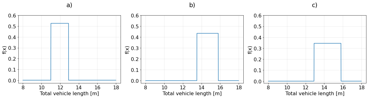
Answer all questions in three decimal places and review the “Waiting time” example questions and answers to help you answer these questions.

Determine whether each statement is TRUE or FALSE

school Campus Bookshelves
menu_book Bookshelves
perm_media Learning Objects
login Login
how_to_reg Request Instructor Account
hub Instructor Commons
Download Page (PDF)
Download Full Book (PDF)
Periodic Table
Physics Constants
Scientific Calculator
Reference & Cite
Tools expand_more
Readability

selected template will load here

This action is not available.

5.20: General Uniform Distributions

Last updated
Save as PDF
Page ID 10360

Kyle Siegrist
University of Alabama in Huntsville via Random Services

This section explores uniform distributions in an abstract setting. If you are a new student of probability, or are not familiar with measure theory, you may want to skip this section and read the sections on the uniform distribution on an interval and the discrete uniform distributions.

Basic Theory

Suppose that $ (S, \mathscr S, \lambda) $ is a measure space. That is, $ S $ is a set, $ \mathscr S $ a $ \sigma $-algebra of subsets of $ S $, and $ \lambda $ a positive measure on $ \mathscr S $. Suppose also that $ 0 \lt \lambda(S) \lt \infty $, so that $ \lambda $ is a finite, positive measure.

Random variable $ X $ with values in $ S $ has the uniform distribution on $ S $ (with respect to $ \lambda $) if \[ \P(X \in A) = \frac{\lambda(A)}{\lambda(S)}, \quad A \in \mathscr S \]

Thus, the probability assigned to a set $ A \in \mathscr S$ depends only on the size of $ A $ (as measured by $ \lambda $).

The most common special cases are as follows:

Discrete : The set $ S $ is finite and non-empty, $ \mathscr S $ is the $ \sigma $-algebra of all subsets of $ S $, and $ \lambda = \# $ (counting measure).
Euclidean : For $n \in \N_+$, let $\mathscr R_n$ denote the $\sigma$-algebra of Borel measureable subsets of $\R^n$ and let $\lambda_n$ denote Lebesgue measure on $(\R^n, \mathscr R_n)$. In this setting, $S \in \mathscr R_n$ with $0 \lt \lambda_n(S) \lt \infty$, $\mathscr S = \{A \in \mathscr R_n: A \subseteq S\}$, and the measure is $\lambda_n$ restricted to $(S, \mathscr S)$.

In the Euclidean case, recall that $ \lambda_1 $ is length measure on $ \R $, $ \lambda_2 $ is area measure on $ \R^2 $, $ \lambda_3 $ is volume measure on $ \R^3 $, and in general $ \lambda_n $ is sometimes referred to as $ n $-dimensional volume. Thus, $ S \in \mathscr R_n $ is a set with positive, finite volume.

Suppose $(S, \mathscr S, \lambda)$ is a finite, positive measure space, as above, and that $ X $ is uniformly distributed on $ S $.

The probability density function $ f $ of $ X $ (with respect to $ \lambda $) is \[ f(x) = \frac{1}{\lambda(S)}, \quad x \in S \]

This follows directly from the definition of probability density function: \[\int_A \frac 1 {\lambda(S)} \, d\lambda(x) = \frac{\lambda(A)}{\lambda(S)}, \quad A \in \mathscr S\]

Thus, the defining property of the uniform distribution on a set is constant density on that set. Another basic property is that uniform distributions are preserved under conditioning.

Suppose that $ R \in \mathscr S $ with $ \lambda(R) \gt 0 $. The conditional distribution of $ X $ given $ X \in R $ is uniform on $ R $.

For $A \in \mathscr S$ with $ A \subseteq R $, \[ \P(X \in A \mid X \in R) = \frac{\P(X \in A)}{\P(X \in R)} = \frac{\lambda(A)/\lambda(S)}{\lambda(R)/\lambda(S)} = \frac{\lambda(A)}{\lambda(R)} \]

In the setting of previous result, suppose that $ \bs{X} = (X_1, X_2, \ldots) $ is a sequence of independent variables, each uniformly distributed on $ S $. Let $ N = \min\{n \in \N_+: X_n \in R\} $. Then $ N $ has the geometric distribution on $ \N_+ $ with success parameter $ p = \P(X \in R) $. More importantly, the distribution of $ X_N $ is the same as the conditional distribution of $ X $ given $ X \in R $, and hence is uniform on $ R $. This is the basis of the rejection method of simulation. If we can simulate a uniform distribution on $ S $, then we can simulate a uniform distribution on $ R $.

If $ h $ is a real-valued function on $ S $, then $ \E[h(X)] $ is the average value of $ h $ on $ S $, as measured by $ \lambda $:

If $ h: S \to \R $ is integrable with respect to $ \lambda $ Then \[ \E[h(X)] = \frac{1}{\lambda(S)} \int_S h(x) \, d\lambda(x) \]

This result follows from the change of variables theorem for expected value, since \[ \E[h(X)] = \int_S h(x) f(x) \, d\lambda(x) = \frac 1 {\lambda(S)} \int_S h(x) \, d\lambda(x)\]

The entropy of the uniform distribution on $ S $ depends only on the size of $ S $, as measured by $ \lambda $:

The entropy of $ X $ is $ H(X) = \ln[\lambda(S)] $.

Product Spaces

Suppose now that $ (S, \mathscr S, \lambda) $ and $ (T, \mathscr T, \mu) $ are finite, positive measure spaces, so that $ 0 \lt \lambda(S) \lt \infty $ and $ 0 \lt \mu(T) \lt \infty $. Recall the product space $ (S \times T, \mathscr S \otimes \mathscr T, \lambda \otimes \mu) $. The product $ \sigma $-algebra $ \mathscr S \otimes \mathscr T $ is the $ \sigma $-algebra of subsets of $ S \times T $ generated by product sets $ A \times B $ where $ A \in \mathscr S $ and $ B \in \mathscr T $. The product measure $ \lambda \otimes \mu $ is the unique positive measure on $ (S \times T, \mathscr S \otimes \mathscr T) $ that satisfies $ (\lambda \otimes \mu)(A \times B) = \lambda(A) \mu(B) $ for $ A \in \mathscr S $ and $ B \in \mathscr T $.

$ (X, Y) $ is uniformly distributed on $ S \times T $ if and only if $ X $ is uniformly distributed on $ S $, $ Y $ is uniformly distributed on $ T $, and $ X $ and $ Y $ are independent.

Suppose first that $ (X, Y) $ is uniformly distributed on $ S \times T$. If $ A \in \mathscr S $ and $ B \in \mathscr T $ then \[ \P(X \in A, Y \in B) = \P[(X, Y) \in A \times B] = \frac{(\lambda \otimes \mu)(A \times B)}{(\lambda \otimes \mu)(S \times T)} = \frac{\lambda(A) \mu(B)}{\lambda(S) \mu(T)} = \frac{\lambda(A)}{\lambda(S)} \frac{\mu(B)}{\mu(T)} \] Taking $ B = T $ in the displayed equation gives $ \P(X \in A) = \lambda(A) \big/ \lambda(S) $ for $ A \in \mathscr S $, so $ X $ is uniformly distributed on $ S $. Taking $ A = S $ in the displayed equation gives $ \P(Y \in B) = \mu(B) \big/ \mu(T) $ for $ B \in \mathscr T $, so $ Y $ is uniformly distributed on $ T $. Returning to the displayed equation generally gives $ \P(X \in A, Y \in B) = \P(X \in A) \P(Y \in B) $ for $ A \in \mathscr S $ and $ B \in \mathscr T $, so $ X $ and $ Y $ are independent.

Conversely, suppose that $ X $ is uniformly distributed on $ S $, $ Y $ is uniformly distributed on $ T $, and $ X $ and $ Y $ are independent. Then for $ A \in \mathscr S $ and $ B \in \mathscr T $, \[ \P[(X, Y) \in A \times B] = \P(X \in A, Y \in B) = \P(X \in A) \P(Y \in B) = \frac{\lambda(A)}{\lambda(S)} \frac{\mu(B)}{\mu(T)} = \frac{\lambda(A) \mu(B)}{\lambda(S) \mu(T)} = \frac{(\lambda \otimes \mu)(A \times B)}{(\lambda \otimes \mu)(S \times T)} \] It then follows (see the section on existence and uniqueness of measures) that $ \P[(X, Y) \in C] = (\lambda \otimes \mu)(C) / (\lambda \otimes \mu)(S \times T) $ for every $ C \in \mathscr S \otimes \mathscr T $, so $ (X, Y) $ is uniformly distributed on $ S \times T $.

www.springer.com The European Mathematical Society

StatProb Collection
Recent changes
Current events
Random page
Project talk
Request account
What links here
Related changes
Special pages
Printable version
Permanent link
Page information
View source

Uniform distribution

2020 Mathematics Subject Classification: Primary: 60E99 [ MSN ][ ZBL ]

A common name for a class of probability distributions, arising as an extension of the idea of "equally possible outcomes" to the continuous case. As with the normal distribution , the uniform distribution appears in probability theory as an exact distribution in some problems and as a limit in others.

1 The uniform distribution on an interval of the line (the rectangular distribution).
2 The uniform distribution on an interval as a limit distribution.
3.1 References

The uniform distribution on an interval of the line (the rectangular distribution).

The uniform distribution on an interval $ [a,\ b] $, $ a < b $, is the probability distribution with density $$ p (x) = \left \{ \begin{array}{ll} { \frac{1}{b - a} } , & x \in [a,\ b], \\ 0, & x \notin [a,\ b]. \\ \end{array} \right .$$ The concept of a uniform distribution on $ [a,\ b] $ corresponds to the representation of a random choice of a point from the interval. The mathematical expectation and variance of the uniform distribution are equal, respectively, to $ (b + a)/2 $ and $ (b - a) ^{2} /12 $. The distribution function is $$ F (x) = \left \{ \begin{array}{ll} 0 , & x \leq a, \\ \frac{x - a}{b - a} , & a < x \leq b, \\ 1, & x > b, \\ \end{array} \right .$$ and the characteristic function is $$ \phi (t) = { \frac{1}{it (b - a)} } (e ^{itb} - e ^{ita} ). $$ A random variable with uniform distribution on $ [0,\ 1] $ can be constructed from a sequence of independent random variables $ X _{1} ,\ X _{2} \dots $ taking the values 0 and 1 with probabilities $ 1/2 $, by putting $$ X = \sum _ {n = 1} ^ \infty X _{n} 2 ^{-n} $$( $ X _{n} $ are the digits in the binary expansion of $ X $). The random number $ X $ has a uniform distribution in the interval $ [0,\ 1] $. This fact has important statistical applications, see, for example, Random and pseudo-random numbers .

If two independent random variables $ X _{1} $ and $ X _{2} $ have uniform distributions on $ [0,\ 1] $, then their sum has the so-called triangular distribution on $ [0,\ 2] $ with density $ u _{2} (x) = 1 - | 1 - x | $ for $ x \in [0,\ 2] $ and $ u _{2} (x) = 0 $ for $ x \notin [0,\ 2] $. The sum of three independent random variables with uniform distributions on $ [0,\ 1] $ has on $ [0,\ 3] $ the distribution with density $$ u _{3} (x) = \left \{ \begin{array}{ll} { \frac{x ^ 2}{2} } , & 0 \leq x < 1, \\ { \frac{[x ^{2} - 3 (x - 1) ^{2} ]}{2} } , & 1 \leq x < 2, \\ { \frac{[x ^{2} - 3 (x - 1) ^{2} + 3 (x - 2) ^{2} ]}{2} } , & 2 \leq x < 3, \\ 0, & x \notin [0,\ 3]. \\ \end{array} \right .$$ In general, the distribution of the sum $ X _{1} + \dots + X _{n} $ of independent variables with uniform distributions on $ [0,\ 1] $ has density $$ u _{n} (x) = { \frac{1}{(n - 1)!} } \sum _ {k = 0} ^ n (-1) ^{k} \binom{n}{k} (x - k) _{+} ^ {n - 1} $$ for $ 0 \leq x \leq n $ and $ u _{n} (x) = 0 $ for $ x \notin [0,\ n] $; here $$ z _{+} = \left \{ \begin{array}{ll} z, & z > 0, \\ 0, & z \leq 0. \\ \end{array} \right .$$ As $ n \rightarrow \infty $, the distribution of the sum $ X _{1} + \dots + X _{n} $, centred around the mathematical expectation $ n/2 $ and scaled by the standard deviation $ \sqrt {n/12} $, tends to the normal distribution with parameters 0 and 1 (the approximation for $ n = 3 $ is already satisfactory for many practical purposes).

In statistical applications the procedure for constructing a random variable $ X $ with given distribution function $ F $ is based on the following fact. Let the random variable $ Y $ be uniformly distributed on $ [0,\ 1] $ and let the distribution function $ F $ be continuous and strictly increasing. Then the random variable $ X = F ^ {\ -1} Y $ has distribution function $ F $( in the general case it is necessary to replace the inverse function $ F ^ {\ -1} (y) $ in the definition of $ X $ by an analogue, namely $ F ^ {\ -1} (y) = \mathop{\rm inf}\nolimits \{ {x} : {F (x) \leq y \leq F (x + 0)} \} $).

The uniform distribution on an interval as a limit distribution.

Some typical examples of the uniform distribution on $ [0,\ 1] $ arising as a limit are given below.

1) Let $ X _{1} ,\ X _{2} \dots $ be independent random variables having the same continuous distribution function. Then the distribution of their sums $ S _{n} $, taken $ \mathop{\rm mod}\nolimits \ 1 $, that is, the distribution of the fractional parts $ \{ S _{n} \} $ of these sums $ S _{n} $, converges to the uniform distribution on $ [0,\ 1] $.

2) Let the random parameters $ \alpha $ and $ \beta $ have an absolutely-continuous joint distribution; then, as $ t \rightarrow \infty $, the distribution of $ \{ \alpha t + \beta \} $ converges to the uniform distribution on $ [0,\ 1] $.

3) A uniform distribution appears as the limit distribution of the fractional parts of certain functions $ g $ on the positive integers. For example, for irrational $ \alpha $ the fraction of those $ m $, $ 1 \leq m \leq n $, for which $$ 0 \leq a \leq \{ na \} \leq b \leq 1, $$ has the limit $ b - a $ as $ n \rightarrow \infty $.

The uniform distribution on subsets of $ \mathbf R ^{k} $.

An example of a uniform distribution in a rectangle appears already in the Buffon problem (see also Geometric probabilities ; Stochastic geometry ). The uniform distribution on a bounded set $ D $ in $ \mathbf R ^{k} $ is defined as the distribution with density $$ p (x _{1} \dots x _{n} ) = \left \{ \begin{array}{ll} C \neq 0, & x \in D, \\ 0, & x \notin D, \\ \end{array} \right .$$ where $ C $ is the inverse of the $ k $- dimensional volume (or Lebesgue measure) of $ D $.

Uniform distributions on surfaces have also been discussed. Thus, a "random direction" (for example, in $ \mathbf R ^{3} $), defined as a vector from the origin to a random point on the surface of the unit sphere, is uniformly distributed in the sense that the probability that it hits a part of the surface is proportional to the area of that part.

The role of the uniform distribution in algebraic groups is played by the normalized Haar measure .

Probability and statistics
Probability theory and stochastic processes
Distribution theory
This page was last edited on 22 December 2019, at 12:00.
Privacy policy
About Encyclopedia of Mathematics
Disclaimers
Impressum-Legal

Home » Histogram – Types, Examples and Making Guide

Histogram – Types, Examples and Making Guide

Table of Contents

Definition:

Histogram is a graphical representation of the distribution of numerical data. It consists of a series of bars, where the height of each bar represents the frequency or relative frequency of the data within a particular interval or “bin.” The intervals, or bins, are typically specified on the x-axis, while the frequency or relative frequency is displayed on the y-axis. Histograms are commonly used in data analysis to visualize the distribution of a dataset, including information about its central tendency, spread, and skewness. They are particularly useful for identifying patterns and outliers in large datasets.

Parts of Histogram

The parts of a histogram include:

The x-axis, or horizontal axis, represents the range of values for the variable being measured. It is divided into intervals or bins, each of which represents a range of values.

The y-axis, or vertical axis, represents the frequency or relative frequency of the data within each interval or bin. The height of each bar represents the frequency or relative frequency of the data within that interval.

The bars in a histogram are vertical rectangles that represent the frequency or relative frequency of the data within each interval or bin. The width of the bars corresponds to the width of the interval or bin.

Intervals or bins

The intervals or bins represent the ranges of values that are grouped together in a histogram. They are typically of equal width and are specified on the x-axis.

The title of the histogram should provide a clear and concise description of the variable being measured and the purpose of the histogram.

If the histogram represents multiple groups or categories, a legend may be included to explain the meaning of each color or pattern used to represent the data.

The shape of the histogram can indicate whether the data is skewed to the left, right, or has a symmetrical distribution. This can be helpful in understanding the distribution of the data and making inferences about the population being measured.

Types of Histogram

Some common types of Histogram are as follows:

Probability Histogram

A probability histogram is a type of histogram that shows the probability density function of a continuous variable. The area under each bar in a probability histogram represents the probability of the data falling within that range.

Bimodal Histogram

A bimodal histogram is a type of histogram that shows two distinct peaks, indicating that the data has two modes or two different populations. Bimodal histograms can indicate that the data is a mixture of two different distributions or that there are two underlying processes contributing to the data.

Uniform Histogram

A uniform histogram is a type of histogram that shows that the data is evenly distributed over a given range. In a uniform histogram, all bars are approximately the same height, indicating that there is an equal probability of the data falling within any given range.

Symmetric Histogram

A symmetric histogram is a type of histogram that shows that the data is evenly distributed around a central value, resulting in a shape that is roughly symmetrical. In a symmetric histogram, the mean, median, and mode are all approximately equal. This means that the distribution of the data is balanced, with roughly the same number of values on either side of the central value. An example of a symmetric histogram is the normal distribution.

How to Make Histogram

Here are the general steps to make a histogram:

Collect and organize the data: Collect the data you want to represent in the histogram. Group the data into intervals or bins, depending on the range and distribution of the data.
Determine the range and interval width: Determine the minimum and maximum values of the data, and decide on an appropriate interval width or bin size. The bin size should be small enough to capture the variability in the data, but large enough to group similar values together.
Draw the horizontal and vertical axes: Draw the horizontal axis and label it with the variable being measured. Draw the vertical axis and label it with the frequency or relative frequency of the data.
Draw the bars : Draw rectangles above each interval or bin, with the height of the rectangle corresponding to the frequency or relative frequency of the data in that bin. The width of the rectangle should be equal to the bin size.
Add titles and labels : Add a title to the histogram that describes the variable being measured and the range of the data. Label the x-axis and y-axis with appropriate units and titles.
Fine-tune the histogram: Adjust the histogram as needed to improve its readability and visual appeal. This may include changing the bin size, adjusting the scale of the axes, or changing the colors and styles of the bars.
Interpret the histogram: Analyze the shape, center, and spread of the data using the histogram. Look for patterns and trends, and draw conclusions based on the data.

Histogram Creating Guide

Here are the steps to create a histogram using a spreadsheet program like Microsoft Excel:

Open a new spreadsheet and enter the data you want to use for the histogram.
Create a column for the bins or intervals you want to use for the histogram. These bins should be evenly spaced and cover the entire range of your data.
Select the data and the bin column, and then click on the “Insert” tab and select “Histogram” from the “Charts” section.
Choose the desired histogram style and format for your chart. You can customize the colors, titles, axis labels, and other chart elements to suit your needs.
Review the histogram and make any necessary adjustments. You may need to adjust the bin size, scale of the axis, or formatting of the bars to make the histogram more informative and visually appealing.
Analyze the histogram and draw conclusions based on the data. Look for patterns, trends, and outliers in the data, and use the histogram to support your analysis and decision-making.

Examples of Histogram

Here are some examples of histograms:

Height of Students in a Class: A histogram of the height of students in a class might show a normal distribution with a peak around the average height of the class.
Daily Temperatures in a City: A histogram of daily temperatures in a city might show a bimodal distribution, with one peak around the average high temperature and another peak around the average low temperature.
Ages of Employees in a Company: A histogram of the ages of employees in a company might show a slightly skewed distribution, with more employees in their 30s and 40s than in their 20s or 50s.
Grades on a Test: A histogram of grades on a test might show a uniform distribution if all the students performed equally well, or a skewed distribution if there are a few high or low scores that are significantly different from the others.
Housing Prices in a Neighborhood: A histogram of housing prices in a neighborhood might show a skewed distribution with a long tail on the high end, indicating that there are a few very expensive houses in the area.

Applications of Histogram

Histograms have many applications in various fields, including:

Quality Control: Histograms are used in quality control to monitor the distribution of product characteristics, such as weight, dimensions, or color. By analyzing histograms, manufacturers can identify and correct problems with production processes and ensure that products meet quality standards.
Market Research: Histograms are used in market research to analyze data on consumer preferences, behavior, and demographics. By analyzing histograms, marketers can identify trends and patterns in consumer data and use this information to develop targeted marketing strategies.
Finance and Economics: Histograms are used in finance and economics to analyze data on stock prices, interest rates, and other financial variables. By analyzing histograms, analysts can identify trends and patterns in financial data and use this information to make investment decisions and develop economic models.
Medical Research: Histograms are used in medical research to analyze data on patient characteristics, such as age, weight, and medical history. By analyzing histograms, researchers can identify risk factors for disease, track the progress of treatment, and identify patterns in health outcomes.
Image Processing: Histograms are used in image processing to analyze and manipulate digital images. By analyzing histograms of image pixels, software can adjust image contrast, brightness, and color balance to enhance image quality and improve visual clarity.

When to use Histogram

They are particularly useful for:

Identifying the shape of a distribution: Histograms can help you identify the shape of a distribution, including whether it is symmetric, skewed, or bimodal.
Identifying central tendency: Histograms can help you identify the center of a distribution, including the mean, median, and mode.
Identifying variability: Histograms can help you identify the range and spread of a distribution, including the minimum and maximum values, as well as the interquartile range and standard deviation.
Identifying outliers: Histograms can help you identify outliers, or extreme values that are significantly different from the rest of the data.
Comparing distributions: Histograms can help you compare the distributions of two or more variables to identify similarities and differences.

Purpose of Histogram

The purpose of a histogram is to visualize the distribution of a dataset. It provides a graphical representation of the frequency or proportion of data points that fall within each interval or bin of a continuous variable. Histograms can reveal patterns and trends in the data that may not be apparent from other methods of analysis, and can help you identify the shape, center, spread, and outliers of a distribution.

Histograms are particularly useful for identifying the following:

The shape of a distribution: Histograms can help you identify whether a distribution is symmetric, skewed, bimodal, or uniform.
The center of a distribution : Histograms can help you identify the mean, median, or mode of a distribution.
The spread of a distribution : Histograms can help you identify the range, interquartile range, or standard deviation of a distribution.
Outliers : Histograms can help you identify values that fall far outside the bulk of the distribution, which may be unusual or extreme.

Advantages of Histogram

Here are some advantages of using a histogram to analyze data:

Easy to interpret: Histograms provide a visual representation of the data that is easy to understand and interpret. The bars in a histogram show the frequency or proportion of data points that fall within each interval or bin, making it easy to see the distribution of the data.
Reveals patterns and trends: Histograms can reveal patterns and trends in the data that may not be apparent from other methods of analysis. By looking at the shape of the distribution, you can identify whether it is symmetric, skewed, bimodal, or uniform, which can provide insights into the underlying data.
Identifies outliers: Histograms can help you identify outliers, or data points that fall far outside the bulk of the distribution. This can be useful for identifying unusual or extreme values that may require further investigation.
Quantitative analysis: Histograms provide a quantitative analysis of the data that can be used to calculate measures such as the mean, median, mode, range, interquartile range, and standard deviation. This can help you gain a more precise understanding of the distribution of the data.
Comparisons: Histograms can be used to compare the distribution of two or more variables, which can reveal similarities and differences in the data.

Limitation of Histogram

Bin size: The shape of the histogram can be affected by the bin size or width, and choosing the appropriate bin size can be subjective. A small bin size can lead to a jagged or noisy histogram, while a large bin size can oversimplify the distribution and obscure important features.
Outliers : Histograms can be affected by outliers, which are data points that fall far outside the bulk of the distribution. Outliers can skew the distribution and make it difficult to interpret the data.
Noisy data: Histograms can be sensitive to noisy or incomplete data, which can affect the shape and interpretation of the distribution.
Subjectivity : The interpretation of histograms can be subjective, and different analysts may choose different bin sizes or interpret the distribution differently.
Limited to one variable: Histograms are limited to analyzing one variable at a time, which can make it difficult to identify relationships between variables.

About the author

Muhammad Hassan

Researcher, Academic Writer, Web developer

Cluster Analysis – Types, Methods and Examples

Discriminant Analysis – Methods, Types and...

MANOVA (Multivariate Analysis of Variance) –...

Documentary Analysis – Methods, Applications and...

ANOVA (Analysis of variance) – Formulas, Types...

Graphical Methods – Types, Examples and Guide

Math Article

Uniform Distribution

What is uniform distribution.

A continuous probability distribution is a Uniform distribution and is related to the events which are equally likely to occur. It is defined by two parameters, x and y, where x = minimum value and y = maximum value. It is generally denoted by u(x, y).

If the probability density function or probability distribution of a uniform distribution with a continuous random variable X is f(b)=1/y-x, then It is denoted by U(x,y), where x and y are constants such that x<a<y. It is written as

X $\begin{array}{l}\sim\end{array} $ U(a,b)

(Note: Check whether the data is inclusive or exclusive before working out problems with uniform distribution.)

Uniform Distribution Examples

Example : The data in the table below are 55 times a baby yawns, in seconds, of a 9-week-old baby girl.

The sample mean = 11.49
The sample standard deviation = 6.23.

As assumed, the yawn times, in secs, it follows a uniform distribution between 0 and 23 seconds(Inclusive).

So, it is equally likely that any yawning time is from 0 to 23.

Histograph Type: Empirical Distribution (It matches with theoretical uniform distribution).

If the length is A, in seconds, of a 9-month-old baby’s yawn.

The uniform distribution notation for the same is A $\begin{array}{l}\sim\end{array} $ U(x,y) where x = the lowest value of a and y = the highest value of b.
f(a) = 1/(y-x), f(a) = the probability density function. For x $\begin{array}{l}\leq\end{array} $ a $\begin{array}{l}\leq\end{array} $ y.

In this example:

X $\begin{array}{l}\sim\end{array} $ U(0,23)

f(a) = 1/(23-0) for 0 $\begin{array}{l}\leq\end{array} $ X $\begin{array}{l}\leq\end{array} $ 23.

Theoretical Mean Formula

Standard deviation formula.

In this example,

The theoretical mean = $\begin{array}{l}\mu\end{array} $ = (x+y)/2

Standard deviation = $\begin{array}{l}\sqrt{ \frac{(23-0)^{2}}{12}}\end{array} $ =6.64 seconds.

Put your understanding of this concept to test by answering a few MCQs. Click ‘Start Quiz’ to begin!

Select the correct answer and click on the “Finish” button Check your score and answers at the end of the quiz

Visit BYJU’S for all Maths related queries and study materials

Your result is as below

Request OTP on Voice Call

Register with BYJU'S & Download Free PDFs

Statistics Made Easy

How to Use the Uniform Distribution in Excel

A uniform distribution is a probability distribution in which every value between an interval from a to b is equally likely to be chosen.

The probability that we will obtain a value between x 1 and x 2 on an interval from a to b can be found using the formula:

P(obtain value between x 1 and x 2 ) = (x 2 – x 1 ) / (b – a)

The uniform distribution has the following properties:

The mean of the distribution is μ = (a + b) / 2
The variance of the distribution is σ 2 = (b – a) 2 / 12
The standard deviation of the distribution is σ = √σ 2

The following examples show how to calculate probabilities for uniform distributions in Excel.

Note: You can double check the solution to each example below using the Uniform Distribution Calculator .

Examples: Uniform Distribution in Excel

Example 1: A bus shows up at a bus stop every 20 minutes. If you arrive at the bus stop, what is the probability that the bus will show up in 8 minutes or less?

a: 0 minutes
b: 20 minutes
x 1 : 0 minutes
x 2 : 8 minutes

The probability that the bus shows up in 8 minutes or less is 0.4 .

Example 2: The weight of a certain species of frog is uniformly distributed between 15 and 25 grams. If you randomly select a frog, what is the probability that the frog weighs between 17 and 19 grams?

a: 15 grams
b: 25 grams
x 1 : 17 grams
x 2 : 19 grams

Probability example with a uniform distribution in Excel

The probability that the frog weighs between 17 and 19 grams is 0.2 .

Example 3: The length of an NBA game is uniformly distributed between 120 and 170 minutes. What is the probability that a randomly selected NBA game lasts more than 150 minutes?

a: 120 minutes
b: 170 minutes
x 1 : 150 minutes
x 2 : 170 minutes

Uniform distribution probabilities in Excel

The probability that a randomly selected NBA game lasts more than 150 minutes is 0.4 .

Find more Excel tutorials on this page .

Featured Posts

Statistics Cheat Sheets to Get Before Your Job Interview

Hey there. My name is Zach Bobbitt. I have a Masters of Science degree in Applied Statistics and I’ve worked on machine learning algorithms for professional businesses in both healthcare and retail. I’m passionate about statistics, machine learning, and data visualization and I created Statology to be a resource for both students and teachers alike. My goal with this site is to help you learn statistics through using simple terms, plenty of real-world examples, and helpful illustrations.

Join the Statology Community

I have read and agree to the terms & conditions

1. Introduction

2. methods and algorithms, 4. software, 5. discussion.

computer programs $\def\hfill{\hskip 5em}\def\hfil{\hskip 3em}\def\eqno#1{\hfil {#1}}$

Program VUE : analysing distributions of cryo-EM projections using uniform spherical grids

a Architecture et Réactivité de l'ARN, UPR 9002 CNRS, IBMC, Université de Strasbourg, 15 rue R. Descartes, 67084 Strasbourg, France, b Centre for Integrative Biology (CBI), Department of Integrated Structural Biology, IGBMC (Institute of Genetics and of Molecular and Cellular Biology), Centre National de la Recherche Scientifique (CNRS) UMR 7104, Institut National de la Santé de la Recherche Médicale (Inserm) U964, Université de Strasbourg, 1 rue Laurent Fries, 67404 Illkirch, France, and c Université de Lorraine, Physics Department, 54506 Vandoeuvre-lès-Nancy, France * Correspondence e-mail: [email protected]

Three-dimensional cryo electron microscopy reconstructions are obtained by extracting information from a large number of projections of the object. These projections correspond to different `views' or `orientations', i.e. directions in which these projections show the reconstructed object. Uneven distribution of these views and the presence of dominating preferred orientations may distort the reconstructed spatial images. This work describes the program VUE (views on uniform grids for cryo electron microscopy), designed to study such distributions. Its algorithms, based on uniform virtual grids on a sphere, allow an easy calculation and accurate quantitative analysis of the frequency distribution of the views. The key computational element is the Lambert azimuthal equal-area projection of a spherical uniform grid onto a disc. This projection keeps the surface area constant and represents the frequency distribution with no visual bias. Since it has multiple tunable parameters, the program is easily adaptable to individual needs, and to the features of a particular project or of the figure to be produced. It can help identify problems related to an uneven distribution of views. Optionally, it can modify the list of projections, distributing the views more uniformly. The program can also be used as a teaching tool.

Keywords: 3D reconstruction ; cryo-EM ; view frequency ; preferred orientations ; uniform grids ; Lambert projection .

In cryo electron microscopy (cryo-EM), three-dimensional (3D) reconstructions are obtained from two-dimensional (2D) projections of the object. There are two priors to achieve correct results:

(i) The object is unique and structurally homogeneous, otherwise classifications and structure sorting are required.

(ii) The orientations of the object corresponding to the projections are evenly distributed in space, otherwise the frequency of occurrence of the same or close orientations should be considered.

(i) How to calculate the frequency of different projections, also known as orientations.

(ii) How to express this information, in particular that about over- and under-represented orientations, accurately and in an efficient way.

(iii) How to use this information to analyse possible deformations of the 3D reconstruction and eventually to improve the latter.

In this work, we address the two first questions. A practical answer to the third question is a separate project for which the tools discussed in this article can be used.

The frequency of views can be expressed numerically in several different ways:

(i) Calculate how much each particular view is separated from other views.

(ii) Calculate how many different views are close to each other and how close.

(iii) Calculate how often a given or similar view is represented in the list of views.

The methods and algorithms of both frequency calculation and its mapping as realized in the different programs are documented rather poorly, probably being considered as auxiliary and technical. Another common weak point is that, when printing maps of distributions calculated as described above or drawing a non-interactive 2D projection of the presentation as bars on the spherical surface, these images represent information rather qualitatively, distorting the relative area of the spherical surface regions.

Selecting appropriate algorithms among these multiple options, we have developed the program VUE to calculate the frequencies of views (of 2D projections), to quantify and visualize their distributions by a plane image, and eventually to produce a new set of views distributed more uniformly. Working on this project, we addressed several goals:

(i) Develop a stand-alone tool which can provide various types of information about the distribution of projections, in both numeric and graphical forms.

(ii) Make the graphical representation quantitatively correct , i.e. such that the area of the 2D regions in the plane image is proportional to the area that they cover on the spherical surface.

(iii) Describe explicitly and in detail the methods and algorithms used for the computations, making them reproducible if required.

(iv) Propose multiple choices of options for different steps of the procedure, allowing the user to produce images adapted to their personal taste in terms of details, colours etc. and to analyse the role of different parameters .

(v) Make this program composed of small modules, allowing one to routinely add other options if required.

(vi) Prepare a tool to analyse, in a separate project, the role of weighting schemes optimizing the 3D reconstruction.

In particular, this program may be considered not only as a research and illustrative tool but also as a methodological and training one.

2.1. Geometric tools

2.1.1. coordinate systems, rotations and views, 2.1.2. lambert projection, 2.2. uniform grids.

A uniform grid on a sphere is a grid such that all its cells have equal, or near equal, surface area. Because the Lambert projection conserves the surface area, it is possible to build first a uniform grid on a disc, which is a simpler task, and then to project it onto the sphere. The current version of the program can use two uniform grids described below. Both of them are constructed starting from concentric circles on a disc and are easy to manipulate.

2.3. Calculation of the views' frequencies

2.3.1. point representation of a view, 2.3.2. symmetries.

For symmetric objects, a statistical analysis may be distorted in two opposing ways. On one hand, the presence of views covering only a part of the sphere may allow a full representation of all views and recovery of all Fourier coefficients equally well. However, a statistical analysis of the formally present views will indicate a highly uneven distribution with large empty regions. On the other hand, the available views may result in a non-uniform covering of the sphere if considering all their symmetry-related copies.

2.3.3. Histogram calculation

In order to compare the total contribution

2.3.4. Frequencies of individual views

2.4. weighting of views.

Other weighting schemes can be implemented routinely.

2.5. Updating of views

The choice of correction mode and of its parameters depends on the 3D reconstruction method. Comparison of the weighting and view processing schemes based on frequency, weights and eventually on other types of information will be discussed elsewhere.

3.1. Data used

Uniform grids make it routine to extract different types of information, to calculate various kinds of statistics and to express it in different forms. This includes both images and a numeric output, as discussed below. To illustrate the options of the program, several experimental data sets measured for the human ribosome have been used.

3.2. Frequency map

By default, the axis of the Lambert projection coincides with the beam direction. This can be reassigned by the user, and the views will be recalculated and shown for the respective hemisphere following the new chosen direction.

3.3. Distribution of individual views

3.4. histograms, 3.5. ribosome, extended data set, 3.6. ribosome, reduced set, 3.7. ribosome, data set set3, 4.1. program overview.

The algorithms discussed above have been realized in the stand-alone program VUE (views on uniform grids for cryo electron microscopy) written in Python3. The program requires a file of parameters with the standard name VUE.dat and a file with the parameters of the projections. The name of this file is defined in VUE.dat and this is the only mandatory parameter. A large list of optional parameters allows the user to adjust the program routinely to their goals and taste, and to the features of the data set and of the project. The program creates up to four diagrams, a text file VUE.log and, by request, an output file with the modified list of views.

4.2. Input file of projections

4.3. plotted maps and histograms.

The program can plot both the view frequency distribution on a hemisphere, presenting it as a map in the Lambert projection, and the distribution of individual views, also in the same projection. Both diagrams are optional and can be selected by the input data of the program; these data can also define the parameters of the diagrams. The direction of the Lambert projection, which by default follows the OZ axis, can be changed to any other defined by its spherical angles, e.g. after being estimated using the superimposable coarse reference grid.

The histograms are also optional. As mentioned previously, their argument values are taken on a logarithmic scale in base two.

4.4. Numeric information

When running, the program traces its progress on the command-line screen.

The output text file VUE.log mirrors the program parameters, especially their modified values and the values of the view histogram, and contains principal statistical information about the data.

If required, the program creates an output file in the same format as the input file. The records of the input file, describing the views, may be completed by the frequency of a given view and the weight calculated according to the chosen scheme. These records can also be either randomly removed, in the case of their over-representation, or multiplied according to the chosen scheme, so that the output file contains the views distributed more uniformly than initially.

For test goals and a rapid check of the set of views by a subsequent express 3D reconstruction, the program can randomly and uniformly select a given part, as defined by the user.

4.5. Program parameters

The program is highly adaptable to individual preferences, both for calculation and for the results presentation. The full list of optional parameters, with the default and allowed values and comments, is given in the file VUE_example.dat . This includes the choice of the type of diagrams to be prepared, the grid type and its size, the frequency calculation parameters, the weighting and colour schemes, the colour bar size, the dot size for individual views, the symmetry operators, the parameters of the eventual view set correction, and many others.

Some auxiliary parameters, for example those defining the position and size of labels on the plots, titles etc. , cannot be modified using keywords but are accessible and commented at the top of the Python script and therefore can be modified from there.

4.6. System and software requirements

Calculation and plotting of the frequency map with the number of projections of the order of 10 5 to 10 6 and with the grid number M = 90 recommended for accurate illustrations takes about a minute or less on an ordinary laptop computer. When the number of views approaches 10 6 , drawing the map of individual views becomes the most time-consuming step (this time is independent of the grid size). However, as discussed above, representing this distribution for so large a number of views may not be a good choice.

The program, the file VUE_example.dat and some test data are available on request from the authors or from the web sites https://git.cbi.igbmc.fr/sacha/vue-cryo-em-software and https://ibmc.cnrs.fr/en/laboratoire/arn-en/presentation/structures-software-and-websites/ .

The developed program VUE gives a practical example of such frequency analysis using these tools. This program, available as stand-alone Python-based software, can be easily adapted to the features of different projects and data. It can be routinely integrated into other packages as a whole or by its components.

The output program information, in both numeric and graphic formats, can be used for a qualitative analysis of the data and indication of eventual problems, as well as for illustrations in publications. A more advanced goal is to use these data to improve the image distortions and artefacts caused by correcting the distribution of views. The program proposes several options for such correction. Comparison of weighting schemes and details of processes to correct the sets of views are separate projects beyond this program description.

Technical details of uniform grids

This grid recalls a grid built in Cartesian axes with easy identification of the neighbouring cells. Its disadvantage is a particular treatment of the cells on diagonals.

Acknowledgements

We thank L. Fréchin for help with the experimental data, M. Schatz, O. von Loeffelholz and anonymous reviewers for useful advice, and the Integral Structural Biology platform at CBI/IGBMC and Informatics Service for support.

Funding information

This work was supported by CNRS, Institut National du Cancer (INCa_16099), the Fondation pour la Recherche Médicale (FRM and FDT202304016898), Agence Nationale pour la Recherche (ANR), the French Infrastructure for Integrated Structural Biology (FRISBI) (ANR-10-INSB-05-01), Instruct-ERIC, iNEXT-Discovery and the ITI 2021–2028 programme of the University of Strasbourg with IdEx Unistra (ANR-10-IDEX-0002), SFRI-STRAT'US (ANR 20-SFRI-0012) and EUR IMCBio (ANR-17-EURE-0023) under the framework of the France 2030 programme.

This is an open-access article distributed under the terms of the Creative Commons Attribution (CC-BY) Licence , which permits unrestricted use, distribution, and reproduction in any medium, provided the original authors and source are cited.

IMAGES

Types Of Graph Representation In Data Structure
Symmetric Distribution in Statistics
Uniform Distribution in Statistics: Definition & Examples
Illustrative example showing that uniformly distributed draws on a unit
Representation of the domain [0 , 1] × [0 , 1] by uniformly distributed
How To Draw Graphs Graphical Representation Of Data S

VIDEO

Functional and Graphical representation of infinite range Discrete Time Signals
Definition-pdf and Distribution Function of Rectangular or Uniform Distribution
Graphical representation of uniformly accelerated motion
Graphical Representation Of Data
Univariate Distributions
What is a distributed representation? #ai #machinelearning #technology

COMMENTS

Uniform Distribution: Definition & Examples
Below, I'll graph discrete and continuous forms of the distribution. For discrete uniform distributions, finding the probability for each outcome is 1/n, where n is the number of outcomes. Rolling dice has six outcomes that are uniformly distributed. Therefore, each one has a likelihood of 1/6 = 0.167. The bar chart below displays the ...
5.3: The Uniform Distribution
Figure 5.3.3. Uniform Distribution between 1.5 and four with shaded area between two and four representing the probability that the repair time x is greater than two. b. P(x < 3) = (base)(height) = (3- 1.5)(0.4) = 0.6. The graph of the rectangle showing the entire distribution would remain the same.
Continuous uniform distribution
In a graphical representation of the continuous uniform distribution function [()], the area under the curve within the specified bounds, displaying the probability, is a rectangle. For the specific example above, the base would be 16 , {\displaystyle 16,} and the height would be 1 23 . {\displaystyle {\tfrac {1}{23}}.}
6.3: The Uniform Distribution
The total duration of baseball games in the major league in the 2011 season is uniformly distributed between 447 hours and 521 hours inclusive. ... The graph of the rectangle showing the entire distribution would remain the same. However the graph should be shaded between $x = 1.5$ and $x = 3$. ...
The Uniform Distribution
The graph of the rectangle showing the entire distribution would remain the same. However the graph should be shaded between x = 1.5 and x = 3. Note that the shaded area starts at x = 1.5 rather than at x = 0; since X ~ U (1.5, 4), x can not be less than 1.5.
The Uniform Distribution
Uniform Distribution between 1.5 and four with shaded area between two and four representing the probability that the repair time x is greater than two; P(x < 3) = (base)(height) = (3 - 1.5)(0.4) = 0.6The graph of the rectangle showing the entire distribution would remain the same. However the graph should be shaded between x = 1.5 and x = 3.
Uniform distribution
The uniform distribution is characterized as follows. Definition Let be a continuous random variable. Let its support be a closed interval of real numbers: We say that has a uniform distribution on the interval if and only if its probability density function is. A random variable having a uniform distribution is also called a uniform random ...
5.2 The Uniform Distribution
The amount of time a service technician needs to change the oil in a car is uniformly distributed between 11 and 21 minutes. Let X = the time needed to change the oil on a car. Write the random variable X in words. X = _____. Write the distribution. Graph the distribution. Find P (x > 19). Find the 50 th percentile.
4.3: Uniform Distributions
Definition 4.3.1 4.3. 1. A random variable X X has a uniform distribution on interval [a, b] [ a, b], write X ∼ uniform[a, b] X ∼ uniform [ a, b], if it has pdf given by. f(x) = { 1 b−a, 0, for a ≤ x ≤ b otherwise f ( x) = { 1 b − a, for a ≤ x ≤ b 0, otherwise. The uniform distribution is also sometimes referred to as the box ...
Uniform distribution
The uniform distribution is the simplest type of continuous probability distribution. The uniform distribution for a continuous random variable is defined by a constant probability density over an interval [a,b]. The probability density function (PDF) of the continuous uniform distribution is: f ( x) = { 1 b − a for a ≤ x ≤ b, 0 for x < a ...
Uniform Distribution
A uniform distribution is a probability distribution in statistics where every outcome is equally likely. There are two types of uniform distribution: discrete uniform distribution. continuous ...
5.20: General Uniform Distributions
Suppose (S, S, λ) is a finite, positive measure space, as above, and that X is uniformly distributed on S. The probability density function f of X (with respect to λ) is f(x) = 1 λ(S), x ∈ S. Proof. Thus, the defining property of the uniform distribution on a set is constant density on that set. Another basic property is that uniform ...
Uniform distribution
Uniform distributions on surfaces have also been discussed. Thus, a "random direction" (for example, in $ \mathbf R ^{3} $), defined as a vector from the origin to a random point on the surface of the unit sphere, is uniformly distributed in the sense that the probability that it hits a part of the surface is proportional to the area of that part.
Uniform Histogram
Definition: A uniform histogram is a type of histogram where all the bins (or categories) have the same frequency or count. In other words, the distribution of values across the different bins is even or uniform. This means that each bin represents an equal range of values, and the histogram appears as a rectangular shape.
PDF Gaussian Graphical Models
Gaussian Graphical Models. We then write X Nd( ; ). Hence is the mean vector and the covariance matrix of the distribution. The de nition (1) makes sense if and only if > 0, i.e. if is positive semide nite. Note that we have allowed distributions with variance zero. and let t = 1, = > , and 2 = > .
Histogram
A uniform histogram is a type of histogram that shows that the data is evenly distributed over a given range. In a uniform histogram, all bars are approximately the same height, indicating that there is an equal probability of the data falling within any given range. ... It provides a graphical representation of the frequency or proportion of ...
What is Uniform Distribution?, Its Examples and Formulas
A continuous probability distribution is a Uniform distribution and is related to the events which are equally likely to occur. It is defined by two parameters, x and y, where x = minimum value and y = maximum value. It is generally denoted by u (x, y). OR. If the probability density function or probability distribution of a uniform ...
How to Use the Uniform Distribution in Excel
The probability that we will obtain a value between x1 and x2 on an interval from a to b can be found using the formula: P (obtain value between x1 and x2) = (x2 - x1) / (b - a) The uniform distribution has the following properties: The mean of the distribution is μ = (a + b) / 2. The variance of the distribution is σ2 = (b - a)2 / 12.
Uniform Distribution
Graph functions, plot points, visualize algebraic equations, add sliders, animate graphs, and more. Uniform Distribution - Area Under the Curve. Save Copy. Log InorSign Up. f x = 1 2 0 1. ∫ b 1 2 0 f x dx. 2. b = 1 4 0. 3. 0 ≤ y ≤ f x 1 2 0 < x < b. 4. 5. powered by. powered by ...
Classifying shapes of distributions (video)
Meanwhile, a random distribution, if graphed, will look uniform. Because it is random, then any given data point will have an equal chance of landing in each bucket. For example, rolling the dice will yield a roughly uniform distribution graph because each time you roll the die, each number is equally likely to come up.
Learning invariant and uniformly distributed feature space for multi
A representation learning method for multi-view generation is proposed. • The proposed multi-view representations are view-invariant and uniformly-distributed. • We design our generation model based on the contrastive framework. • Experimental results demonstrate the superiority of the proposed method.
PDF arXiv:2311.13953v1 [cs.LG] 23 Nov 2023
ACOT. ACOT aims to exploit the cluster predictions of both original graph representations and augmented graph representations to discover reliable and uniformly distributed pseudo labels. Our inspiration of ACOT comes from self-labeling [21] which extends standard cross-entropy minimization to an optimal transport (OT) problem [22]. In this way ...
(IUCr) Program VUE: analysing distributions of cryo-EM projections
(ii) Make the graphical representation quantitatively correct, ... so that the output file contains the views distributed more uniformly than initially. For test goals and a rapid check of the set of views by a subsequent express 3D reconstruction, the program can randomly and uniformly select a given part, as defined by the user. ...

6.3: The Uniform Distribution

Chapter Review

Formula Review

Contributors

The Uniform Distribution

Chapter Review

Formula Review

Module 5: Continuous Random Variables

Concept Review

Formula Review

Expected value

How to cite

5.2 The Uniform Distribution

Example 5.2

Example 5.3

Example 5.4

Example 5.5

Example 5.6

Uniform distribution

2. Waiting time #

3. Total vehicle length #

5.20: General Uniform Distributions

Basic Theory

Product Spaces

Uniform distribution

The uniform distribution on an interval of the line (the rectangular distribution).

The uniform distribution on an interval as a limit distribution.

The uniform distribution on subsets of $ \mathbf R ^{k} $.

Histogram – Types, Examples and Making Guide

Parts of Histogram

Intervals or bins

Types of Histogram

Probability Histogram

Bimodal Histogram

Uniform Histogram

Symmetric Histogram

How to Make Histogram

Histogram Creating Guide

Examples of Histogram

Applications of Histogram

When to use Histogram

Purpose of Histogram

Advantages of Histogram

Limitation of Histogram

About the author

Muhammad Hassan

You may also like

Cluster Analysis – Types, Methods and Examples

Discriminant Analysis – Methods, Types and...

MANOVA (Multivariate Analysis of Variance) –...

Documentary Analysis – Methods, Applications and...

ANOVA (Analysis of variance) – Formulas, Types...

Graphical Methods – Types, Examples and Guide

Uniform Distribution

Uniform Distribution Examples

Theoretical Mean Formula

Leave a Comment Cancel reply

Register with BYJU'S & Download Free PDFs

How to Use the Uniform Distribution in Excel

Examples: Uniform Distribution in Excel

Featured Posts

Leave a Reply Cancel reply

Join the Statology Community

1. Introduction

computer programs \(\def\hfill{\hskip 5em}\def\hfil{\hskip 3em}\def\eqno#1{\hfil {#1}}\)

Program VUE : analysing distributions of cryo-EM projections using uniform spherical grids

2.1. Geometric tools

2.3. Calculation of the views' frequencies

2.3.3. Histogram calculation

2.3.4. Frequencies of individual views

2.5. Updating of views

3.1. Data used

3.2. Frequency map

3.3. Distribution of individual views

4.2. Input file of projections

4.4. Numeric information

4.5. Program parameters

4.6. System and software requirements

Technical details of uniform grids

Acknowledgements