assignment model as a particular case of transportation model

Integrating activity-based and traffic assignment models: Methodology and case study application

Ieee account.

Change Username/Password
Update Address

Purchase Details

Payment Options
Order History
View Purchased Documents

Profile Information

Communications Preferences
Profession and Education
Technical Interests
US & Canada: +1 800 678 4333
Worldwide: +1 732 981 0060
Contact & Support
About IEEE Xplore
Accessibility
Terms of Use
Nondiscrimination Policy
Privacy & Opting Out of Cookies

A not-for-profit organization, IEEE is the world's largest technical professional organization dedicated to advancing technology for the benefit of humanity. © Copyright 2024 IEEE - All rights reserved. Use of this web site signifies your agreement to the terms and conditions.

Architecture and Design
Asian and Pacific Studies
Business and Economics
Classical and Ancient Near Eastern Studies
Computer Sciences
Cultural Studies
Engineering
General Interest
Geosciences
Industrial Chemistry
Islamic and Middle Eastern Studies
Jewish Studies
Library and Information Science, Book Studies
Life Sciences
Linguistics and Semiotics
Literary Studies
Materials Sciences
Mathematics
Social Sciences
Sports and Recreation
Theology and Religion
Publish your article
The role of authors
Promoting your article
Abstracting & indexing
Publishing Ethics
Why publish with De Gruyter
How to publish with De Gruyter
Our book series
Our subject areas
Your digital product at De Gruyter
Contribute to our reference works
Product information
Tools & resources
Product Information
Promotional Materials
Orders and Inquiries
FAQ for Library Suppliers and Book Sellers
Repository Policy
Free access policy
Open Access agreements
Database portals
For Authors
Customer service
People + Culture
Journal Management
How to join us
Working at De Gruyter
Mission & Vision
De Gruyter Foundation
De Gruyter Ebound
Our Responsibility
Partner publishers

Your purchase has been completed. Your documents are now available to view.

Chapter 5: Transportation, Assignment, and Network Models

From the book managerial decision modeling.

Nagraj (Raju) Balakrishnan , Barry Render , Ralph Stair and Chuck Munson
X / Twitter

Supplementary Materials

Please login or register with De Gruyter to order this product.

Chapters in this book (21)

The Assignment Model

The linear programming formulation of the assignment model is similar to the formulation of the transportation model, except all the supply values for each source equal one, and all the demand values at each destination equal one. Thus, our example is formulated as follows :

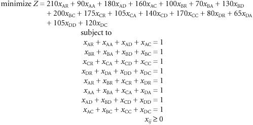
assignment model as a particular case of transportation model

This is a balanced assignment model. An unbalanced model exists when supply exceeds demand or demand exceeds supply.

What Security Is and Isnt
Process for Assessing Risk
Risk Assessment Best Practices
Putting Together a Toolkit
Recommendations
Overview of JDBC Resources
Container-Managed Relationships
Load-Balancing Schemes
Creating an Identity Assertion Provider
Implementing the Backend Components
Miscellaneous Solutions
Storage and Maintenance of CDR Data
Infrastructure Solutions
Application Solutions
Working with Microsoft Visual Studio .NET 2003 and Microsoft .NET Framework 1.1
Building Web Applications
Interacting with the Operating System
Windows Server 2003 for .NET Developers
ASP.NET Core Server Controls
Real-World Data Access
The HTTP Request Context
HTTP Handlers and Modules
Storing Web Data in an SQL Database
Installing SOAP Libraries
Listing the Newsgroups on a Server
Running Commands on a Remote Server
Managing Multiple Services

MBA Knowledge Base

Business • Management • Technology

Home » Management Science » Transportation and Assignment Models in Operations Research

Transportation and Assignment Models in Operations Research

Transportation and assignment models are special purpose algorithms of the linear programming. The simplex method of Linear Programming Problems(LPP) proves to be inefficient is certain situations like determining optimum assignment of jobs to persons, supply of materials from several supply points to several destinations and the like. More effective solution models have been evolved and these are called assignment and transportation models.

The transportation model is concerned with selecting the routes between supply and demand points in order to minimize costs of transportation subject to constraints of supply at any supply point and demand at any demand point. Assume a company has 4 manufacturing plants with different capacity levels, and 5 regional distribution centres. 4 x 5 = 20 routes are possible. Given the transportation costs per load of each of 20 routes between the manufacturing (supply) plants and the regional distribution (demand) centres, and supply and demand constraints, how many loads can be transported through different routes so as to minimize transportation costs? The answer to this question is obtained easily through the transportation algorithm.

Similarly, how are we to assign different jobs to different persons/machines, given cost of job completion for each pair of job machine/person? The objective is minimizing total cost. This is best solved through assignment algorithm.

Uses of Transportation and Assignment Models in Decision Making

The broad purposes of Transportation and Assignment models in LPP are just mentioned above. Now we have just enumerated the different situations where we can make use of these models.

Transportation model is used in the following:

To decide the transportation of new materials from various centres to different manufacturing plants. In the case of multi-plant company this is highly useful.
To decide the transportation of finished goods from different manufacturing plants to the different distribution centres. For a multi-plant-multi-market company this is useful.
To decide the transportation of finished goods from different manufacturing plants to the different distribution centres. For a multi-plant-multi-market company this is useful. These two are the uses of transportation model. The objective is minimizing transportation cost.

Assignment model is used in the following:

To decide the assignment of jobs to persons/machines, the assignment model is used.
To decide the route a traveling executive has to adopt (dealing with the order inn which he/she has to visit different places).
To decide the order in which different activities performed on one and the same facility be taken up.

In the case of transportation model, the supply quantity may be less or more than the demand. Similarly the assignment model, the number of jobs may be equal to, less or more than the number of machines/persons available. In all these cases the simplex method of LPP can be adopted, but transportation and assignment models are more effective, less time consuming and easier than the LPP.

Operations Research approach of problem solving
Introduction to Transportation Problem
Procedure for finding an optimum solution for transportation problem
Initial basic feasible solution of a transportation problem
Top 7 Best Ways of Getting MBA Assignment Writing Help
Introduction to Decision Models
Transportation Cost Elements
Modes of Transportation in Logistics
Factors Affecting Transportation in Logistics
Export/Import Transportation Systems

One thought on “ Transportation and Assignment Models in Operations Research ”

Exclussive dff. And easy understude

Transportation and Assignment Models

The linear programs in Chapters 1 and 2 are all examples of classical ''activity'' models. In such models the variables and constraints deal with distinctly different kinds of activities-tons of steel produced versus hours of mill time used, or packages of food bought versus percentages of nutrients supplied. To use these models you must supply coefficients like tons per hour or percentages per package that convert a unit of activity in the variables to the corresponding amount of activity in the constraints. This chapter addresses a significantly different but equally common kind of model, in which something is shipped or assigned, but not converted. The resulting constraints, which reflect both limitations on availability and requirements for delivery, have an especially simple form. We begin by describing the so-called transportation problem, in which a single good is to be shipped from several origins to several destinations at minimum overall cost. This problem gives rise to the simplest kind of linear program for minimum-cost flows. We then generalize to a transportation model, an essential step if we are to manage all the data, variables and constraints effectively. As with the diet model, the power of the transportation model lies in its adaptability. We continue by considering some other interpretations of the ''flow'' from origins to destinations, and work through one particular interpretation in which the variables represent assignments rather than shipments. The transportation model is only the most elementary kind of minimum-cost flow model. More general models are often best expressed as networks, in which nodes-some of which may be origins or destinations-are connected by arcs that carry flows of some kind. AMPL offers convenient features for describing network flow models, including node and arc declarations that specify network structure directly. Network models and the relevant AMPL features are the topic of Chapter 15. 43

Related Papers

sachin gupta

Models of networks have appeared in several chapters, notably in the transportation problems in Chapter 3. We now return to the formulation of these models, and AMPL's features for handling them. Figure 15-1 shows the sort of diagram commonly used to describe a network problem. A circle represents a node of the network, and an arrow denotes an arc running from one node to another. A flow of some kind travels from node to node along the arcs, in the directions of the arrows. An endless variety of models involve optimization over such networks. Many cannot be expressed in any straightforward algebraic way or are very difficult to solve. Our discussion starts with a particular class of network optimization models in which the decision variables represent the amounts of flow on the arcs, and the constraints are limited to two kinds: simple bounds on the flows, and conservation of flow at the nodes. Models restricted in this way give rise to the problems known as network linear programs. They are especially easy to describe and solve, yet are widely applicable. Some of their benefits extend to certain generalizations of the network flow form, which we also touch upon. We begin with minimum-cost transshipment models, which are the largest and most intuitive source of network linear programs, and then proceed to other well-known cases: maximum flow, shortest path, transportation and assignment models. Examples are initially given in terms of standard AMPL variables and constraints, defined in var and subject to declarations. In later sections, we introduce node and arc declarations that permit models to be described more directly in terms of their network structure. The last section discusses formulating network models so that the resulting linear programs can be solved most efficiently. 15.1 Minimum-cost transshipment models As a concrete example, imagine that the nodes and arcs in Figure 15-1 represent cities and intercity transportation links. A manufacturing plant at the city marked PITT will

books.google.com

Robert Fourer

Transportation Research Part B: Methodological

M. Grazia Speranza

Diego Klabjan

The Transportation Problem is the special class of Linear Programming Problem. It arises when the situation in which a commodity is shipped from sources to destinations. The main object is to determine the amounts shipped from each sources to each destinations which minimize the total shipping cost while satisfying both supply criteria and demand requirements. In this paper, we are giving the idea about to finding the Initial Basic Feasible solution as well as the optimal solution or near to the optimal solution of a Transportation problem using the method known as " An Alternate Approach to find an optimal Solution of a Transportation Problem ". An Algorithm provided here, concentrate at unoccupied cells and proceeds further. Also, the numerical examples are provided to explain the proposed algorithm. However, the above method gives a step by step development of the solution procedure for finding an optimal solution.

Mollah Mesbahuddin Ahmed

Industries require planning in transporting their products from production centres to the users end with minimal transporting cost to maximize profit. This process is known as Transportation Problem which is used to analyze and minimize transportation cost. This problem is well discussed in operation research for its wide application in various fields, such as scheduling, personnel assignment, product mix problems and many others, so that this problem is really not confined to transportation or distribution only. In the solution procedure of a transportation problem, finding an initial basic feasible solution is the prerequisite to obtain the optimal solution. Again, development is a continuous and endless process to find the best among the bests. The growing complexity of management calls for development of sound methods and techniques for solution of the problems. Considering these factors, this research aims to propose an algorithm " Incessant Allocation Method " to obtain an initial basic feasible solution for the transportation problems. Several numbers of numerical problems are also solved to justify the method. Obtained results show that the proposed algorithm is effective in solving transportation problems.

IRJET Journal

Augmented Reality is an advanced technology that could simplify the execution of complex operations. Augmented reality(AR) describes the real-world interaction where digital information is superimposed in the real world environment with additional information. This concept can be used for online shopping to enhance the user experience.

RECIMA21 - Revista Científica Multidisciplinar - ISSN 2675-6218

Enir Fonseca

O sistema educacional foi fortemente impactado nos anos de 2020 e 2021 com classificação pela OMS de pandemia o surto de COVID-19, impossibilitando reuniões em salas de aulas e do contato físico. Os gestores buscaram soluções para superar estas adversidades, proporcionando aos docentes, mecanismos que permitissem atender as necessidades acadêmicas e manutenção da qualidade do ensino. A solução imediata para estes obstáculos, só foi possível graças a evolução e disponibilidade das TDICs. Para consecução deste trabalho, que tem como principal objetivo, investigar a partir do feedback discente, o aprendizado nas aulas construídas no ambiente Teams, realizamos uma pesquisa exploratória, com a coleta de dados no formulário Forms, realizadas no segundo semestre de 2020 e primeiro semestre de 2021, com entrevistas realizadas nas aulas presenciais ocorridas no segundo semestre de 2021. As principais conclusões indicam que a evolução das TDICs possibilitou uma rápida transição e adequação do...

International Journal of Hydrogen Energy

Isabel J Ferrer

9 Introduction to Transportation Modeling: Travel Demand Modeling and Data Collection

Chapter overview.

Chapter 9 serves as an introduction to travel demand modeling, a crucial aspect of transportation planning and policy analysis. As explained in previous chapters, the spatial distribution of activities such as employment centers, residential areas, and transportation systems mutually influence each other. The utilization of travel demand forecasting techniques leads to dynamic processes in urban areas. A comprehensive grasp of travel demand modeling is imperative for individuals involved in transportation planning and implementation.

This chapter covers the fundamentals of the traditional four-step travel demand modeling approach. It delves into the necessary procedures for applying the model, including establishing goals and criteria, defining scenarios, developing alternatives, collecting data, and conducting forecasting and evaluation.

Following this chapter, each of the four steps will be discussed in detail in Chapters 10 through 13.

Learning Objectives

Describe the need for travel demand modeling in urban transportation and relate it to the structure of the four-step model (FSM).
Summarize each step of FSM and the prerequisites for each in terms of data requirement and model calibration.
Summarize the available methods for each of the first three steps of FSM and compare their reliability.
Identify assumptions and limitations of each of the four steps and ways to improve the model.

Introduction

Transportation planning and policy analysis heavily rely on travel demand modeling to assess different policy scenarios and inform decision-making processes. Throughout our discussion, we have primarily explored the connection between urban activities, represented as land uses, and travel demands, represented by improvements and interventions in transportation infrastructure. Figure 9.1 provides a humorous yet insightful depiction of the transportation modeling process. In preceding chapters, we have delved into the relationship between land use and transportation systems, with the houses and factories in the figure symbolizing two crucial inputs into the transportation model: households and jobs. The output of this model comprises transportation plans, encompassing infrastructure enhancements and programs. Chapter 9 delves into a specific model—travel demand modeling. For further insights into transportation planning and programming, readers are encouraged to consult the UTA OERtransport book, “Transportation Planning, Policies, and History.”

A graphical representation of FSM input and outputs data in the process.

Travel demand models forecast how people will travel by processing thousands of individual travel decisions. These decisions are influenced by various factors, including living arrangements, the characteristics of the individual making the trip, available destination options, and choices regarding route and mode of transportation. Mathematical relationships are used to represent human behavior in these decisions based on existing data.

Through a sequential process, transportation modeling provides forecasts to address questions such as:

What will the future of the area look like?
What is the estimated population for the forecasting year?
How are job opportunities distributed by type and category?
What are the anticipated travel patterns in the future?
How many trips will people make? ( Trip Generation )
Where will these trips end? ( Trip Distribution )
Which transportation mode will be utilized? ( Mode Split )
What will be the demand for different corridors, highways, and streets? ( Traffic Assignment )
Lastly, what impact will this modeled travel demand have on our area? (Rahman, 2008).

9.2 Four-step Model

According to the questions above, Transportation modeling consists of two main stages, regarding the questions outlined above. Firstly, addressing the initial four questions involves demographic and land use analysis, which incorporates the community vision collected through citizen engagement and input. Secondly, the process moves on to the four-step travel demand modeling (FSM), which addresses questions 5 through 8. While FSM is generally accurate for aggregate calculations, it may occasionally falter in providing a reliable test for policy scenarios. The limitations of this model will be explored further in this chapter.

In the first stage, we develop an understanding of the study area from demographic information and urban form (land-use distribution pattern). These are important for all the reasons we discussed in this book. For instance, we must obtain the current age structure of the study area, based on which we can forecast future birth rates, death, and migrations (Beimborn & Kennedy, 1996).

Regarding economic forecasts, we must identify existing and future employment centers since they are the basis of work travel, shopping travel, or other travel purposes. Empirically speaking, employment often grows as the population grows, and the migration rate also depends on a region’s economic growth. A region should be able to generate new employment while sustaining the existing ones based upon past trends and form the basis for judgment for future trends (Mladenovic & Trifunovic, 2014).

After forecasting future population and employment, we must predict where people go (work, shop, school, or other locations). Land-use maps and plans are used in this stage to identify the activity concentrations in the study area. Future urban growth and land use can follow the same trend or change due to several factors, such as the availability of open land for development and local plans and zoning ordinances (Beimborn & Kennedy, 1996). Figure 9.3 shows different possible land-use patterns frequently seen in American cities.

This pictures shows 6 different land use patterns that are: (a) traditional grid, (b) post-war suburb, (c) traditional neighborhood design, (d) fused grid, (e) post-war suburb II, and (f) tranditional neighborhood design II.

Land-use pattern can also be forecasted through the integration of land use and transportation as we explored in previous chapters.

Figure 9.3 above shows a simple structure of the second stage of FSM.

This picture shows the sequence of the fours steps of FSM.

Once the number and types of trips are predicted, they are assigned to various destinations and modes. In the final step, these trips are allocated to the transportation network to compute the total demand for each road segment. During this second stage, additional choices such as the time of travel and whether to travel at all can be modeled using choice models (McNally, 2007). Travel forecasting involves simulating human behavior through mathematical series and calculations, capturing the sequence of decisions individuals make within an urban environment.

The first attempt at this type of analysis in the U.S. occurred during the post-war development period, driven by rapid economic growth. The influential study by Mitchell and Rapkin (1954) emphasized the need to establish a connection between travel and activities, highlighting the necessity for a comprehensive framework. Initial development models for trip generation, distribution, and diversion emerged in the 1950s, leading to the application of the four-step travel demand modeling (FSM) approach in a transportation study in the Chicago area. This model was primarily highway-oriented, aiming to compare new facility development and improved traffic engineering. In the 1960s, federal legislation mandated comprehensive and continuous transportation planning, formalizing the use of FSM. During the 1970s, scholars recognized the need to revise the model to address emerging concerns such as environmental issues and the rise of multimodal transportation systems. Consequently, enhancements were made, leading to the development of disaggregate travel demand forecasting and equilibrium assignment methods that complemented FSM. Today, FSM has been instrumental in forecasting travel demand for over 50 years (McNally, 2007; Weiner, 1997).

Initially outlined by Mannheim (1979), the basic structure of FSM was later expanded by Florian, Gaudry, and Lardinois (1988). Figure 9.3 illustrates various influential components of travel demand modeling. In this representation, “T” represents transportation, encompassing all elements related to the transportation system and its services. “A” denotes the activity system, defined according to land-use patterns and socio-demographic conditions. “P” refers to transportation network performance. “D,” which stands for demand, is generated based on the land-use pattern. According to Florian, Gaudry, and Lardinois (1988), “L” and “S” (location and supply procedures) are optional parts of FSM and are rarely integrated into the model.

This flowchart shows the relationship between various components of transportation network and their joint impact on traffic volume (flow) on the network.

A crucial aspect of the process involves understanding the input units, which are defined both spatially and temporally. Demand generates person trips, which encompass both time and space (e.g., person trips per household or peak-hour person trips per zone). Performance typically yields a level of service, defined as a link volume capacity ratio (e.g., freeway vehicle trips per hour or boardings per hour for a specific transit route segment). Demand is primarily defined at the zonal level, whereas performance is evaluated at the link level.

It is essential to recognize that travel forecasting models like FSM are continuous processes. Model generation takes time, and changes may occur in the study area during the analysis period.

Before proceeding with the four steps of FSM, defining the study area is crucial. Like most models discussed, FSM uses traffic analysis zones (TAZs) as the geographic unit of analysis. However, a higher number of TAZs generally yield more accurate results. The number of TAZs in the model can vary based on its purpose, data availability, and vintage. These zones are characterized or categorized by factors such as population and employment. For modeling simplicity, FSM assumes that trip-making begins at the center of a zone (zone centroid) and excludes very short trips that start and end within a TAZ, such as those made by bike or on foot.

Furthermore, highway systems and transit systems are considered as networks in the model. Highway or transit line segments are coded as links, while intersections are represented as nodes. Data regarding network conditions, including travel times, speeds, capacity, and directions, are utilized in the travel simulation process. Trips originate from trip generation zones, traverse a network of links and nodes, and conclude at trip attraction zones.

Trip Generation

Trip generation is the first step in the FSM model. This step defines the magnitude of daily travel in the study area for different trip purposes. It will also provide us with an estimate of the total trips to and from each zone, creating a trip production and attraction matrix for each trip’s purpose. Trip purposes are typically categorized as follows:

Home-based work trips (work trips that begin or end at home),
Home-based shopping trips,
Home-based other trips,
School trips,
Non-home-based trips (trips that neitherbeginnorendathome),
Trucktrips,and
Taxitrips(Ahmed,2012).

Trip attractions are based on the level of employment in a zone. In the trip generation step, the assumptions and limitations are listed below:

Independent decisions: Travel behavior is affected by many factors generated within a household; the model ignores most of these factors. For example, childcare may force people to change their travel plans.
Limited trip purposes: This model consists of a limited number of trip purposes for simplicity, giving rise to some model limitations. Take shopping trips, for example; they are all considered in the same weather conditions. Similarly, we generate home-based trips for various purposes (banking, visiting friends, medical reasons, or other purposes), all of which are affected by factors ignored by the model.
Trip combinations: Travelers are often willing to combine various trips into a chain of short trips. While this behavior creates a complex process, the FSM model treats this complexity in a limited way.
Feedback, cause, and effect problems: Trip generation often uses factors that are a function of the number of trips. For instance, for shopping trip attractions in the FSM model, we assume they are a retail employment function. However, it is logical to assume how many customers these retail centers attract. Alternatively, we can assume that the number of trips a household makes is affected by the number of private cars they own. Nevertheless, the activity levels of families determine the total number of cars.

As mentioned, trip generation process estimations are done separately for each trip purpose. Equations 1 and 2 show the function of trip generation and attraction:

$O_i = f(x_{i1}, x_{i2}, x_{i3}, \ldots)$

where Oi and Dj trip are generated and attracted respectively, x refers to socio-economic characteristics, and y refers to land-use properties.

Generally, FSM aggregates different trip purposes previously listed into three categories: home-based work trips (HBW) , home-based other (or non-work) trips (HBO) , and non-home-based trips (NHB) . Trip ends are either the origin (generation) or destination (attraction), and home-end trips comprise most trips in a study area. We can also model trips at different levels, such as zones, households, or person levels (activity-based models). Household-level models are the most common scale for trip productions, and zonal-level models are appropriate for trip attractions (McNally, 2007).

There are three main methods for a trip generation or attraction.

The first method is multiple regression based on population, jobs, and income variables.
The second method in this step is experience-based analysis, which can show us the ratio of trips generated frequently.
The third method is cross-classification . Cross-classification is like the experience-based analysis in that it uses trip rates but in an extended format for different categories of trips (home-based trips or non-home-based trips) and different attributes of households, such as car ownership or income.

Elaborating on the differences between these methods, category analysis models are more common for the trip generation model, while regression models demonstrate better performance for trip attractions (Meyer, 2016). Production models are recognized to be influenced by a range of explanatory and policy-sensitive variables (e.g., car ownership, household income, household size, and the number of workers). However, estimation is more problematic for attraction models because regional travel surveys are at the household level (thus providing more accurate data for production models) and not for nonresidential land uses (which is important for trip attraction). Additionally, estimation can be problematic because explanatory trip attraction variables may usually underperform (McNally, 2007). For these reasons, survey data factoring is required prior to relating sample trips to population-level attraction variables, typically achieved via regression analysis. Table 9.1 shows the advantages and disadvantages of each of these two models.

Trip Distribution

Thus far, the number of trips beginning or ending in a particular zone have been calculated. The second step explores how trips are distributed between zones and how many trips are exchanged between two zones. Imagine a shopping trip. There are multiple options for accessible shopping malls accessible. However, in the end, only one will be selected for the destination. This information is modeled in the second step as a distribution of trips. The second step results are usually a very large Origin-Destination (O-D) matrix for each trip purpose. The O-D matrix can look like the table below (9.2), in which sum of Tij by j shows us the total number of trips attracted in zone J and the sum of Tij by I yield the total number of trips produced in zone I.

Up to this point, we have calculated the number of trips originating from or terminating in a specific zone. The next step involves examining how these trips are distributed across different zones and how many trips are exchanged between pairs of zones. To illustrate, consider a shopping trip: there are various options for reaching shopping malls, but ultimately, only one option is chosen as the destination. This process is modeled in the second step as the distribution of trips. The outcome of this step typically yields a large Origin-Destination (O-D) matrix for each trip purpose. An O-D matrix might resemble the table below (9.2), where the sum of Tij by j indicates the total number of trips attracted to zone J, and the sum of Tij by I represents the total number of trips originating from zone I.

$T_{ij} = \frac{P(A_i F_{ij}(K_{ij}))}{\sum(A_x F_{ij}(k_{ix}))}$

T ij = trips produced at I and attracted at j

P i = total trip production at I

A j = total trip attraction at j

F ij = a calibration term for interchange ij , (friction factor) or travel

time factor ( F ij =C/t ij n )

C= calibration factor for the friction factor

K ij = a socioeconomic adjustment factor for interchange ij

i = origin zone

n = number of zones

Different methods (units) in the gravity model can be used to perform distance measurements. For instance, distance can be represented by time, network distance, or travel costs. For travel costs, auto travel cost is the most common and straightforward way of monetizing distance. A combination of different costs, such as travel time, toll payments, parking payments, etc., can also be used. Alternatively, a composite cost of both car and transit costs can be used (McNally, 2007).

Generalized travel costs can be a function of time divided into different segments. For instance, public transit time can be divided into the following segments: in-vehicle time, walking time, waiting time, interchange time, fare, etc. Since travelers perceive time value differently for each segment (like in-vehicle time vs. waiting time), weights are assigned based on the perceived value of time (VOT). Similarly, car travel costs can be categorized into in-vehicle travel time or distance, parking charge, tolls, etc.

As with the first step in the FSM model, the second step has assumptions and limitations that are briefly explained below.

Constant trip times: In order to utilize the model for prediction, it assumes that the duration of trips remains constant. This means that travel distances are measured by travel time, and the assumption is that enhancements in the transportation system, which reduce travel times, are counterbalanced by the separation of origins and destinations.
Automobile travel times to represent distance: We utilize travel time as a proxy for travel distance. In the gravity model, this primarily relies on private car travel time and excludes travel times via other modes like public transit. This leads to a broader distribution of trips.
Limited consideration of socio-economic and cultural factors: Another drawback of the gravity model is its neglect of certain socio-economic or cultural factors. Essentially, this model relies on trip production and attraction rates along with travel times between them for predictions. Consequently, it may overestimate trip rates between high-income groups and nearby low-income Traffic Analysis Zones (TAZs). Therefore, incorporating more socio-economic factors into the model would enhance accuracy.
Feedback issues: The gravity model’s reliance on travel times is heavily influenced by congestion levels on roads. However, measuring congestion proves challenging, as discussed in subsequent sections. Typically, travel times are initially assumed and later verified. If the assumed values deviate from actual values, they require adjustment, and the calculations need to be rerun.

Mode choice

FSM model’s third step is a mode-choice estimation that helps identify what types of transportation travelers use for different trip purposes to offer information about users’ travel behavior. This usually results in generating the share of each transportation mode (in percentages) from the total number of trips in a study area using the utility function (Ahmed, 2012). Performing mode-choice estimations is crucial as it determines the relative attractiveness and usage of various transportation modes, such as public transit, carpooling, or private cars. Modal split analysis helps evaluate improvement programs or proposals (e.g., congestion pricing or parking charges) aimed at enhancing accessibility or service levels. It is essential to identify the factors contributing to the utility and disutility of different modes for different travel demands (Beimborn & Kennedy, 1996). Comparing the disutility of different modes between two points aids in determining mode share. Disutility typically refers to the burdens of making a trip, such as time, costs (fuel, parking, tolls, etc.). Once disutility is modeled for different trip purposes between two points, trips can be assigned to various modes based on their utility. As discussed in Chapter 12, a mode’s advantage in terms of utility over another can result in a higher share of trips using that mode.

The assumptions and limitations for this step are outlined as follows:

Choices are only affected by travel time and cost: This model assumes that changes in mode choices occur solely if transportation cost or travel time in the transportation network or transit system is altered. For instance, a more convenient transit mode with the same travel time and cost does not affect the model’s results.
Omitted factors: Certain factors like crime, safety, and security, which are not included in the model, are assumed to have no effect, despite being considered in the calibration process. However, modes with different attributes regarding these omitted factors yield no difference in the results.
Simplified access times: The model typically overlooks factors related to the quality of access, such as neighborhood safety, walkability, and weather conditions. Consequently, considerations like walkability and the impact of a bike-sharing program on the attractiveness of different modes are not factored into the model.
Constant weights: The model assumes that the significance of travel time and cost remains constant for all trip purposes. However, given the diverse nature of trip purposes, travelers may prioritize travel time and cost differently depending on the purpose of their trip.

The most common framework for mode choice models is the nested logit model, which can accommodate various explanatory variables. However, before the final step, results need to be aggregated for each zone (Koppelman & Bhat, 2006).

A generalized modal split chart is depicted in Figure 9.5.

a simple decision tree for transportation mode choice between car, train, and walking.

In our analysis, we can use binary logit models (dummy variable for dependent variable) if we have two modes of transportation (like private cars and public transit only). A binary logit model in the FSM model shows us if changes in travel costs would occur, such as what portion of trips changes by a specific mode of transport. The mathematical form of this model is:

$P_ij^1=\frac{T_ij^1}{T_{ij}}\ =\frac{e^-bcij^1 }{e^(-bc_ij^1 )+e^(-bc_ij^2 )}$

where: P_ij 1= The proportion of trips between i and j by mode 1 . Tij 1= Trips between i and j by mode 1.

Cij 1= Generalized cost of travel between i and j by mode 1 .

Cij^2= Generalized cost of travel between i and j by mode 2 .

b= Dispersion Parameter measuring sensitivity to cost.

It is also possible to have a hierarchy of transportation modes for using a binary logit model. For instance, we can first conduct the analysis for the private car and public transit and then use the result of public transit to conduct a binary analysis between rail and bus.

Trip assignment

After breaking down trip counts by mode of transportation, we analyze the routes commuters take from their starting point to their destination, especially for private car trips. This process is known as trip assignment and is the most intricate stage within the FSM model. Initially, the minimum path assigns trips for each origin-destination pair based on either travel costs or time. Subsequently, the assigned volume of trips is compared to the capacity of the route to determine if congestion would occur. If congestion does happen (meaning that traffic volume exceeds capacity), the speed of the route needs to be decreased, resulting in increased travel costs or time. When the Volume/Capacity ratio (v/c ratio) changes due to congestion, it can lead to alterations in both speed and the shortest path. This characteristic of the model necessitates an iterative process until equilibrium is achieved.

The process for public transit is similar, but with one distinction: instead of adjusting travel times, headways are adjusted. Headway refers to the time between successive arrivals of a vehicle at a stop. The duration of headways directly impacts the capacity and volume for each transit vehicle. Understanding the concept of equilibrium in the trip assignment step is crucial because it guides the iterative process of the model. The conclusion of this process is marked by equilibrium, a concept known as Wardrop equilibrium. In Wardrop equilibrium, traffic naturally organizes itself in congested networks so that individual commuters do not switch routes to reduce travel time or costs. Additionally, another crucial factor in this step is the time of day.

Like previous steps, the following assumptions and limitations are pertinent to the trip assignment step:

1. Delays on links: Most traffic assignment models assume that delays occur on the links, not the intersections. For highways with extensive intersections, this can be problematic because intersections involve highly complex movements. Intersections are excessively simplified if the assignment process does not modify control systems to reach an equilibrium.

2. Points and links are only for trips: This model assumes that all trips begin and finish at a single point in a zone (centroids), and commuters only use the links considered in the model network. However, these points and links can vary in the real world, and other arterials or streets might be used for commutes.

3. Roadway capacities: In this model, a simple assumption helps determine roadways’ capacity. Capacity is found based on the number of lanes a roadway provides and the type of road (highway or arterial).

4. Time of the day variations: Traffic volume varies greatly throughout the day and week. In this model, a typical workday of the week is considered and converted to peak hour conditions. A factor used for this step is called the hour adjustment factor. This value is critical because a small number can result in a massive difference in the congestion level forecasted on the model.

5. Emphasis on peak hour travel: The model forecasts for the peak hour but does not forecast for the rest of the day. The models make forecasts for a typical weekday but neglect specific conditions of that time of the year. After completing the fourth step, precise approximations of travel demand or traffic count on each road are achieved. Further models can be used to simulate transportation’s negative or positive externalities. These externalities include air pollution, updated travel times, delays, congestion, car accidents, toll revenues, etc. These need independent models such as emission rate models (Beimborn & Kennedy, 1996).

The basic equilibrium condition point calculation is an algorithm that involves the computation of minimum paths using an all-or-nothing (AON) assignment model to these paths. However, to reach equilibrium, multiple iterations are needed. In AON, it is assumed that the network is empty, and a free flow is possible. The first iteration of the AON assignment requires loading the traffic by finding the shortest path. Due to congestion and delayed travel times, the

previous shortest paths may no longer be the best minimum path for a pair of O-D. If we observe a notable decrease in travel time or cost in subsequent iterations, then it means the equilibrium point has not been reached, and we must continue the estimation. Typically, the following factors affect private car travel times: distance, free flow speed on links, link capacity, link speed capacity, and speed flow relationship .

The relationship between the traffic flow and travel time equation used in the fourth step is:

$t = t_0 + a v^n, \quad v < c$

t= link travel time per length unit

t 0 =free-flow travel time

v=link flow

c=link capacity

a, b, and n are model (calibrated) parameters

Model improvement

Improvements to FSM continue to generate more accurate results. Since transportation dynamics in urban and regional areas are under the complex influence of various factors, the existing models may not be able to incorporate all of them. These can be employer-based trip reduction programs, walking and biking improvement schemes, a shift in departure (time of the day), or more detailed information on socio-demographic and land-use-related factors. However, incorporating some of these variables is difficult and can require minor or even significant modifications to the model and/or computational capacities or software improvements. The following section identifies some areas believed to improve the FSM model performance and accuracy.

• Better data: An effective way of improving the model accuracy is to gather a complete dataset that represents the general characteristics of the population and travel pattern. If the data is out- of-date or incomplete, we will get poor results.

• Better modal split: As you saw in previous sections, the only modes incorporated into the model are private car and public transit trips, while in some cities, a considerable fraction of trips are made by bicycle or by walking. We can improve our models by producing methods to consider these trips in the first and third steps.

• Auto occupancy: In contemporary transportation planning practices, especially in the US, some new policies are emerging for carpooling. We can calculate auto occupancy rates using different mode types, such as carpooling, sensitive to private car trips’ disutility, parking costs, or introducing a new HOV lane.

• Time of the day: In this chapter, the FSM framework discussed is oriented toward peak hour (single time of the day) travel patterns. Nonetheless, understanding the nature of congestion in other hours of the day is also helpful for understanding how travelers choose their travel time.

• A broader trip purpose: Additional trip purposes may provide a better understanding of the

factors affecting different trip purposes and trip-chaining behaviors. We can improve accuracy by having more trip purposes (more disaggregate input and output for the model).

The concept of access: As discussed, land-use policies that encourage public transit use or create amenities for more convenient walking are not present in the model. Developing factors or indices that reflect such improvements in areas with high demand for non-private vehicles and incorporating them in choice models can be a good improvement.
Land use feedback: To better understand interactions between land use and travel demand, a land-use simulation model can be added to these steps to determine how a proposed transportation change will lead to a change in land use.
Intersection delays: As mentioned in the fourth step, intersections in major highways create significant delays. Incorporating models that calculate delays at these intersections, such as stop signs, could be another improvement to the model.

A Simple Example of the FSM model

An example of FSM is provided in this section to illustrate a typical application of this model in the U.S. In the first phase, the specifications about the transportation network and household data are needed. In this hypothetical example, 5 percent of households in each TAZ were sampled and surveyed, which generated 1,955 trips in 200 households. As a hypothetical case study, this sample falls below the standard required for statistical significance but is relevant to demonstrate FSM.

A home interview survey was carried out to gather data from a five percent sample of households in each TAZ. This survey resulted in 1,852 trips from 200 households. It is important to note that the sample size in this example falls below the minimum required for statistical significance, as it is intended for learning purposes only.

Table 9.3 provides network information such as speed limits, number of lanes, and capacity. Table 9.4 displays the total number of households and jobs in three industry sectors for each zone. Additionally, Table 9.5 breaks down the household data into three car ownership groups, which is one of the most significant factors influencing trip making.

In the first step (trip generation), a category model (i.e., cross-classification) helped estimate trips. The sampled population’s sociodemographic and trip data for different purposes helped calculate this estimate. Since research has shown the significant effect of auto ownership on private car trip- making (Ben-Akiva & Lerman, 1974), disaggregating the population based on the number of private cars generates accurate results. Table 9.7 shows the trip-making rate for different income and auto ownership groups.

Also, as mentioned in previous sections, multiple regression estimation analysis can be used to generate the results for the attraction model. Table 9.7 shows the equations for each of the trip purposes.

After estimating production and attraction, the models are used for population data to generate results for the first step. Next, comparing the results of trip production and attraction, we can observe that the total number of trips for each purpose is different. This can be due to using different methods for production and attraction. Since the production method is more reliable, attraction is typically normalized by production. Also, some external zones in our study area are either attracting trips from our zones or generating them. In this case, another alternative is to extend the boundary of the study area and include more zones.

As mentioned, the total number of trips produced and attracted are different in these results. To address this mismatch, we can use a balance factor to come up with the same trip generation and attraction numbers if we want to keep the number of zones within our study area. Alternatively, we can consider some external stations in addition to designated zones. In this example, using the latter seems more rational because, as we saw in Table 9.4, there are more jobs than the number of households aggregately, and our zone may attract trips from external locations.

For the trip distribution step, we use the gravity model. For internal trips, the gravity model is:

$T_{ij} = a_i b_j P_i A_j f(t_{ij})$

and f(tij) is some function of network level of service (LOS)

To apply the gravity model, we need to calculate the impedance function first, which is represented here by travel cost. Table 9.9 shows the minimum travel path between each pair of zones ( skim tree ) in a matrix format in which each cell represents travel time required to travel between the corresponding row and column of that cell.

Table 9.9-Travel cost table (skim tree)

Note. Table adapted from “The Four-Step Model” by M. McNally, In D. A. Hensher, & K. J. Button (Eds.), Handbook of transport modelling , Volume1, p. 5, Bingley, UK: Emerald Publishing. Copyright 2007 by Emerald Publishing.

With having minimum travel costs between each pair of zones, we can calculate the impedance function for each trip purpose using the formula

$f(t_{ij}) = a \cdot t_{ij} \cdot b \cdot e^{ct_{ij}}$

Table 9.10 shows the model parameters for calculating the impedance function for different trip purposes:

After calculating the impedance function , we can calculate the result of the trip distribution. This stage generates trip matrices since we calculate trips between each zone pair. These matrices are usually in “Origin-Destination” (OD) format and can be disaggregated by the time of day. Field surveys help us develop a base-year trip distribution for different periods and trip purposes. Later, these empirical results will help forecast trip distribution. When processing the surveys, the proportion of trips from the production zone to the attraction zone (P-A) is also generated. This example can be seen in Table 9.11. Looking at a specific example, the first row in table is for the 2-hour morning peak commute time period. The table documents that the production to attraction factor for the home-based work trip is 0.3. Unsurprisingly, the opposite direction, attraction to production zone is 0.0 for this time of day. Additionally, the table shows that the factor for HBO and NHB trips are low but do occur during this time period. This could represent shopping trips or trips to school. Table 9.11 table also contains the information for average occupancy levels of vehicles from surveys. This information can be used to convert person trips to vehicle trips or vice versa.

Table 9.11 Trip distribution rates for different time of the day and trip purposes

The O-D trip table is calculated by adding the multiplication of the P-to-A factor by corresponding cell of the P-A trip table and adding the corresponding cell of the transposed P-A trip table multiplied by the A-to-P factor. These results, which are the final output of second step, are shown in Table 9.12.

Once the Production-Attraction (P-A) table is transformed into Origin-Destination (O-D) format and the complete O-D matrix is computed, the outcomes will be aggregated for mode choice and traffic assignment modeling. Further elaboration on these two steps will be provided in Chapters 11 and 12.

In this chapter, we provided a comprehensive yet concise overview of four-step travel demand modeling including the process, the interrelationships and input data, modeling part and extraction of outputs. The complex nature of cities and regions in terms of travel behavior, the connection to the built environment and constantly growing nature of urban landscape, necessitate building models that are able to forecast travel patterns for better anticipate and prepare for future conditions from multiple perspectives such as environmental preservation, equitable distribution of benefits, safety, or efficiency planning. As we explored in this book, nearly all the land-use/transportation models embed a transportation demand module or sub model for translating magnitude of activities and interconnections into travel demand such as VMT, ridership, congestion, toll usage, etc. Four-step models can be categorized as gravity-based, equilibrium-based models from the traditional approaches. To improve these models, several new extensions has been developed such as simultaneous mode and destination choice, multimodality (more options for mode choice with utility), or microsimulation models that improve granularity of models by representing individuals or agents rather than zones or neighborhoods.

Travel demand modeling are models that predicts the flow of traffic or travel demand between zones in a city using a sequence of steps.

Intermodality refers to the concept of utilizing two or more travel modes for a trip such as biking to a transit station and riding the light rail.
Multimodality is a type of transportation network in which a variety of modes such as public transit, rail, biking networks, etc. are offered.

Zoning ordinances is legal categorization of land use policies that permits or prohibits certain built environment factors such as density.

Volume capacity ratio is ratio that divides the demand on a link by the capacity to determine the level of service.

Zone centroid is usually the geometric center of a zone in modeling process where all trips originate and end.

Home-based work trips (HBW) are the trips that originates from home location to work location usually in the AM peak.

Home-based other (or non-work) trips (HBO) are the trips that originates from home to destinations other than work like shopping or leisure.

Non-home-based trips (NHB) are the trips that neither origin nor the destination are home or they are part of a linked trip.

Cross-classification is a method for trip production estimation that disaggregates trip rates in an extended format for different categories of trips like home-based trips or non-home-based trips and different attributes of households such as car ownership or income.

Generalized travel costs is a function of time divided into sections such as in vehicle time vs. waiting time or transfer time in a transit trip.

Binary logit models is a type of logit model where the dependent variable can take only a value of 0 or 1.

Wardrop equilibrium is a state in traffic assignment model where are drivers are reluctant to change their path because the average travel time is at a minimum.

All-or-nothing (AON) assignment model is a model that assumes all trips between two zones uses the shortest path regardless of volume.

Speed flow relationship is a function that determines the speed based on the volume (flow)

skim tree is structure of travel time by defining minimum cost path for each section of a trip.

Key Takeaways

In this chapter, we covered:

What travel demand modeling is for and what the common methods are to do that.
How FSM is structured sequentially, what the relationships between different steps are, and what the outputs are.
What the advantages and disadvantages of different methods and assumptions in each step are.
What certain data collection and preparation for trip generation and distribution are needed through a hypothetical example.

Prep/quiz/assessments

What is the need for regular travel demand forecasting, and what are its two major components?
Describe what data we require for each of the four steps.
What are the advantages and disadvantages of regression and cross-classification methods for a trip generation?
What is the most common modeling framework for mode choice, and what result will it provide us?
What are the main limitations of FSM, and how can they be addressed? Describe the need for travel demand modeling in urban transportation and relate it to the structure of the four-step model (FSM).

Ahmed, B. (2012). The traditional four steps transportation modeling using a simplified transport network: A case study of Dhaka City, Bangladesh. International Journal of Advanced Scientific Engineering and Technological Research , 1 (1), 19–40. https://discovery.ucl.ac.uk/id/eprint/1418961/

ALMEC, C . (2015). The Project for capacity development on transportation planning and database management in the republic of the Philippines: MMUTIS update and enhancement project (MUCEP) : Project Completion Report . Japan International Cooperation Agency. (JICA) Department of Transportation and Communications (DOTC) . https://books.google.com/books?id=VajqswEACAAJ .

Beimborn, E., and Kennedy, R. (1996). Inside the black box: Making transportation models work for livable communities . Washington, DC: Citizens for a Better Environment and the Environmental Defense Fund. https://www.piercecountywa.gov/DocumentCenter/View/755/A-GuideToModeling?bidId

Ben-Akiva, M., & Lerman, S. R. (1974). Some estimation results of a simultaneous model of auto ownership and mode choice to work. Transportation , 3 (4), 357–376. https://doi.org/10.1007/bf00167966

Ewing, R., & Cervero, R. (2010). Travel and the built environment: A meta-analysis. Journal of the American Planning Association , 76 (3), 265–294. https://doi.org/10.1080/01944361003766766

Florian, M., Gaudry, M., & Lardinois, C. (1988). A two-dimensional framework for the understanding of transportation planning models. Transportation Research Part B: Methodological , 22 (6), 411–419. https://doi.org/10.1016/0191-2615(88)90022-7

Hadi, M., Ozen, H., & Shabanian, S. (2012). Use of dynamic traffic assignment in FSUTMS in support of transportation planning in Florida. Florida International University Lehman Center for Transportation Research. https://rosap.ntl.bts.gov/view/dot/24925

Hansen, W. (1959). How accessibility shapes land use.” Journal of the American Institute of Planners 25 (2): 73–76. https://doi.org/10.1080/01944365908978307

Gavu, E. K. (2010). Network based indicators for prioritising the location of a new urban transport connection: Case study Istanbul, Turkey (Master’s thesis, University of Twente). International Institute for Geo-Information Science and Earth Observation Enschede. http://essay.utwente.nl/90752/1/Emmanuel%20Kofi%20Gavu-22239.pdf

Karner, A., London, J., Rowangould, D., & Manaugh, K. (2020). From transportation equity to transportation justice: Within, through, and beyond the state. Journal of Planning Literature , 35 (4), 440–459. https://doi.org/10.1177/0885412220927691

Kneebone, E., & Berube, A. (2013). Confronting suburban poverty in America . Brookings Institution Press.

Koppelman, Frank S, and Chandra Bhat. (2006). A self instructing course in mode choice modeling: multinomial and nested logit models. U.S. Department of Transportation Federal Transit Administration https://www.caee.utexas.edu/prof/bhat/COURSES/LM_Draft_060131Final-060630.pdf

‌Manheim, M. L. (1979). Fundamentals of transportation systems analysis. Volume 1: Basic Concepts . The MIT Press https://mitpress.mit.edu/9780262632898/fundamentals-of-transportation-systems-analysis/

McNally, M. G. (2007). The four step model. In D. A. Hensher, & K. J. Button (Eds.), Handbook of transport modelling , Volume1 (pp.35–53). Bingley, UK: Emerald Publishing.

Meyer, M. D., & Institute Of Transportation Engineers. (2016). Transportation planning handbook . Wiley.

Mladenovic, M., & Trifunovic, A. (2014). The shortcomings of the conventional four step travel demand forecasting process. Journal of Road and Traffic Engineering , 60 (1), 5–12.

Mitchell, R. B., and C. Rapkin. (1954). Urban traffic: A function of land use . Columbia University Press. https://doi.org/10.7312/mitc94522

Rahman, M. S. (2008). “ Understanding the linkages of travel behavior with socioeconomic characteristics and spatial Environments in Dhaka City and urban transport policy applications .” Hiroshima: (Master’s thesis, Hiroshima University.) Graduate School for International Development and Cooperation. http://sr-milan.tripod.com/Master_Thesis.pdf

Rodrigue, J., Comtois, C., & Slack, B. (2020). The geography of transport systems . London ; New York Routledge.

Shen, Q. (1998). Location characteristics of inner-city neighborhoods and employment accessibility of low-wage workers. Environment and Planning B: Planning and Design , 25 (3), 345–365.

Sharifiasl, S., Kharel, S., & Pan, Q. (2023). Incorporating job competition and matching to an indicator-based transportation equity analysis for auto and transit in Dallas-Fort Worth Area. Transportation Research Record , 03611981231167424. https://doi.org/10.1177/03611981231167424

Weiner, Edward. 1997. Urban transportation planning in the United States: An historical overview . US Department of Transportation. https://rosap.ntl.bts.gov/view/dot/13691

Xiongbing, J, Grammenos, F. (2013, May, 21) . Taking the Guesswork out of Designing for Walkability. Planetizen . https://www.planetizen.com/node/63248

Home-based other (or non-work) trips (HBO) are the trips that originates from home to destinations other than work like shopping or leisure.

gravity model is a type of accessibility measurement in which the employment in destination and population in the origin defines thee degree of accessibility between the two zones.

Impedance function is a function that convert travel costs (usually time or distance) to the level of difficulty of getting from one location to the other.

Share This Book

Models for Traffic Assignment to Transportation Networks

Cite this chapter.

Ennio Cascetta 3

Part of the book series: Applied Optimization ((APOP,volume 49))

1074 Accesses

2 Citations

Models for traffic assignment to transportation networks simulate how demand and supply interact in transportation systems. These models allow the calculation of performance measures and user flows for each supply element (network link), resulting from origin-destination demand flows, path choice behavior, and the reciprocal interactions between supply and demand. Assignment models combine the supply and demand models described in the previous chapters; for this reason they are also referred to as demand-supply interaction models. In fact, as seen in Chapter 4, path choices and flows depend on path generalized costs, futhermore demand flows are generally influenced by path costs in choice dimensions such as mode and destination. Also, as seen in Chapter 2, link and path performance measures and costs may depend on flows due to congestion. There is therefore a circular dependence between demand, flows, and costs, which is represented in assignment models as can be seen in Fig. 5.1.1.

Giulio Erberto Cantarella is co-author of this Chapter.

This is a preview of subscription content, log in via an institution to check access.

Access this chapter

Available as PDF
Read on any device
Instant download
Own it forever

Tax calculation will be finalised at checkout

Purchases are for personal use only

Institutional subscriptions

Unable to display preview. Download preview PDF.

Reference Notes

Sheffi Y. (1985). Urban transportation networks . Prentice Hall, Englewood Cliff, NJ.

Google Scholar

Thomas R. (1991). Traffic Assignment Techniques . Avebury Technical, England.

Patriksson M. (1994). The Traffic Assignment Problem: Model and Methods . VSP, Utrecht, The Netherlands.

Cantarella G.E., and E. Cascetta (1998). Stochastic Assignment to Transportation Networks: Models and Algorithms . In Equilibrium and Advanced Transportation Modelling, P. Marcotte, S.Nguyen (editors): 87107. ( Proceedings of the International Colloquium, Montreal, Canada October, 1996 ).

Beckman M., C.B. McGuire, and Winsten C.B. (1956). Studies in the economics of transportation Yale University Press, New Haven, CT.

Wardrop J.G. (1952). Some Theoretical Aspects of Road Traffic Research Proc. Inst. Civ. Eng. 2: 325–378.

Dafermos S.C. (1971). An extended traffic assignment model with applications to two-way traffic Transportation Science 5: 366–389.

Dafermos S.C. (1972). The Traffic Assignment Problem for Multi-Class User Transportation Networks Transportation Science 6: 73–87.

Dafermos S.C. (1980). Traffic Equilibrium and Variational Inequalities Transportation Science 14: 42–54.

Dafermos S.C. (1982). The general multimodal network equilibrium problem with elastic demand Networks 12: 57–72.

Smith M.J. (1979). The Existence , Uniqueness and Stability of Traffic Equilibrium Transportation Research 13B: 295–304.

Hearn D.W., S. Lawphongpanich, and S. Nguyen (1984). Convex Programming Formulation of the Asymmetric Traffic Assignment Problem . Transportation Research 18B: 357–365.

Bernstein D. and Smith T. E. (1994). Equilibria for Networks with Lower Semicontinuous Costs: With an Application to Congestion Pricing. Transportation Science 28: 221–235.

Article MathSciNet MATH Google Scholar

Nguyen S., and S. Pallottino (1986). Assegnazione dei passeggeri ad un sistema di linee urbane: determinazione degli ipercammini minimi . Ricerca Operativa 39: 207–230.

M. Florian, and Spiess H. (1989). Optimal strategies: a new assignment model for transit networks . Transportation Research 23B: 82–102.

Nguyen S. and S. Pallottino (1988). Equilibrium Traffic Assignment for Large Scale Transit Networks . European Journal of Operational Research 37: 176–186.

Wu J. H., and M. Florian (1993). A Simplicial Decomposition Method for the Transit Equilibrium Assignment Problem ,Annals of Operations Research.

Bouzaiene-Ayari B., M. Gendreau, and S. Nguyen (1995). “On the Modelling of Bus Stops in Transit Networks”, Centre de recherche sur les transports, Université de Montréal.

Bouzaiene-Ayari B., Gendreau M., and Nguyen S. (1997). “Transit Equilibrium assignment Problem: A Fixed-Point Simplicial -Decomposition Solution Algorithm”, Operations Research.

Fisk C. (1980) Some Developments In Equilibrium Traffic Assignment Methodology Transportation Research B: 243–255.

Daganzo C.F., and Y. Sheffi (1982). Unconstrained Extremal formulation of Some Transportation Equilibrium Problems . Transportation Science 16: 332–360.

Bifulco G.N. (1993). A stochastic user equilibrium assignment model for the evaluation of parking policies EJOR 71: 269–287.

Nguyen S., S. Pallottino, and M. Gendreau (1993). Implicit Enumeration of Hyperpaths in a Logit Model for Transit Networks Publication CRT 84.

Daganzo C. (1983). Stochastic Network equilibrium problem with multiple vehicle types and asiymmetric , indefinite link cost jacobians Transportation Science 17: 282–300.

Cascetta E. (1987) Static and dynamic models of stochastic assignment to transportation networks in Flow control of congested networks (Szaego G., Bianco L., Odoni A. ed. ), Springer Verlag, Berlin.

Cantarella G.E. (1997). A General Fixed-Point Approach to Multi-Mode Multi-User Equilibrium Assignment with Elastic Demand Transportation Science 31: 107–128.

Mirchandani P., and H. Soroush (1987). Generalized Traffic Equilibrium with Probabilistic Travel Times and Perceptions . Transportation Science 21: 133–152.

Nielsen O. A. (1997). On The Distributions Of The Stochastic Components In SUE Traffic Assignment Models , In Proceedings of 25th European Transport Forum Annual Meeting, Seminar F On Transportation Planning Methods, Volume I I.

Cantarella G.E., and M. Binetti (2000). Stochastic Assignment with Gamma Distributed Perceived Costs . Proceedings of the 6th Meeting of the EURO Working Group on Transportation. Gothenburg, and Sweden, and September 1998, forthcoming.

Watling D.P. (1999). Stability of the stochastic equilibrium assignment problem: a dynamical systems approach Transportation Research 33B: 281312.

Ferrari P. (1997). The Meaning of Capacity Constraint Multipliers in The Theory of Road Network Equilibrium Rendiconti del circolo matematico di Palermo, Italy, 48: 107–120.

Bell M. (1995). Stochastic user equilibrium assignment in networks with queues Transportation Research 29B: 125–137.

Leurent F. (1993). Cost versus Time Equilibrium over a Network Eur. J. of Operations Research 71: 205–221.

Leurent, F. (1995). The practice of a dual criteria assignment model with continuously distributed values-of-time . In Proceedings of the 23`d European Transport Forum: Transportation Planning Methods, E, 117–128 PTRC, London.

Leurent, F. (1996). The Theory and Practice of a Dual Criteria Assignment Model with a Continuously Distributed Value-of-Time . In Transportation and Traffic Theory, J.B. Lesort ed., 455–477, Pergamon, Exeter, England.

Marcotte P. and D. Zhu (1996). An Efficient Algorithm for a Bicriterion Traffic Assignment Problem . In Advanced Methods in Transportation Analysis, L.Bianco, P.Toth eds., 63–73, Springer-Verlag, Berlin.

Dial R.B. (1996). Bicriterion Traffic Assignment: Basic Theory and Elementary Algorithms Transportation Science 30/2: 93–111.

Cantarella G.E., and M. Binetti (1998). Stochastic Equilibrium Traffic Assignment with Value-of-Time Distributed Among User In International Transactions of Operational Research 5: 541–553.

Daganzo C.F., and Y. Sheffi (1977) On stochastic models of traffic assignment Transportation Science 11: 253–274.

Horowitz J.L. (1984). The stability of stochastic equilibrium in a two link transportation network Transportation Research 18B: 13–28.

Cascetta E. (1989) A stochastic process approach to the analysis of temporal dynamics in transportation networks Transportation Research 23B: 1–17.

Davis G.A. N.L. Nihan (1993). Large population approximations of a general stochastic traffic assignment model Operations Research 41: 169178.

Watling D.P. (1996). Asymmetric problems and stochastic process models of traffic assignment Transportation Research 30B: 339–357.

Cantarella G.E., and E. Cascetta (1995). Dynamic Processes and Equilibrium in Transportation Networks: Towards a Undying Theory . Transportation Science 29: 305–329.

Download references

Author information

Authors and affiliations.

Dipartimento di Ingegneria dei Trasporti “Luigi Tocchetti”, Università degli Studi di Napoli “Federico II”, Napoli, Italy

Ennio Cascetta

You can also search for this author in PubMed Google Scholar

Rights and permissions

Reprints and permissions

Copyright information

About this chapter

Cascetta, E. (2001). Models for Traffic Assignment to Transportation Networks. In: Transportation Systems Engineering: Theory and Methods. Applied Optimization, vol 49. Springer, Boston, MA. https://doi.org/10.1007/978-1-4757-6873-2_5

Download citation

DOI : https://doi.org/10.1007/978-1-4757-6873-2_5

Publisher Name : Springer, Boston, MA

Print ISBN : 978-1-4757-6875-6

Online ISBN : 978-1-4757-6873-2

eBook Packages : Springer Book Archive

Share this chapter

Anyone you share the following link with will be able to read this content:

Sorry, a shareable link is not currently available for this article.

Provided by the Springer Nature SharedIt content-sharing initiative

Publish with us

Policies and ethics

Find a journal
Track your research

The Federal Register

The daily journal of the united states government, request access.

Due to aggressive automated scraping of FederalRegister.gov and eCFR.gov, programmatic access to these sites is limited to access to our extensive developer APIs.

If you are human user receiving this message, we can add your IP address to a set of IPs that can access FederalRegister.gov & eCFR.gov; complete the CAPTCHA (bot test) below and click "Request Access". This process will be necessary for each IP address you wish to access the site from, requests are valid for approximately one quarter (three months) after which the process may need to be repeated.

An official website of the United States government.

If you want to request a wider IP range, first request access for your current IP, and then use the "Site Feedback" button found in the lower left-hand side to make the request.

IMAGES

SOLUTION: Transportation and assignment model presentation
transportation and assignment models
Unit 2 Lecture 4 Transportation & Assignment Models
PPT
Transportation and Assignment Models
Transportation model and assignment model

VIDEO

The Transportation Model & The Assignment Model
Transportation Model Problems Part Two NWCM Made with Clipchamp
Assignment Model Part-1 #Assignmentproblem #Assignmentmodel L1k,42
Two stage transportation model example 3 by 5 N scenario_Benders_Matlab_Code
Lecture 9 (part 1): The Transportation and Assignment Problems
Transportation Model Problem Least Cost cell Method Part #3 in Somali

COMMENTS

PDF Transportation and Assignment Models
model file. Clearly we want to set up a general model to deal with this prob-lem. 3.2 An AMPL model for the transportation problem. Two fundamental sets of objects underlie the transportation problem: the sources or origins (mills, in our example) and the destinations (factories). Thus we begin the. AMPL. model with a declaration of these two sets:
PDF The Assignment Models
THE ASSIGNMENT MODELS a special case of the transportation model is the assignment model. This model is appropriate in problems, which involve the assignment of resources to tasks (e.g assign n persons to n different tasks or jobs). Just as the special structure of the transportation model allows for solution
PDF Chapter 4 Transportation Models and Its Variants
The objective is to minimize the total cost of transportation (shipping), i.e., Z ¼ XM i¼1 XN i¼1 X ijC ij Since the objective function and the constraints are linear in X ij, the problem is a special case of LPP. The assignment problem is a special case of transportation problem, where each origin is associated with one and only one ...
PDF Chapter 5 Basic Static Assignment to Transportation Networks
Assignment models play a central role in comprehensive transportation system models because their outputs describe the state of the system, or rather, the mean state and its variation. Assignment model outputs, in turn, are inputs required for design and/or evaluation of transportation projects. 5.1.1 Classiﬁcation of Assignment Models
PDF CHAPTER 15 TRANSPORTATION AND ASSIGNMENT PROBLEMS
This information leads to the spreadsheet model shown in Figure 15.2. All the data provided in Table 15.5 are displayed in the following data cells: UnitCost (D5:G7), Supply (J12:J14), and Demand (D17:G17). The decisions on shipping quantities are given by the changing cells, ShippingQuantity (D12:G14).
A multi‐class transit assignment model for estimating transit passenger
The cross-classification of all passengers was determined by the statistical method. The classification of subway passengers and calibration of their corresponding travel cost functions are subsequently described. The proposed assignment model is then evaluated through a case study of the BSN. 3 Multi-Class Transit Assignment Method
PDF Chapter 5: Linear Programming: Transportation and Assignment Models
5.1 TRANSPORTATION MODELS. The transportation model is a special class of linear programming that deals with shipping a commodity from sources/origins (e.g Factory) to Destinations (e.g Warehouses). Each origin represents a source of supply for the commodity; each destination represents a point of Demand for the commodity.
Integrating activity-based and traffic assignment models: Methodology
This paper presents a methodology to integrate two existing models: an activity-based model and a traffic assignment model, which are conceived as separately built and calibrated. Such a combination allows us to model the disaggregated interactions between supply and demand, which traditional modelling tools can frame only at the aggregate level (e.g. four-step models). An iterative method is ...
Chapter 5: Transportation, Assignment, and Network Models
Chapter 5: Transportation, Assignment, and Network Models was published in Managerial Decision Modeling on page 239.
The Assignment Model
The assignment model is a special form of a linear programming model that is similar to the transportation model. There are differences, however. In the assignment model, the supply at each source and the demand at each destination are each limited to one unit. An assignment model is for a special form of transportation problem in which all ...
PDF Week 10: The Assignment Model
Week_10: The Assignment Model. 2. 1. Assignment model The assignment model is a special case of transportation problems where each supply point should be assigned to a demand point and each demand should be met. It is actually a special case of the transportation model in which the workers represent the sources, and the jobs represent the ...
An assignment model for public transport networks with both ...
This paper presents an assignment modeling framework for public transport networks with co-existing schedule- and frequency-based services. The paper develops, applies and discusses a joint model, which aims at representing the behavior of passengers as realistically as possible. The model consists of a choice set generation phase followed by a multinomial logit route choice model and ...
A new transit assignment model based on line and node strategies
Moreover, the proposed UE transit assignment model includes transfer constraints, and the extant strategy-based transit assignment models are a special case of this Acknowledgments This work is jointly supported by the National Natural Science Foundation of China ( 71771019 , 71621001 , 72091513 , 71925001 , 71571013 ).
Transportation Models and Its Variants
Since the objective function and the constraints are linear in X ij, the problem is a special case of LPP.. The assignment problem is a special case of transportation problem, where each origin is associated with one and only one destination, i.e., M = N.The numerical evaluation of such association is called "effectiveness" (instead of transportation costs).
[PDF] An assignment model for public transport networks with both
The model consists of a choice set generation phase followed by a multinomial logit route choice model and assignment of flow to the generated alternatives, which shows that providing timetable information to the passengers improve their utility function as compared to only providing information on frequencies. This paper presents an assignment modeling framework for public transport networks ...
PDF The Assignment Model
The Assignment Model The assignment model is a special case of the transportation model Workers represent sources Jobs represent destinations Supply at each source = 1 Demand at each destination = 1 The cost of transporting each worker is c ij As all supplies and demands are 1, can be solved in a simpler way
Transportation and Assignment Models in Operations Research
To decide the transportation of finished goods from different manufacturing plants to the different distribution centres. For a multi-plant-multi-market company this is useful. These two are the uses of transportation model. The objective is minimizing transportation cost. Assignment model is used in the following:
Transportation and Assignment Models
Transportation and Assignment Models. The linear programs in Chapters 1 and 2 are all examples of classical ''activity'' models. In such models the variables and constraints deal with distinctly different kinds of activities-tons of steel produced versus hours of mill time used, or packages of food bought versus percentages of nutrients supplied.
MODULE 2 Transportation and Assignment Models Flashcards
MODULE 2 Transportation and Assignment Models. transportation model. Click the card to flip 👆. is formulated for a class of problems with the following unique characteristics: a) A product is transported from a number of sources to a number of destinations at the minimum possible cost. b) each source is able to supply a fixed number of units ...
Traffic Assignments to Transportation Networks
Section 3.1 introduces the assignment problem in transportation as the distribution of traffic in a network considering the demand between locations and the transport supply of the network. Four trip assignment models relevant to transportation are presented and characterized. Section 3.2 covers traffic assignment to uncongested networks based ...
Introduction to Transportation Modeling: Travel Demand Modeling and
Introduction. Transportation planning and policy analysis heavily rely on travel demand modeling to assess different policy scenarios and inform decision-making processes. Throughout our discussion, we have primarily explored the connection between urban activities, represented as land uses, and travel demands, represented by improvements and interventions in transportation infrastructure.
A traffic assignment model for a ridesharing transportation market
There exist many solution approaches to the traffic assignment problems. One of them is to model it as a convex optimization problem. The model can be formulated using either arc-based variables 30, 35, 36 or path-based variables 22, 29, 37, 38, which have been shown to be equivalent 22, 39, 40.
Models for Traffic Assignment to Transportation Networks
Large population approximations of a general stochastic traffic assignment model Operations Research 41: 169178. Google Scholar Watling D.P. (1996). Asymmetric problems and stochastic process models of traffic assignment Transportation Research 30B: 339-357. Google Scholar Cantarella G.E., and E. Cascetta (1995).
Federal Register :: Safeguarding and Securing the Open Internet
In particular, the Commission has taken action to: prohibit the use of universal service fund (USF) support to purchase or obtain any equipment or services produced or provided by companies posing a national security threat; prohibit the use of Federal subsidies administered by the Commission and used for capital expenditures to provide ...