hypothesis testing in biology

If you're seeing this message, it means we're having trouble loading external resources on our website.

If you're behind a web filter, please make sure that the domains *.kastatic.org and *.kasandbox.org are unblocked.

To log in and use all the features of Khan Academy, please enable JavaScript in your browser.

Biology library

Course: biology library   >   unit 1, the scientific method.

• Controlled experiments
• The scientific method and experimental design

Introduction

• Make an observation.
• Ask a question.
• Form a hypothesis , or testable explanation.
• Make a prediction based on the hypothesis.
• Test the prediction.
• Iterate: use the results to make new hypotheses or predictions.

Scientific method example: Failure to toast

1. make an observation., 2. ask a question., 3. propose a hypothesis., 4. make predictions., 5. test the predictions..

• If the toaster does toast, then the hypothesis is supported—likely correct.
• If the toaster doesn't toast, then the hypothesis is not supported—likely wrong.

Logical possibility

Practical possibility, building a body of evidence, 6. iterate..

• If the hypothesis was supported, we might do additional tests to confirm it, or revise it to be more specific. For instance, we might investigate why the outlet is broken.
• If the hypothesis was not supported, we would come up with a new hypothesis. For instance, the next hypothesis might be that there's a broken wire in the toaster.

Want to join the conversation?

• Upvote Button navigates to signup page
• Downvote Button navigates to signup page
• Flag Button navigates to signup page

1 Hypothesis Testing

Biology is a science, but what exactly is science? What does the study of biology share with other scientific disciplines?  Science  (from the Latin scientia, meaning “knowledge”) can be defined as knowledge about the natural world.

Biologists study the living world by posing questions about it and seeking science-based responses. This approach is common to other sciences as well and is often referred to as the scientific method . The scientific process was used even in ancient times, but it was first documented by England’s Sir Francis Bacon (1561–1626) ( Figure 1 ), who set up inductive methods for scientific inquiry. The scientific method is not exclusively used by biologists but can be applied to almost anything as a logical problem solving method.

The scientific process typically starts with an observation  (often a problem to be solved) that leads to a question.  Science is very good at answering questions having to do with observations about the natural world, but is very bad at answering questions having to do with purely moral questions, aesthetic questions, personal opinions, or what can be generally categorized as spiritual questions. Science has cannot investigate these areas because they are outside the realm of material phenomena, the phenomena of matter and energy, and cannot be observed and measured.

Let’s think about a simple problem that starts with an observation and apply the scientific method to solve the problem. Imagine that one morning when you wake up and flip a the switch to turn on your bedside lamp, the light won’t turn on. That is an observation that also describes a problem: the lights won’t turn on. Of course, you would next ask the question: “Why won’t the light turn on?”

A hypothesis  is a suggested explanation that can be tested. A hypothesis is NOT the question you are trying to answer – it is what you think the answer to the question will be and why .  Several hypotheses may be proposed as answers to one question. For example, one hypothesis about the question “Why won’t the light turn on?” is “The light won’t turn on because the bulb is burned out.” There are also other possible answers to the question, and therefore other hypotheses may be proposed. A second hypothesis is “The light won’t turn on because the lamp is unplugged” or “The light won’t turn on because the power is out.” A hypothesis should be based on credible background information. A hypothesis is NOT just a guess (not even an educated one), although it can be based on your prior experience (such as in the example where the light won’t turn on). In general, hypotheses in biology should be based on a credible, referenced source of information.

A hypothesis must be testable to ensure that it is valid. For example, a hypothesis that depends on what a dog thinks is not testable, because we can’t tell what a dog thinks. It should also be  falsifiable,  meaning that it can be disproven by experimental results. An example of an unfalsifiable hypothesis is “Red is a better color than blue.” There is no experiment that might show this statement to be false. To test a hypothesis, a researcher will conduct one or more experiments designed to eliminate one or more of the hypotheses. This is important: a hypothesis can be disproven, or eliminated, but it can never be proven.  If an experiment fails to disprove a hypothesis, then that explanation (the hypothesis) is supported as the answer to the question. However, that doesn’t mean that later on, we won’t find a better explanation or design a better experiment that will disprove the first hypothesis and lead to a better one.

A variable is any part of the experiment that can vary or change during the experiment. Typically, an experiment only tests one variable and all the other conditions in the experiment are held constant.

• The variable that is being changed or tested is known as the  independent variable .
• The  dependent variable  is the thing (or things) that you are measuring as the outcome of your experiment.
• A  constant  is a condition that is the same between all of the tested groups.
• A confounding variable  is a condition that is not held constant that could affect the experimental results.

Let’s start with the first hypothesis given above for the light bulb experiment: the bulb is burned out. When testing this hypothesis, the independent variable (the thing that you are testing) would be changing the light bulb and the dependent variable is whether or not the light turns on.

• HINT: You should be able to put your identified independent and dependent variables into the phrase “dependent depends on independent”. If you say “whether or not the light turns on depends on changing the light bulb” this makes sense and describes this experiment. In contrast, if you say “changing the light bulb depends on whether or not the light turns on” it doesn’t make sense.

It would be important to hold all the other aspects of the environment constant, for example not messing with the lamp cord or trying to turn the lamp on using a different light switch. If the entire house had lost power during the experiment because a car hit the power pole, that would be a confounding variable.

You may have learned that a hypothesis can be phrased as an “If..then…” statement. Simple hypotheses can be phrased that way (but they must always also include a “because”), but more complicated hypotheses may require several sentences. It is also very easy to get confused by trying to put your hypothesis into this format. Don’t worry about phrasing hypotheses as “if…then” statements – that is almost never done in experiments outside a classroom.

The results  of your experiment are the data that you collect as the outcome.  In the light experiment, your results are either that the light turns on or the light doesn’t turn on. Based on your results, you can make a conclusion. Your conclusion  uses the results to answer your original question.

We can put the experiment with the light that won’t go in into the figure above:

• Observation: the light won’t turn on.
• Question: why won’t the light turn on?
• Hypothesis: the lightbulb is burned out.
• Prediction: if I change the lightbulb (independent variable), then the light will turn on (dependent variable).
• Experiment: change the lightbulb while leaving all other variables the same.
• Analyze the results: the light didn’t turn on.
• Conclusion: The lightbulb isn’t burned out. The results do not support the hypothesis, time to develop a new one!
• Hypothesis 2: the lamp is unplugged.
• Prediction 2: if I plug in the lamp, then the light will turn on.
• Experiment: plug in the lamp
• Analyze the results: the light turned on!
• Conclusion: The light wouldn’t turn on because the lamp was unplugged. The results support the hypothesis, it’s time to move on to the next experiment!

In practice, the scientific method is not as rigid and structured as it might at first appear. Sometimes an experiment leads to conclusions that favor a change in approach; often, an experiment brings entirely new scientific questions to the puzzle. Many times, science does not operate in a linear fashion; instead, scientists continually draw inferences and make generalizations, finding patterns as their research proceeds. Scientific reasoning is more complex than the scientific method alone suggests.

Control Groups

Another important aspect of designing an experiment is the presence of one or more control groups. A control group  allows you to make a comparison that is important for interpreting your results. Control groups are samples that help you to determine that differences between your experimental groups are due to your treatment rather than a different variable – they eliminate alternate explanations for your results (including experimental error and experimenter bias). They increase reliability, often through the comparison of control measurements and measurements of the experimental groups. Often, the control group is a sample that is not treated with the independent variable, but is otherwise treated the same way as your experimental sample. This type of control group is treated the same way as the experimental group except it does not get treated with the independent variable. Therefore, if the results of the experimental group differ from the control group, the difference must be due to the change of the independent, rather than some outside factor. It is common in complex experiments (such as those published in scientific journals) to have more control groups than experimental groups.

Question: Which fertilizer will produce the greatest number of tomatoes when applied to the plants?

Hypothesis : If I apply different brands of fertilizer to tomato plants, the most tomatoes will be produced from plants watered with Brand A because Brand A advertises that it produces twice as many tomatoes as other leading brands.

Experiment:  Purchase 10 tomato plants of the same type from the same nursery. Pick plants that are similar in size and age. Divide the plants into two groups of 5. Apply Brand A to the first group and Brand B to the second group according to the instructions on the packages. After 10 weeks, count the number of tomatoes on each plant.

Independent Variable:  Brand of fertilizer.

Dependent Variable : Number of tomatoes.

• The number of tomatoes produced depends on the brand of fertilizer applied to the plants.

Constants:  amount of water, type of soil, size of pot, amount of light, type of tomato plant, length of time plants were grown.

Confounding variables : any of the above that are not held constant, plant health, diseases present in the soil or plant before it was purchased.

Results:  Tomatoes fertilized with Brand A  produced an average of 20 tomatoes per plant, while tomatoes fertilized with Brand B produced an average of 10 tomatoes per plant.

You’d want to use Brand A next time you grow tomatoes, right? But what if I told you that plants grown without fertilizer produced an average of 30 tomatoes per plant! Now what will you use on your tomatoes?

Results including control group : Tomatoes which received no fertilizer produced more tomatoes than either brand of fertilizer.

Conclusion:  Although Brand A fertilizer produced more tomatoes than Brand B, neither fertilizer should be used because plants grown without fertilizer produced the most tomatoes!

More examples of control groups:

• You observe growth . Does this mean that your spinach is really contaminated? Consider an alternate explanation for growth: the swab, the water, or the plate is contaminated with bacteria. You could use a control group to determine which explanation is true. If you wet one of the swabs and wiped on a nutrient plate, do bacteria grow?
• You don’t observe growth.  Does this mean that your spinach is really safe? Consider an alternate explanation for no growth: Salmonella isn’t able to grow on the type of nutrient you used in your plates. You could use a control group to determine which explanation is true. If you wipe a known sample of Salmonella bacteria on the plate, do bacteria grow?
• You see a reduction in disease symptoms: you might expect a reduction in disease symptoms purely because the person knows they are taking a drug so they believe should be getting better. If the group treated with the real drug does not show more a reduction in disease symptoms than the placebo group, the drug doesn’t really work. The placebo group sets a baseline against which the experimental group (treated with the drug) can be compared.
• You don’t see a reduction in disease symptoms: your drug doesn’t work. You don’t need an additional control group for comparison.
• You would want a “placebo feeder”. This would be the same type of feeder, but with no food in it. Birds might visit a feeder just because they are interested in it; an empty feeder would give a baseline level for bird visits.
• You would want a control group where you knew the enzyme would function. This would be a tube where you did not change the pH. You need this control group so you know your enzyme is working: if you didn’t see a reaction in any of the tubes with the pH adjusted, you wouldn’t know if it was because the enzyme wasn’t working at all or because the enzyme just didn’t work at any of your tested pH values.
• You would also want a control group where you knew the enzyme would not function (no enzyme added). You need the negative control group so you can ensure that there is no reaction taking place in the absence of enzyme: if the reaction proceeds without the enzyme, your results are meaningless.

Text adapted from: OpenStax , Biology. OpenStax CNX. May 27, 2016  http://cnx.org/contents/[email protected]:RD6ERYiU@5/The-Process-of-Science .

MHCC Biology 112: Biology for Health Professions Copyright © 2019 by Lisa Bartee is licensed under a Creative Commons Attribution 4.0 International License , except where otherwise noted.

Share This Book

An official website of the United States government

The .gov means it’s official. Federal government websites often end in .gov or .mil. Before sharing sensitive information, make sure you’re on a federal government site.

The site is secure. The https:// ensures that you are connecting to the official website and that any information you provide is encrypted and transmitted securely.

• Publications
• Account settings

Preview improvements coming to the PMC website in October 2024. Learn More or Try it out now .

• Advanced Search
• Journal List
• Mol Biol Cell
• v.30(12); 2019 Jun 1

Empowering statistical methods for cellular and molecular biologists

Daniel a. pollard.

a Department of Biology, Western Washington University, Bellingham, WA 98225-9160

Thomas D. Pollard

b Departments of Molecular Cellular and Developmental Biology, Molecular Biophysics and Biochemistry, and Cell Biology, Yale University, New Haven, CT 06520-8103

Katherine S. Pollard

c Gladstone Institutes, Chan-Zuckerberg Biohub, and University of California, San Francisco, San Francisco, CA 94158

Associated Data

We provide guidelines for using statistical methods to analyze the types of experiments reported in cellular and molecular biology journals such as Molecular Biology of the Cell . Our aim is to help experimentalists use these methods skillfully, avoid mistakes, and extract the maximum amount of information from their laboratory work. We focus on comparing the average values of control and experimental samples. A Supplemental Tutorial provides examples of how to analyze experimental data using R software.

PERSPECTIVE

Our purpose is to help experimental biologists use statistical methods to extract useful information from their data, draw valid conclusions, and avoid common errors. Unfortunately, statistical analysis often comes last in the lab, leading to the observation by the famous 20th century statistician R. A. Fisher ( Fisher, 1938 ):

“To consult [statistics] after an experiment is finished is often merely to […] conduct a post mortem examination. [You] can perhaps say what the experiment died of.”

To promote a more proactive approach to statistical analysis, we consider seven steps in the process. We offer advice on experimental design, assumptions for certain types of data, and decisions about when statistical tests are required. The article concludes with suggestions about how to present data, including the use of confidence intervals. We focus on comparisons of control and experimental samples, the most common application of statistics in cellular and molecular biology. The concepts are applicable to a wide variety of data, including measurements by any type of microscopic or biochemical assay. Following our guidelines will avoid the types of data handling mistakes that are troubling the research community ( Vaux, 2012 ). Readers interested in more detail might consult a biostatistics book such as The Analysis of Biological Data , Second Edition ( Whitlock and Schluter, 2014 ).

SEVEN STEPS

1. decide what you aim to estimate from your experimental data.

Experimentalists typically make measurements to estimate a property or “parameter” of a population from which the data were drawn, such as a mean, rate, proportion, or correlation. One should be aware that the actual parameter has a fixed, unknown value in the population. Take the example of a population of cells, each dividing at their own rate. At a given point in time, the population has a true mean and variance of the cell division rate. Neither of these parameters is knowable. When one measures the rate in a sample of cells from this population, the sample mean and variance are estimates of the true population mean and variance ( Box 1 ). Such estimates differ from the true parameter values for two reasons. First, systematic biases in the measurement methods can lead to inaccurate estimates. Such measurements may be precise but not accurate. Making measurements by independent methods can verify accurate methods and help identify biased methods. Second, the sample may not be representative of the population, either by chance or due to systematic bias in the sampling procedure. Estimates tend to be closer to the true values if more cells are measured, and they vary as the experiment is repeated. By accounting for this variability in the sample mean and variance, one can test a hypothesis about the true mean in the population or estimate its confidence interval.

Box 1: Statistics describing normal distributions

The sample standard deviation (SD) is the square root of the variance of the measurements in a sample and describes the distribution of values around the mean:

Examples of distributions of measurements. (A) Normal distribution with vertical lines showing the mean = median = mode (dotted) and ±1, 2, and 3 standard deviations (SD or σ). The fractions of the distribution are ∼0.67 within ±1 SD and ∼0.95 within ±2 SD. (B) Histogram of approximately normally distributed data. (C) Histogram of a skewed distribution of data. (D) Histogram of the natural log transformation of the skewed data in C. (D) Histogram of exponentially distributed data. (F) Histogram of a bimodal distribution of data.

Box 2: Confidence intervals

2. Frame your biological and statistical hypotheses

A critical step in designing a successful experiment is translating a biological hypothesis into null and alternative statistical hypotheses. Hypotheses in cellular and molecular biology are often framed as qualitative statements about the effect of a treatment (i.e., genotype or condition) relative to a control or prediction. For example, a biological hypothesis might be that the rate of contractile ring constriction depends on the concentration of myosin-II. Statistical hypothesis testing requires the articulation of a null hypothesis , which is typically framed as a concrete statement about no effect of a treatment or no deviation from a prediction. For example, a null hypothesis could be that the mean rate of contractile ring constriction is the same for cells depleted of myosin-II by RNA interference (RNAi) and for cells treated with a control RNAi molecule. Likewise, the alternative hypothesis is all outcomes other than the null hypothesis. For example, the mean rates of constriction are different under the two conditions. Most hypothesis testing allows for the effect of each treatment to be in either direction relative to a control or other treatments. These are referred to as two-sided hypotheses. Occasionally, the biological circumstances are such that the effect of a treatment could never be in one of the two possible directions, and therefore a one-sided hypothesis is used. The null hypothesis then is that the treatment either has no effect or an effect in the direction that is never expected. The section on hypothesis testing illustrates how this framework enables scientists to assess quantitatively whether their data support or refute the biological hypothesis.

3. Design your experiment

As indicated by Fisher’s admonition, one should build statistical analysis into the design of an experiment including the number of measurements, nature and number of variables measured, methods of data acquisition, biological and technical replication, and selection of an appropriate statistical test.

Nature and number of variables.

All variables that could influence responses and are measurable should be recorded and considered in statistical analyses. In addition to intentional treatments such as genotype or drug concentration, so-called nuisance variables (e.g., date of data collection, lot number of a reagent) can influence responses and if not included can obscure the effects of the treatments of interest.

Treatments and measured responses can either be numerical or categorical. Different statistical tools are required to evaluate numerical and categorical treatments and responses ( Table 1 and Figure 2 ). Failing to make these distinctions may be the most common error in the analysis of data from experiments in cellular and molecular biology.

Matching types of data appropriately with commonly used statistical tests ( Crawley, 2013 ; Whitlock and Schluter, 2014 ).

Decision tree to select an appropriate statistical test for association between a response and one or more treatments. Multiple treatments or a treatment and potential confounders can be tested using linear models (also known as ANCOVA) or generalized linear models (e.g., logistic regression for binary responses). Multiple treatments with repeated measurements on the same specimens, such as time courses, can be tested using mixed model regression. Questions in squares; answers on solid arrows; actions in ovals; tests in diamonds.

A range of inhibitor concentrations or time after adding a drug are examples of numerical treatments . Examples of categorical treatments are comparing wild-type versus mutant cells or control cells versus cells depleted of a mRNA.

Continuous numerical responses are measured as precisely as possible, so every data point may have a unique value. Examples include concentrations, rates, lengths, and fluorescence intensities. Categorical responses are typically recorded as counts of observations for each category such as stages of the cell cycle (e.g., 42 interphase cells and eight mitotic cells). Proportions (e.g., 0.84 interphase cells and 0.16 mitotic cells) and percentages (e.g., 84% interphase cells and 16% mitotic cells) are also categorical responses but are often inappropriately treated as numerical responses in statistical tests. For example, many authors make the mistake of using a t test to compare proportions. They may think that proportions are numerical responses, because they are numbers, but they are not numerical responses. The decision tree in Figure 2 guides the experimentalist to the appropriate statistical test and Table 1 lists the assumptions for widely used statistical tests.

Often researchers must make choices with regard to the number and nature of the variables in their experiment to address their biological question. For example, color can be measured as a categorical variable or as a continuous numerical variable of wavelengths. Recording variables as continuous numerical variables is best, because they contain more information and subsequently can be converted into categorical variables, if the data appear to be strongly categorical. Furthermore, the choice of variable may be less clear with complicated experiments. For example, in the time-course experiments described in Figure 3 , one study measured rates as a response variable ( Figure 3A ) and two others used time until an event ( Figure 3, B and C ). All could have treated the event as a categorical variable and used time as a treatment variable. It is often best to record the most direct observations (e.g., counts of cells with and without the event) and then subsequently to consider using response variables that involve calculations (e.g., rate of event or time until event).

Comparison of data presentation for three experiments on the constriction of cytokinetic contractile rings with several perturbations. (A) Rate of ring constriction in Caenorhabditis elegans embryos from Zhuravlev et al. (2017) . Error bars represent SD; p values were obtained by an unpaired, two-tailed Student’s t test; n.s., p ≥ 0.05; *, p < 0.05; **, p < 0.01; ****, p < 0.0001. Sample sizes 10–12. (B) Time to complete ring constriction in Schizosaccharomyces pombe from Li et al. (2016) . Error bars, SD; n ≥ 10 cells. *, p < 0.05 obtained with one-tailed t tests for two samples with unequal variance . (C) Kaplan-Meier outcomes plots comparing the times (relative to spindle pole body separation) of the onset of contractile ring constriction in populations of (○) wild-type and (⬤) blt1∆ fission yeast cells from Goss et al. (2014) . A log-rank test determined that the curves differed with p < 0.0001.

Methods of data acquisition.

Common statistical tests ( Table 1 ) assume randomization and exchangeability, meaning that all experimental units (e.g., cells) are equally likely to get each treatment and the data for one experimental unit is the same as that of any other receiving the same treatment. The challenge is to understand your experiment well enough to randomize treatments effectively across potential confounding variables. For example, it is unwise to image all mutant cells one week and all control cells the next week, because differences in the conditions during the experiment could have confounding effects difficult to separate from any differences between mutant and control cells. Randomly assigning mutants and controls to specific dates allows for date effects to be separated from the genotype effects that are of interest if both genotype and date are included in the statistical test as treatments. Many possible experimental designs effectively control for the effects of confounding variables such as randomized block designs and factorial designs. Planning ahead allows one to avoid the common mistake of failing to randomize batches of data acquisition across experimental conditions.

Many statistical tests further assume that observations are independent. When this is not the case, as with paired or repeated measurements on the same specimen, one should use methods that account for correlated observations, such as paired t tests or mixed model regression analysis with random effects ( Whitlock and Schluter, 2014 ). Time-course studies are a common example of repeated measurements in molecular cell biology that require special handling of nonindependence with approaches such as mixed models.

Statistical test.

Having decided on the experimental variables and the method to collect the data, the next step is to select the appropriate statistical test. Statistical tests are available to evaluate the effect of treatments on responses for every type and combination of treatment and response variables ( Figure 2 and Table 1 ). All statistical tests are based on certain assumptions ( Table 1 ) that must be met to maintain their accuracy. Start by selecting a test appropriate for the experimental design under ideal circumstances. If the actual data collected do not meet these assumptions, one option is to change to an appropriate statistical test as discussed in Step 4 and illustrated in Example 1 of the Supplemental Tutorial. In addition to matching variables with types of tests, it is also important to make sure that the null and alternative hypotheses for a test will address your biological hypothesis.

Most common statistical tests require predetermining an acceptable rate of false positives . For an individual test this is referred to as the type I error rate (α) and is typically set at α = 0.05, which means that a true null hypothesis will be mistakenly rejected at most five times out of 100 repetitions of the experiment. The type I error rate is adjusted to a lower value when multiple tests are being performed to address a common biological question ( Dudoit and van der Laan, 2008 ). Otherwise, lowering the type I error rate is not recommended, because it decreases the power of the test to detect small effects of treatments (see below).

Biological and technical replication.

Biological replicates (measurements on separate samples) are used for parameter estimates and statistical tests, because they allow one to describe variation in the population. Technical replicates (multiple measurements on the same sample) are used to improve estimation of the measurement for each biological replicate. Treating technical replicates as biological replicates is called pseudoreplication and often produces low estimates of variance and erroneous test results. The difference between technical and biological replicates depends on how one defines the population of interest. For example, measurements on cells within one culture flask are considered to be technical replicates, and each culture flask to be a biological replicate, if the population is all cells of this type and variability between flasks is biologically important. But in another study, cell to cell variability might be of primary interest, and measurements on separate cells within a flask could be considered biological replicates as long as one is cautious about making inferences beyond the population in that flask. Typically, one considers biological replicates to be the most independent samples.

The design should be balanced in the sense of collecting equal numbers of replicates for each treatment. Balanced designs are more robust to deviations from hypothesis test assumptions, such as equal variances in responses between treatments ( Table 1 ).

Number of measurements.

Extensive replication of experiments (large numbers of observations) has bountiful virtues, including higher precision of parameter estimates, more power of statistical tests to detect small effects, and ability to verify the assumptions of statistical tests. However, time and reagents can be expensive in cellular and molecular biology experiments, so the numbers of measurements tend to be relatively small (<20). Fortunately, statistical analysis in experimental biology has two major advantages over observational biology. First, experimental conditions are often well controlled, for example using genetically identical organisms under laboratory conditions or administering a precise amount of a drug. This reduces the variation between samples and compensates to some extent for small sample sizes. Second, experimentalists can randomize the assignment of treatments to their specimens and therefore minimize the influence of confounding variables. Nonetheless, small numbers of observations make it difficult to verify important assumptions and can compromise the interpretation of an experiment.

Statistical power.

One can estimate the appropriate number of measurements required by calculating statistical power when designing each experiment. Statistical power is the probability of rejecting a truly false null hypothesis. A common target is 0.80 power ( Cohen, 1992 ). Three variables contribute to statistical power: number of measurements, variability of those measurements (SD), and effect size (mean difference in response between the control and the treated populations). A simple rule of thumb is that power decreases with the variability and increases with sample size and effect size as shown in Figure 4 . One can increase the power of an experiment by reducing measurement error (variance) or increasing the sample size. For the statistical tests in Table 1 , simple formulas are available in most statistical software packages (e.g., R [ www.r-project.org ], Stata [ www.stata.com ], SAS [ www.sas.com ], SPSS [ www.ibm.com/SPSS/Software ]) to compute power as a function of these three variables.

Three graphs show factors affecting the statistical power, the probability of rejecting a truly false null hypothesis in a two-sample t test. The statistical power depends on three factors: (A) increases with the number of measurements ( n ); (B) decreases with the size of the SD (sd); and (C) increases with effect size (Δ), the difference between the control and the test samples on both sides of minimum at zero effect size. Two variables are held constant in each example.

Of course, one does not know the outcome of an experiment before it is done, but one may know the expected variability in the measurements from previous experiments, or one can run a pilot experiment on the control sample to estimate the variability in the measurements in a new system. Then one can design the experiment knowing roughly how many measurements will be required to detect a certain difference between the control and experimental samples. Alternatively, if the sample size is fixed, one can rearrange the power formula to compute the effect size one could detect at a given power and variability. If this effect size is not meaningful, proceeding is not advised. This strategy avoids performing a statistical “autopsy” after the experiment has failed to detect a significant difference.

4. Examine your data and finalize your analysis plan

Experimental data should not deviate strongly from the assumptions of the chosen statistical test ( Table 1 ), and the sample sizes should be large enough to evaluate if this is the case. Strong deviations from expectations will result in inaccurate test results. Even a very well-designed experiment may require adjustments to the data analysis plan, if the data do not conform to expectations and assumptions. See Examples 1, 2, and 4 in the Supplemental Tutorial.

For example, a t test calls for continuous numerical data and assumes that the responses have a normal distribution ( Figure 1, A and B ) with equal variances for both treatments. Samples from a population are never precisely normally distributed and rarely have identical variances. How can one tell whether the data are meeting or failing to meet the assumptions?

Find out whether the measurements are distributed normally by visualizing the unprocessed data. For numerical data this is best done by making a histogram with the range of values on the horizontal axis and frequency (count) of the value on the vertical-axis ( Figure 1B ). Most statistical tests are robust to small deviations from a perfect bell-shaped curve, so a visual inspection of the histogram is sufficient, and formal tests of normality are usually unnecessary. The main problem encountered at this point in experimental biology is that the number of measurements is too small to determine whether they are distributed normally.

Not all data are distributed normally. A common deviation is a skewed distribution where the distribution of values around the peak value is asymmetrical ( Figure 1C ). In many cases asymmetric distributions can be made symmetric by a transformation such as taking the log, square root, or reciprocal of the measurements for right-skewed data, and the exponential or square of the measurements for left-skewed data. For example, an experiment measuring cell division rates might result in many values symmetrically distributed around the mean rate but a long tail of much lower rates from cells that rarely or never divide. A log transformation ( Figure 1D ) would bring the histogram of this data closer to a normal distribution and allow for more statistical tests. See Example 2 in the Supplemental Tutorial for an example of a log transformation. Exponential ( Figure 1E ) and bimodal ( Figure 1F ) distributions are also common.

One can evaluate whether variances differ between treatments by visual inspection of histograms of the data or calculating the variance and SD for each treatment. If the sample sizes are equal between treatments (i.e., balanced design), tests like the t test and analysis of variance (ANOVA) are robust to variances severalfold different from each other.

To determine whether the assumption of linearity in regression has been met, one can look at a plot of residuals (i.e., the differences between observed responses and responses predicted from the linear model) versus fitted values. Residuals should be roughly uniform across fitted values, and deviations from uniform fitted values suggest nonlinearity. When nonlinearity is observed, one can consider more complicated parametric models of the relationship of responses and treatments.

If the data do not meet the assumptions or sample sizes are too small to verify that assumptions have been met, alternative tests are available. If the responses are not normally distributed (such as a bimodal distribution, Figure 1F ), the Mann-Whitney U test can replace the t test, and the Kruskal-Wallis test can replace ANOVA with the assumption of consistently distributed responses across treatments. However, relaxing the assumptions in such nonparametric tests reduces the power to detect the effects of treatments. If the data are not normally distributed but sample sizes are large ( N > 20), a permutation test is an alternative that can have better power than nonparametric tests. If the variances are not equal, one can use Welch’s unequal variance t test. See Supplemental Tutorial Example 1 for an example.

Categorical tests typically only assume sample sizes are large enough to avoid low expected numbers of observations in each category. It is important to confirm that these assumptions have been met, so larger samples can be collected, if they have not been met.

5. Perform a hypothesis test

A hypothesis test is done to determine the probability of observing the experimental data, if the null hypothesis is true. Such tests compare the properties of the experimental data with a theoretical distribution of outcomes expected when the null hypothesis is true. Note that different tests are required depending on whether the treatments and responses are categorical or numerical ( Table 1 ).

One example is the t test used for continuous numerical responses. In this case the properties of the data are summarized by a t statistic and compared with a t distribution ( Figure 5 ). The t distribution gives the probability of obtaining a given t statistic upon taking many random samples from a population where the null hypothesis is true. The shape of the distribution depends on the sample sizes.

Comparison of two t distributions with degrees of freedom of 3 (sample size 4) and 10 (sample size 11) with a normal distribution with a mean value of 0 and SD = 1. The vertical dashed lines are 2.5th and 97.5th quantiles of the corresponding (same color) t distribution. The area below the left dashed line and above the right dashed line totals 5% of the total area under the curve. The t distribution is the theoretical probability of obtaining a given t statistic with many random samples from a population where the null hypothesis is true. The shape of the distribution depends on the sample size. The distribution is symmetric, centered on 0. The tails are thicker than a standard normal distribution, reflecting the higher chance of values away from the mean when both the mean and the variance are being estimated from a sample. The t distribution is a probability density function so the total area under the curve is equal to 1. The area under the curve between two x -axis ( t statistic) values can be calculated using integration. With large sample sizes the accuracy of estimates of the true variance in an experiment increase and the t distribution converges on a standard normal distribution. To determine the probability of the observed statistic if the null hypothesis were true, one compares the t statistic from an experiment with the theoretical t distribution. For a one-sided test in the greater-than direction, the area above the observed t statistic is the p value. The 97.5th quantile has p = 0.025. For a one-sided test in the less-than direction, the area below the observed t statistic is the p value. The 2.5th quantile has p = 0.025 in this case. For a two-sided test, the p value is the sum of the area beyond the observed statistic and the area beyond the negative of the observed statistic. If this probability value ( p value) is low, the data are not likely under the null hypothesis.

If the null hypothesis for a t test is true (i.e., the means of the control and treated populations are the same), the most likely outcome is no difference ( t = 0). However, depending on the sample sizes and variances, other outcomes occur by chance. Comparing the t statistic from an experiment with the theoretical t distribution gives the probability that the experimental outcome occurred by chance. If the probability value ( p value ) is low, the null hypothesis is unlikely to be true.

One-sample t test.

A useful way to think about this equation is that the numerator is the signal (the difference between the sample mean and µ 0 ) and the denominator is the noise (SEM or the variability of the samples). If the sample mean and µ 0 are the same, then t = 0. If the SEM is large relative to the difference in the numerator, t is also small. Small t statistic values are consistent with the null hypothesis of no difference between the true mean and the null value, while large t statistic values are less consistent with the null hypothesis. To see the signal over the noise, the variability must be small relative to the deviation of the sample mean from the null value.

Two-sample t test.

where N 1 and N 2 are the numbers of measurements in each sample, and the pooled sample variance is

Again, if the data are noisy, the large denominator weighs down any difference in the means and the t statistic is small.

Conversion of a t statistic to a p value.

One converts the test statistic (such as t from a two-sample t test) into the corresponding p value with conversion tables or the software noted in Table 1 . The p value is the probability of observing a test statistic at least as extreme as the measured t statistic if the null hypothesis is true. One assumes the null hypothesis is true and calculates the p value from the expected distribution of test statistic values.

In the case of a two-sample t test, under the null hypothesis, the t distribution is completely determined by the number of replicates for the two treatments (i.e., degrees of freedom). For two-sided null hypotheses, values near 0 are very likely under the null hypothesis while values far out in the positive and negative tails are unlikely. If one chooses a p value cutoff (α) of 0.05 (a false-positive outcome in five out of 100 random trials), the area under the curve in the extreme tails (i.e., where t statistic values result in rejecting the null hypothesis) is 0.025 in the left tail and 0.025 in the right tail. An observed test statistic that falls in one tail at exactly the threshold between failing to reject and rejecting the null hypothesis has a p value of 0.05 and any test statistics farther out in the tails has smaller p values. The p value is calculated by integrating between the measured t statistic and the infinite value in the nearest tail of the distribution and then multiplying that probability by 2 to account for both tails ( Minitab Blog, 2019 ).

If the p value is less than or equal to α, the null hypothesis is rejected because the data are improbable under the null hypothesis. Else the null hypothesis is not rejected. The following section discusses the interpretation of p values.

Note that t tests come with assumptions about the nature of the data, so one must choose an appropriate test ( Table 1 ). Beware that statistical software will default to certain t tests that may or may not be appropriate. For example, when “t.test” is selected, the R package defaults to Welch’s t test, but the user can also specify Student’s or Mann-Whitney t tests where they are more appropriate for the data ( Table 1 ). Furthermore, the software may not alert the user with an error message if categorical response data are incorrectly entered for a test that assumes continuous numerical response data.

Confidence intervals ( Box 2 ) are a second, equivalent way to summarize evidence for the null versus alternative hypothesis.

Comparing the outcomes of multiple treatments.

A common misconception is that a series of pairwise tests (e.g., t tests) comparing each of several treatments and a control is equivalent to a single integrated statistical analysis (e.g., ANOVA followed by a Tukey-Kramer post-hoc test). The key distinction between these approaches is that the series of pairwise tests is much more vulnerable to false positives, because the type I error rate is added across tests, while the integrated statistical analysis keeps the type I error rate at α = 0.05. For example, in an experiment with three treatments and a control the total type I error across the tests rises up to 0.3 with six pairwise t tests each with α = 0.05. On the other hand, an ANOVA analysis on the three treatments and control tests the null hypothesis that all treatments and control have the same response with α = 0.05. If the test rejects that null, then one can run a Tukey-Kramer post-hoc analysis to determine which pairs differed significantly, all while keeping the overall type I error rate for the analysis at or below α = 0.05. A series of pairwise tests and a single integrated analysis typically gives the same kind of information, but the integrated approach does so without exposure to high levels of false positives. See Figure 3A for an example where an integrated statistical analysis would have been helpful and Example 5 in the Supplemental Tutorial for how to perform the analysis.

6. Frame appropriate conclusions based on your statistical test

Assuming that one has chosen an appropriate statistical test and the data conform to the assumptions of that test, the statistical test will reject the null hypothesis that the control and treatments have the same responses, if the p value is less than α.

Still, one must use judgment before concluding that two treatments are different or that any detected difference is meaningful in the biological context. One should be skeptical about small but statistically significant differences that are unlikely to impact function. Some statisticians believe that the widespread use of α = 0.05 has resulted in an excess of false positives in biology and the social sciences and recommend smaller cutoffs ( Benjamin et al. , 2018 ). Others have advocated for abandoning tests of statistical significance altogether ( McShane et al. , 2018 ; Amrhein et al. , 2019 ) in favor of a more nuanced approach that takes into account the collective knowledge about the system including statistical tests.

Likewise, a biologically interesting trend that is not statistically significant may warrant collecting more samples and further investigation, particularly when the statistical test is not well powered. Fortunately, rigorous methods exist to determine whether low statistical power (see Step 3) is the issue. Then a decision can be made about whether to repeat the experiment or accept the result and avoid wasting effort and reagents.

7. Choose the best way to illustrate your results for publication or presentation

The nature of the experiment and statistical test should guide the selection of an appropriate presentation. Some types of data are well displayed in a table rather than a figure, such as counts for a categorical treatment and categorical response (see Example 4 in the Supplemental Tutorial). Other types of data may require more sophisticated figures, such as the Kaplan-Meier plot of the cumulative probability of an event through time in Figure 3C .

The type of statistical test, and any transformations applied, must be specified when reporting results. Unfortunately, researchers often fail to provide sufficient detail (e.g., software options, test assumptions) for others to repeat the analysis. Many papers report p values that appear improbable based on simple inspection of the data and without specifying the statistical test used. Some report SEM without the number of measurements, so the actual variability is not revealed.

It is helpful to show raw data along with the results of a statistical test. Some formats used to present data provide much more information than others ( Figure 3 ). These figures display both the mean and the SD for each treatment as well as the p value from comparing treatments. Figure 3 A includes the individual measurements so that the number and distribution of data points are available to show whether the assumptions of a test are met and to help with the interpretation of the experiment. Bar graphs ( Figure 3B ) do not include such raw data, but strip plots (see Figure 3A and Examples 1, 2, and 5 in the Supplemental Tutorial), histograms, and scatter plots do.

An alternative to indicating p values on a figure is to display 95% confidence intervals as error bars about the mean for each treatment (see Supplemental Tutorial Examples 1, 2, 3, and 5 for examples). When the 95% confidence intervals of two treatments do not overlap, we know that a t test would produce a significant result, and when the confidence interval for one treatment overlaps the mean of another treatment we know that a t test would produce a nonsignificant result. We do not recommend using SEM as error bars, because SEM fails to convey either true variation or statistical significance. Unfortunately, authors commonly use SEM for error bars without appreciating that it is not a measure of true variation and, at best, is difficult to interpret as a description of the significance of the differences of group means. Many ( Figure 3, A and C ) but not all ( Figure 3B ) papers explain their statistical methods clearly. Unfortunately, a substantial number of papers in Molecular Biology of the Cell and other journals include error bars without explaining what was measured.

Cellular and molecular biologists can use statistics effectively when analyzing and presenting their data, if they follow the seven steps described here. This will avoid making common mistakes ( Box 3 ). The Molecular Biology of the Cell website has advice about experimental design and statistical tests aligned with this perspective ( Box 4 ). Many institutions also have consultants available to offer advice about these basic matters or more advanced topics.

Box 3: Common mistakes to avoid

Not publishing raw data so analyses can be replicated.

Using proportions or percentages of categorical variables as continuous numerical variables in a t test or ANOVA.

Combining biological and technical replicates (pseudoreplication).

Ignoring nuisance treatment variables such as date of experiment.

Performing a hypothesis test without providing evidence that the data meet the assumptions of the test.

Performing multiple pairwise tests (e.g., t tests) instead of a single integrated test (e.g., ANOVA to Tukey-Kramer).

Not reporting the details of the hypothesis test (name of test, test statistic, parameters, and p value).

Figures lacking interpretable information about the spread of the responses for each treatment.

Figures lacking interpretable information about the outcomes of the hypothesis tests.

Box 4: Molecular Biology of the Cell statistical checklist

Where appropriate, the following information is included in the Materials and Methods section:

• How the sample size was chosen to ensure adequate power to detect a prespecified effect size.
• Inclusion/exclusion criteria if samples or animals were excluded from the analysis.
• Description of a method of randomization to determine how samples/animals were allocated to experimental groups and processed.
• The extent of blinding if the investigator was blinded to the group allocation during the experiment and/or when assessing the outcome.
• a. Do the data meet the assumptions of the tests (e.g., normal distribution)?
• b. Is there an estimate of variation within each group of data?
• c. Is the variance similar between the groups that are being statistically compared?

Source: www.ascb.org/files/mboc-checklist.pdf

STATISTICS TUTORIAL

The Supplemental Materials online provide a tutorial as both a pdf file and a Jupyter.ipynb file to practice analyzing data. The Supplemental Tutorial uses free R statistical software ( www.r-project.org/ ) to analyze five data sets (provided as Excel files). Each example uses a different statistical test: Welch’s t test for unequal variances; Student’s t test on log transformed responses; logistic regression for categorical response and two treatment variables; chi-square contingency test on combined response and combined treatment groups; and ANOVA with Tukey-Kramer post-hoc analysis.

Supplementary Material

Acknowledgments.

Research reported in this publication was supported by National Science Foundation Award MCB-1518314 to D.A.P., the National Institute of General Medical Sciences of the National Institutes of Health under awards no. R01GM026132 and no. R01GM026338 to T.D.P., and the Gladstone Institutes to K.S.P. The content is solely the responsibility of the authors and does not necessarily represent the official views of the National Science Foundation or the National Institutes of Health. We thank Alex Epstein and Samantha Dundon for their suggestions on the text.

DOI: http://www.molbiolcell.org/cgi/doi/10.1091/mbc.E15-02-0076

• Amrhein V, Greenland S, McShane B. (2019). Scientists rise up against statistical significance . Nature , 305–307. [ PubMed ] [ Google Scholar ]
• Atay O, Skotheim JM. (2014). Modularity and predictability in cell signaling and decision making . Mol Biol Cell , 3445–3450. [ PMC free article ] [ PubMed ] [ Google Scholar ]
• Bartolini F, Andres-Delgado L, Qu X, Nik S, Ramalingam N, Kremer L, Alonso MA, Gundersen GG. (2016). An mDia1-INF2 formin activation cascade facilitated by IQGAP1 regulates stable microtubules in migrating cells . Mol Biol Cell , 1797–1808. [ PMC free article ] [ PubMed ] [ Google Scholar ]
• Benjamin DJ, Berger JO, Johannesson M, Nosek BA, Wagenmakers E-J, Berk R, Bollen KA, Brembs B, Brown L, Camerer C, et al (2018). Redefine statistical significance . Nat Hum Behav , 6–10. [ PubMed ] [ Google Scholar ]
• Cohen J. (1992). A power primer . Psychol Bull , 155–159. [ PubMed ] [ Google Scholar ]
• Crawley MJ. (2013). The R Book , 2nd ed., New York: John Wiley & Sons. [ Google Scholar ]
• Dudoit S, van der Laan MJ. (2008). Multiple Testing Procedures with Applications to Genomics . In Springer Series in Statistics , New York: Springer Science & Business Media, LLC, 1–590. [ Google Scholar ]
• Fisher RA. (1938). Presidential address to the first Indian Statistical Congress . Sankhya , 14–17. [ Google Scholar ]
• Goss JW, Kim S, Bledsoe H, Pollard TD. (2014). Characterization of the roles of Blt1p in fission yeast cytokinesis . Mol Biol Cell , 1946–1957. [ PMC free article ] [ PubMed ] [ Google Scholar ]
• Kumfer KT, Cook SJ, Squirrell JM, Eliceiri KW, Peel N, O’Connell KF, White JG. (2010). CGEF-1 and CHIN-1 regulate CDC-42 activity during asymmetric division in the Caenorhabditis elegans embryo . Mol Biol Cell , 266–277. [ PMC free article ] [ PubMed ] [ Google Scholar ]
• Li Y, Christensen JR, Homa KE, Hocky GM, Fok A, Sees JA, Voth GA, Kovar DR. (2016). The F-actin bundler α-actinin Ain1 is tailored for ring assembly and constriction during cytokinesis in fission yeast . Mol Biol Cell , 1821–1833. [ PMC free article ] [ PubMed ] [ Google Scholar ]
• McShane BB, Gal D, Gelman A, Robert C, Tackett JL. (2018). Abandon statistical significance . arXiv :1709.07588v2 [stat.ME]. [ Google Scholar ]
• Minitab Blog. (2019). http://blog.minitab.com/blog/adventures-in-statistics-2/understanding-t-tests-t-values-and-t-distributions .
• Nowotarski SH, McKeon N, Moser RJ, Peifer M. (2014). The actin regulators Enabled and Diaphanous direct distinct protrusive behaviors in different tissues during Drosophila development . Mol Biol Cell , 3147–3165. [ PMC free article ] [ PubMed ] [ Google Scholar ]
• Plooster M, Menon S, Winkle CC, Urbina FL, Monkiewicz C, Phend KD, Weinberg RJ, Gupton SL. (2017). TRIM9-dependent ubiquitination of DCC constrains kinase signaling, exocytosis, and axon branching . Mol Biol Cell , 2374–2385. [ PMC free article ] [ PubMed ] [ Google Scholar ]
• Spencer AK, Schaumberg AJ, Zallen JA. (2017). Scaling of cytoskeletal organization with cell size in Drosophila . Mol Biol Cell , 1519–1529. [ PMC free article ] [ PubMed ] [ Google Scholar ]
• Vaux DL. (2012). Research methods: know when your numbers are significant . Nature , 180–181. [ PubMed ] [ Google Scholar ]
• Whitlock MC, Schluter D. (2014). The Analysis of Biological Data , 2nd Ed, Englewood, CO: Roberts & Company Publishers. [ Google Scholar ]
• Zhuravlev Y, Hirsch SM, Jordan SN, Dumont J, Shirasu-Hiza M, Canman JC. (2017). CYK-4 regulates Rac, but not Rho, during cytokinesis . Mol Biol Cell , 1258–1270. [ PMC free article ] [ PubMed ] [ Google Scholar ]

• school Campus Bookshelves
• menu_book Bookshelves
• perm_media Learning Objects
• login Login
• how_to_reg Request Instructor Account
• hub Instructor Commons

Margin Size

• Download Page (PDF)
• Download Full Book (PDF)
• Periodic Table
• Physics Constants
• Scientific Calculator
• Reference & Cite
• Tools expand_more
• Readability

selected template will load here

This action is not available.

1.4: Basic Concepts of Hypothesis Testing

• Last updated
• Save as PDF
• Page ID 1715

• John H. McDonald
• University of Delaware

\( \newcommand{\vecs}[1]{\overset { \scriptstyle \rightharpoonup} {\mathbf{#1}} } \)

\( \newcommand{\vecd}[1]{\overset{-\!-\!\rightharpoonup}{\vphantom{a}\smash {#1}}} \)

\( \newcommand{\id}{\mathrm{id}}\) \( \newcommand{\Span}{\mathrm{span}}\)

( \newcommand{\kernel}{\mathrm{null}\,}\) \( \newcommand{\range}{\mathrm{range}\,}\)

\( \newcommand{\RealPart}{\mathrm{Re}}\) \( \newcommand{\ImaginaryPart}{\mathrm{Im}}\)

\( \newcommand{\Argument}{\mathrm{Arg}}\) \( \newcommand{\norm}[1]{\| #1 \|}\)

\( \newcommand{\inner}[2]{\langle #1, #2 \rangle}\)

\( \newcommand{\Span}{\mathrm{span}}\)

\( \newcommand{\id}{\mathrm{id}}\)

\( \newcommand{\kernel}{\mathrm{null}\,}\)

\( \newcommand{\range}{\mathrm{range}\,}\)

\( \newcommand{\RealPart}{\mathrm{Re}}\)

\( \newcommand{\ImaginaryPart}{\mathrm{Im}}\)

\( \newcommand{\Argument}{\mathrm{Arg}}\)

\( \newcommand{\norm}[1]{\| #1 \|}\)

\( \newcommand{\Span}{\mathrm{span}}\) \( \newcommand{\AA}{\unicode[.8,0]{x212B}}\)

\( \newcommand{\vectorA}[1]{\vec{#1}}      % arrow\)

\( \newcommand{\vectorAt}[1]{\vec{\text{#1}}}      % arrow\)

\( \newcommand{\vectorB}[1]{\overset { \scriptstyle \rightharpoonup} {\mathbf{#1}} } \)

\( \newcommand{\vectorC}[1]{\textbf{#1}} \)

\( \newcommand{\vectorD}[1]{\overrightarrow{#1}} \)

\( \newcommand{\vectorDt}[1]{\overrightarrow{\text{#1}}} \)

\( \newcommand{\vectE}[1]{\overset{-\!-\!\rightharpoonup}{\vphantom{a}\smash{\mathbf {#1}}}} \)

Learning Objectives

• One of the main goals of statistical hypothesis testing is to estimate the \(P\) value, which is the probability of obtaining the observed results, or something more extreme, if the null hypothesis were true. If the observed results are unlikely under the null hypothesis, reject the null hypothesis.
• Alternatives to this "frequentist" approach to statistics include Bayesian statistics and estimation of effect sizes and confidence intervals.

Introduction

There are different ways of doing statistics. The technique used by the vast majority of biologists, and the technique that most of this handbook describes, is sometimes called "frequentist" or "classical" statistics. It involves testing a null hypothesis by comparing the data you observe in your experiment with the predictions of a null hypothesis. You estimate what the probability would be of obtaining the observed results, or something more extreme, if the null hypothesis were true. If this estimated probability (the \(P\) value) is small enough (below the significance value), then you conclude that it is unlikely that the null hypothesis is true; you reject the null hypothesis and accept an alternative hypothesis.

Many statisticians harshly criticize frequentist statistics, but their criticisms haven't had much effect on the way most biologists do statistics. Here I will outline some of the key concepts used in frequentist statistics, then briefly describe some of the alternatives.

Null Hypothesis

The null hypothesis is a statement that you want to test. In general, the null hypothesis is that things are the same as each other, or the same as a theoretical expectation. For example, if you measure the size of the feet of male and female chickens, the null hypothesis could be that the average foot size in male chickens is the same as the average foot size in female chickens. If you count the number of male and female chickens born to a set of hens, the null hypothesis could be that the ratio of males to females is equal to a theoretical expectation of a \(1:1\) ratio.

The alternative hypothesis is that things are different from each other, or different from a theoretical expectation.

For example, one alternative hypothesis would be that male chickens have a different average foot size than female chickens; another would be that the sex ratio is different from \(1:1\).

Usually, the null hypothesis is boring and the alternative hypothesis is interesting. For example, let's say you feed chocolate to a bunch of chickens, then look at the sex ratio in their offspring. If you get more females than males, it would be a tremendously exciting discovery: it would be a fundamental discovery about the mechanism of sex determination, female chickens are more valuable than male chickens in egg-laying breeds, and you'd be able to publish your result in Science or Nature . Lots of people have spent a lot of time and money trying to change the sex ratio in chickens, and if you're successful, you'll be rich and famous. But if the chocolate doesn't change the sex ratio, it would be an extremely boring result, and you'd have a hard time getting it published in the Eastern Delaware Journal of Chickenology . It's therefore tempting to look for patterns in your data that support the exciting alternative hypothesis. For example, you might look at \(48\) offspring of chocolate-fed chickens and see \(31\) females and only \(17\) males. This looks promising, but before you get all happy and start buying formal wear for the Nobel Prize ceremony, you need to ask "What's the probability of getting a deviation from the null expectation that large, just by chance, if the boring null hypothesis is really true?" Only when that probability is low can you reject the null hypothesis. The goal of statistical hypothesis testing is to estimate the probability of getting your observed results under the null hypothesis.

Biological vs. Statistical Null Hypotheses

It is important to distinguish between biological null and alternative hypotheses and statistical null and alternative hypotheses. "Sexual selection by females has caused male chickens to evolve bigger feet than females" is a biological alternative hypothesis; it says something about biological processes, in this case sexual selection. "Male chickens have a different average foot size than females" is a statistical alternative hypothesis; it says something about the numbers, but nothing about what caused those numbers to be different. The biological null and alternative hypotheses are the first that you should think of, as they describe something interesting about biology; they are two possible answers to the biological question you are interested in ("What affects foot size in chickens?"). The statistical null and alternative hypotheses are statements about the data that should follow from the biological hypotheses: if sexual selection favors bigger feet in male chickens (a biological hypothesis), then the average foot size in male chickens should be larger than the average in females (a statistical hypothesis). If you reject the statistical null hypothesis, you then have to decide whether that's enough evidence that you can reject your biological null hypothesis. For example, if you don't find a significant difference in foot size between male and female chickens, you could conclude "There is no significant evidence that sexual selection has caused male chickens to have bigger feet." If you do find a statistically significant difference in foot size, that might not be enough for you to conclude that sexual selection caused the bigger feet; it might be that males eat more, or that the bigger feet are a developmental byproduct of the roosters' combs, or that males run around more and the exercise makes their feet bigger. When there are multiple biological interpretations of a statistical result, you need to think of additional experiments to test the different possibilities.

Testing the Null Hypothesis

The primary goal of a statistical test is to determine whether an observed data set is so different from what you would expect under the null hypothesis that you should reject the null hypothesis. For example, let's say you are studying sex determination in chickens. For breeds of chickens that are bred to lay lots of eggs, female chicks are more valuable than male chicks, so if you could figure out a way to manipulate the sex ratio, you could make a lot of chicken farmers very happy. You've fed chocolate to a bunch of female chickens (in birds, unlike mammals, the female parent determines the sex of the offspring), and you get \(25\) female chicks and \(23\) male chicks. Anyone would look at those numbers and see that they could easily result from chance; there would be no reason to reject the null hypothesis of a \(1:1\) ratio of females to males. If you got \(47\) females and \(1\) male, most people would look at those numbers and see that they would be extremely unlikely to happen due to luck, if the null hypothesis were true; you would reject the null hypothesis and conclude that chocolate really changed the sex ratio. However, what if you had \(31\) females and \(17\) males? That's definitely more females than males, but is it really so unlikely to occur due to chance that you can reject the null hypothesis? To answer that, you need more than common sense, you need to calculate the probability of getting a deviation that large due to chance.

In the figure above, I used the BINOMDIST function of Excel to calculate the probability of getting each possible number of males, from \(0\) to \(48\), under the null hypothesis that \(0.5\) are male. As you can see, the probability of getting \(17\) males out of \(48\) total chickens is about \(0.015\). That seems like a pretty small probability, doesn't it? However, that's the probability of getting exactly \(17\) males. What you want to know is the probability of getting \(17\) or fewer males. If you were going to accept \(17\) males as evidence that the sex ratio was biased, you would also have accepted \(16\), or \(15\), or \(14\),… males as evidence for a biased sex ratio. You therefore need to add together the probabilities of all these outcomes. The probability of getting \(17\) or fewer males out of \(48\), under the null hypothesis, is \(0.030\). That means that if you had an infinite number of chickens, half males and half females, and you took a bunch of random samples of \(48\) chickens, \(3.0\%\) of the samples would have \(17\) or fewer males.

This number, \(0.030\), is the \(P\) value. It is defined as the probability of getting the observed result, or a more extreme result, if the null hypothesis is true. So "\(P=0.030\)" is a shorthand way of saying "The probability of getting \(17\) or fewer male chickens out of \(48\) total chickens, IF the null hypothesis is true that \(50\%\) of chickens are male, is \(0.030\)."

False Positives vs. False Negatives

After you do a statistical test, you are either going to reject or accept the null hypothesis. Rejecting the null hypothesis means that you conclude that the null hypothesis is not true; in our chicken sex example, you would conclude that the true proportion of male chicks, if you gave chocolate to an infinite number of chicken mothers, would be less than \(50\%\).

When you reject a null hypothesis, there's a chance that you're making a mistake. The null hypothesis might really be true, and it may be that your experimental results deviate from the null hypothesis purely as a result of chance. In a sample of \(48\) chickens, it's possible to get \(17\) male chickens purely by chance; it's even possible (although extremely unlikely) to get \(0\) male and \(48\) female chickens purely by chance, even though the true proportion is \(50\%\) males. This is why we never say we "prove" something in science; there's always a chance, however miniscule, that our data are fooling us and deviate from the null hypothesis purely due to chance. When your data fool you into rejecting the null hypothesis even though it's true, it's called a "false positive," or a "Type I error." So another way of defining the \(P\) value is the probability of getting a false positive like the one you've observed, if the null hypothesis is true.

Another way your data can fool you is when you don't reject the null hypothesis, even though it's not true. If the true proportion of female chicks is \(51\%\), the null hypothesis of a \(50\%\) proportion is not true, but you're unlikely to get a significant difference from the null hypothesis unless you have a huge sample size. Failing to reject the null hypothesis, even though it's not true, is a "false negative" or "Type II error." This is why we never say that our data shows the null hypothesis to be true; all we can say is that we haven't rejected the null hypothesis.

Significance Levels

Does a probability of \(0.030\) mean that you should reject the null hypothesis, and conclude that chocolate really caused a change in the sex ratio? The convention in most biological research is to use a significance level of \(0.05\). This means that if the \(P\) value is less than \(0.05\), you reject the null hypothesis; if \(P\) is greater than or equal to \(0.05\), you don't reject the null hypothesis. There is nothing mathematically magic about \(0.05\), it was chosen rather arbitrarily during the early days of statistics; people could have agreed upon \(0.04\), or \(0.025\), or \(0.071\) as the conventional significance level.

The significance level (also known as the "critical value" or "alpha") you should use depends on the costs of different kinds of errors. With a significance level of \(0.05\), you have a \(5\%\) chance of rejecting the null hypothesis, even if it is true. If you try \(100\) different treatments on your chickens, and none of them really change the sex ratio, \(5\%\) of your experiments will give you data that are significantly different from a \(1:1\) sex ratio, just by chance. In other words, \(5\%\) of your experiments will give you a false positive. If you use a higher significance level than the conventional \(0.05\), such as \(0.10\), you will increase your chance of a false positive to \(0.10\) (therefore increasing your chance of an embarrassingly wrong conclusion), but you will also decrease your chance of a false negative (increasing your chance of detecting a subtle effect). If you use a lower significance level than the conventional \(0.05\), such as \(0.01\), you decrease your chance of an embarrassing false positive, but you also make it less likely that you'll detect a real deviation from the null hypothesis if there is one.

The relative costs of false positives and false negatives, and thus the best \(P\) value to use, will be different for different experiments. If you are screening a bunch of potential sex-ratio-changing treatments and get a false positive, it wouldn't be a big deal; you'd just run a few more tests on that treatment until you were convinced the initial result was a false positive. The cost of a false negative, however, would be that you would miss out on a tremendously valuable discovery. You might therefore set your significance value to \(0.10\) or more for your initial tests. On the other hand, once your sex-ratio-changing treatment is undergoing final trials before being sold to farmers, a false positive could be very expensive; you'd want to be very confident that it really worked. Otherwise, if you sell the chicken farmers a sex-ratio treatment that turns out to not really work (it was a false positive), they'll sue the pants off of you. Therefore, you might want to set your significance level to \(0.01\), or even lower, for your final tests.

The significance level you choose should also depend on how likely you think it is that your alternative hypothesis will be true, a prediction that you make before you do the experiment. This is the foundation of Bayesian statistics, as explained below.

You must choose your significance level before you collect the data, of course. If you choose to use a different significance level than the conventional \(0.05\), people will be skeptical; you must be able to justify your choice. Throughout this handbook, I will always use \(P< 0.05\) as the significance level. If you are doing an experiment where the cost of a false positive is a lot greater or smaller than the cost of a false negative, or an experiment where you think it is unlikely that the alternative hypothesis will be true, you should consider using a different significance level.

One-tailed vs. Two-tailed Probabilities

The probability that was calculated above, \(0.030\), is the probability of getting \(17\) or fewer males out of \(48\). It would be significant, using the conventional \(P< 0.05\)criterion. However, what about the probability of getting \(17\) or fewer females? If your null hypothesis is "The proportion of males is \(17\) or more" and your alternative hypothesis is "The proportion of males is less than \(0.5\)," then you would use the \(P=0.03\) value found by adding the probabilities of getting \(17\) or fewer males. This is called a one-tailed probability, because you are adding the probabilities in only one tail of the distribution shown in the figure. However, if your null hypothesis is "The proportion of males is \(0.5\)", then your alternative hypothesis is "The proportion of males is different from \(0.5\)." In that case, you should add the probability of getting \(17\) or fewer females to the probability of getting \(17\) or fewer males. This is called a two-tailed probability. If you do that with the chicken result, you get \(P=0.06\), which is not quite significant.

You should decide whether to use the one-tailed or two-tailed probability before you collect your data, of course. A one-tailed probability is more powerful, in the sense of having a lower chance of false negatives, but you should only use a one-tailed probability if you really, truly have a firm prediction about which direction of deviation you would consider interesting. In the chicken example, you might be tempted to use a one-tailed probability, because you're only looking for treatments that decrease the proportion of worthless male chickens. But if you accidentally found a treatment that produced \(87\%\) male chickens, would you really publish the result as "The treatment did not cause a significant decrease in the proportion of male chickens"? I hope not. You'd realize that this unexpected result, even though it wasn't what you and your farmer friends wanted, would be very interesting to other people; by leading to discoveries about the fundamental biology of sex-determination in chickens, in might even help you produce more female chickens someday. Any time a deviation in either direction would be interesting, you should use the two-tailed probability. In addition, people are skeptical of one-tailed probabilities, especially if a one-tailed probability is significant and a two-tailed probability would not be significant (as in our chocolate-eating chicken example). Unless you provide a very convincing explanation, people may think you decided to use the one-tailed probability after you saw that the two-tailed probability wasn't quite significant, which would be cheating. It may be easier to always use two-tailed probabilities. For this handbook, I will always use two-tailed probabilities, unless I make it very clear that only one direction of deviation from the null hypothesis would be interesting.

Reporting your results

In the olden days, when people looked up \(P\) values in printed tables, they would report the results of a statistical test as "\(P< 0.05\)", "\(P< 0.01\)", "\(P>0.10\)", etc. Nowadays, almost all computer statistics programs give the exact \(P\) value resulting from a statistical test, such as \(P=0.029\), and that's what you should report in your publications. You will conclude that the results are either significant or they're not significant; they either reject the null hypothesis (if \(P\) is below your pre-determined significance level) or don't reject the null hypothesis (if \(P\) is above your significance level). But other people will want to know if your results are "strongly" significant (\(P\) much less than \(0.05\)), which will give them more confidence in your results than if they were "barely" significant (\(P=0.043\), for example). In addition, other researchers will need the exact \(P\) value if they want to combine your results with others into a meta-analysis.

Computer statistics programs can give somewhat inaccurate \(P\) values when they are very small. Once your \(P\) values get very small, you can just say "\(P< 0.00001\)" or some other impressively small number. You should also give either your raw data, or the test statistic and degrees of freedom, in case anyone wants to calculate your exact \(P\) value.

Effect Sizes and Confidence Intervals

A fairly common criticism of the hypothesis-testing approach to statistics is that the null hypothesis will always be false, if you have a big enough sample size. In the chicken-feet example, critics would argue that if you had an infinite sample size, it is impossible that male chickens would have exactly the same average foot size as female chickens. Therefore, since you know before doing the experiment that the null hypothesis is false, there's no point in testing it.

This criticism only applies to two-tailed tests, where the null hypothesis is "Things are exactly the same" and the alternative is "Things are different." Presumably these critics think it would be okay to do a one-tailed test with a null hypothesis like "Foot length of male chickens is the same as, or less than, that of females," because the null hypothesis that male chickens have smaller feet than females could be true. So if you're worried about this issue, you could think of a two-tailed test, where the null hypothesis is that things are the same, as shorthand for doing two one-tailed tests. A significant rejection of the null hypothesis in a two-tailed test would then be the equivalent of rejecting one of the two one-tailed null hypotheses.

A related criticism is that a significant rejection of a null hypothesis might not be biologically meaningful, if the difference is too small to matter. For example, in the chicken-sex experiment, having a treatment that produced \(49.9\%\) male chicks might be significantly different from \(50\%\), but it wouldn't be enough to make farmers want to buy your treatment. These critics say you should estimate the effect size and put a confidence interval on it, not estimate a \(P\) value. So the goal of your chicken-sex experiment should not be to say "Chocolate gives a proportion of males that is significantly less than \(50\%\) ((\(P=0.015\))" but to say "Chocolate produced \(36.1\%\) males with a \(95\%\) confidence interval of \(25.9\%\) to \(47.4\%\)." For the chicken-feet experiment, you would say something like "The difference between males and females in mean foot size is \(2.45mm\), with a confidence interval on the difference of \(\pm 1.98mm\)."

Estimating effect sizes and confidence intervals is a useful way to summarize your results, and it should usually be part of your data analysis; you'll often want to include confidence intervals in a graph. However, there are a lot of experiments where the goal is to decide a yes/no question, not estimate a number. In the initial tests of chocolate on chicken sex ratio, the goal would be to decide between "It changed the sex ratio" and "It didn't seem to change the sex ratio." Any change in sex ratio that is large enough that you could detect it would be interesting and worth follow-up experiments. While it's true that the difference between \(49.9\%\) and \(50\%\) might not be worth pursuing, you wouldn't do an experiment on enough chickens to detect a difference that small.

Often, the people who claim to avoid hypothesis testing will say something like "the \(95\%\) confidence interval of \(25.9\%\) to \(47.4\%\) does not include \(50\%\), so we conclude that the plant extract significantly changed the sex ratio." This is a clumsy and roundabout form of hypothesis testing, and they might as well admit it and report the \(P\) value.

Bayesian statistics

Another alternative to frequentist statistics is Bayesian statistics. A key difference is that Bayesian statistics requires specifying your best guess of the probability of each possible value of the parameter to be estimated, before the experiment is done. This is known as the "prior probability." So for your chicken-sex experiment, you're trying to estimate the "true" proportion of male chickens that would be born, if you had an infinite number of chickens. You would have to specify how likely you thought it was that the true proportion of male chickens was \(50\%\), or \(51\%\), or \(52\%\), or \(47.3\%\), etc. You would then look at the results of your experiment and use the information to calculate new probabilities that the true proportion of male chickens was \(50\%\), or \(51\%\), or \(52\%\), or \(47.3\%\), etc. (the posterior distribution).

I'll confess that I don't really understand Bayesian statistics, and I apologize for not explaining it well. In particular, I don't understand how people are supposed to come up with a prior distribution for the kinds of experiments that most biologists do. With the exception of systematics, where Bayesian estimation of phylogenies is quite popular and seems to make sense, I haven't seen many research biologists using Bayesian statistics for routine data analysis of simple laboratory experiments. This means that even if the cult-like adherents of Bayesian statistics convinced you that they were right, you would have a difficult time explaining your results to your biologist peers. Statistics is a method of conveying information, and if you're speaking a different language than the people you're talking to, you won't convey much information. So I'll stick with traditional frequentist statistics for this handbook.

Having said that, there's one key concept from Bayesian statistics that is important for all users of statistics to understand. To illustrate it, imagine that you are testing extracts from \(1000\) different tropical plants, trying to find something that will kill beetle larvae. The reality (which you don't know) is that \(500\) of the extracts kill beetle larvae, and \(500\) don't. You do the \(1000\) experiments and do the \(1000\) frequentist statistical tests, and you use the traditional significance level of \(P< 0.05\). The \(500\) plant extracts that really work all give you \(P< 0.05\); these are the true positives. Of the \(500\) extracts that don't work, \(5\%\) of them give you \(P< 0.05\) by chance (this is the meaning of the \(P\) value, after all), so you have \(25\) false positives. So you end up with \(525\) plant extracts that gave you a \(P\) value less than \(0.05\). You'll have to do further experiments to figure out which are the \(25\) false positives and which are the \(500\) true positives, but that's not so bad, since you know that most of them will turn out to be true positives.

Now imagine that you are testing those extracts from \(1000\) different tropical plants to try to find one that will make hair grow. The reality (which you don't know) is that one of the extracts makes hair grow, and the other \(999\) don't. You do the \(1000\) experiments and do the \(1000\) frequentist statistical tests, and you use the traditional significance level of \(P< 0.05\). The one plant extract that really works gives you P <0.05; this is the true positive. But of the \(999\) extracts that don't work, \(5\%\) of them give you \(P< 0.05\) by chance, so you have about \(50\) false positives. You end up with \(51\) \(P\) values less than \(0.05\), but almost all of them are false positives.

Now instead of testing \(1000\) plant extracts, imagine that you are testing just one. If you are testing it to see if it kills beetle larvae, you know (based on everything you know about plant and beetle biology) there's a pretty good chance it will work, so you can be pretty sure that a \(P\) value less than \(0.05\) is a true positive. But if you are testing that one plant extract to see if it grows hair, which you know is very unlikely (based on everything you know about plants and hair), a \(P\) value less than \(0.05\) is almost certainly a false positive. In other words, if you expect that the null hypothesis is probably true, a statistically significant result is probably a false positive. This is sad; the most exciting, amazing, unexpected results in your experiments are probably just your data trying to make you jump to ridiculous conclusions. You should require a much lower \(P\) value to reject a null hypothesis that you think is probably true.

A Bayesian would insist that you put in numbers just how likely you think the null hypothesis and various values of the alternative hypothesis are, before you do the experiment, and I'm not sure how that is supposed to work in practice for most experimental biology. But the general concept is a valuable one: as Carl Sagan summarized it, "Extraordinary claims require extraordinary evidence."

Recommendations

Here are three experiments to illustrate when the different approaches to statistics are appropriate. In the first experiment, you are testing a plant extract on rabbits to see if it will lower their blood pressure. You already know that the plant extract is a diuretic (makes the rabbits pee more) and you already know that diuretics tend to lower blood pressure, so you think there's a good chance it will work. If it does work, you'll do more low-cost animal tests on it before you do expensive, potentially risky human trials. Your prior expectation is that the null hypothesis (that the plant extract has no effect) has a good chance of being false, and the cost of a false positive is fairly low. So you should do frequentist hypothesis testing, with a significance level of \(0.05\).

In the second experiment, you are going to put human volunteers with high blood pressure on a strict low-salt diet and see how much their blood pressure goes down. Everyone will be confined to a hospital for a month and fed either a normal diet, or the same foods with half as much salt. For this experiment, you wouldn't be very interested in the \(P\) value, as based on prior research in animals and humans, you are already quite certain that reducing salt intake will lower blood pressure; you're pretty sure that the null hypothesis that "Salt intake has no effect on blood pressure" is false. Instead, you are very interested to know how much the blood pressure goes down. Reducing salt intake in half is a big deal, and if it only reduces blood pressure by \(1mm\) Hg, the tiny gain in life expectancy wouldn't be worth a lifetime of bland food and obsessive label-reading. If it reduces blood pressure by \(20mm\) with a confidence interval of \(\pm 5mm\), it might be worth it. So you should estimate the effect size (the difference in blood pressure between the diets) and the confidence interval on the difference.

In the third experiment, you are going to put magnetic hats on guinea pigs and see if their blood pressure goes down (relative to guinea pigs wearing the kind of non-magnetic hats that guinea pigs usually wear). This is a really goofy experiment, and you know that it is very unlikely that the magnets will have any effect (it's not impossible—magnets affect the sense of direction of homing pigeons, and maybe guinea pigs have something similar in their brains and maybe it will somehow affect their blood pressure—it just seems really unlikely). You might analyze your results using Bayesian statistics, which will require specifying in numerical terms just how unlikely you think it is that the magnetic hats will work. Or you might use frequentist statistics, but require a \(P\) value much, much lower than \(0.05\) to convince yourself that the effect is real.

• Picture of giant concrete chicken from Sue and Tony's Photo Site.
• Picture of guinea pigs wearing hats from all over the internet; if you know the original photographer, please let me know.

This page has been archived and is no longer updated

Genetics and Statistical Analysis

Once you have performed an experiment, how can you tell if your results are significant? For example, say that you are performing a genetic cross in which you know the genotypes of the parents. In this situation, you might hypothesize that the cross will result in a certain ratio of phenotypes in the offspring . But what if your observed results do not exactly match your expectations? How can you tell whether this deviation was due to chance? The key to answering these questions is the use of statistics , which allows you to determine whether your data are consistent with your hypothesis.

Forming and Testing a Hypothesis

The first thing any scientist does before performing an experiment is to form a hypothesis about the experiment's outcome. This often takes the form of a null hypothesis , which is a statistical hypothesis that states there will be no difference between observed and expected data. The null hypothesis is proposed by a scientist before completing an experiment, and it can be either supported by data or disproved in favor of an alternate hypothesis.

Let's consider some examples of the use of the null hypothesis in a genetics experiment. Remember that Mendelian inheritance deals with traits that show discontinuous variation, which means that the phenotypes fall into distinct categories. As a consequence, in a Mendelian genetic cross, the null hypothesis is usually an extrinsic hypothesis ; in other words, the expected proportions can be predicted and calculated before the experiment starts. Then an experiment can be designed to determine whether the data confirm or reject the hypothesis. On the other hand, in another experiment, you might hypothesize that two genes are linked. This is called an intrinsic hypothesis , which is a hypothesis in which the expected proportions are calculated after the experiment is done using some information from the experimental data (McDonald, 2008).

How Math Merged with Biology

But how did mathematics and genetics come to be linked through the use of hypotheses and statistical analysis? The key figure in this process was Karl Pearson, a turn-of-the-century mathematician who was fascinated with biology. When asked what his first memory was, Pearson responded by saying, "Well, I do not know how old I was, but I was sitting in a high chair and I was sucking my thumb. Someone told me to stop sucking it and said that if I did so, the thumb would wither away. I put my two thumbs together and looked at them a long time. ‘They look alike to me,' I said to myself, ‘I can't see that the thumb I suck is any smaller than the other. I wonder if she could be lying to me'" (Walker, 1958). As this anecdote illustrates, Pearson was perhaps born to be a scientist. He was a sharp observer and intent on interpreting his own data. During his career, Pearson developed statistical theories and applied them to the exploration of biological data. His innovations were not well received, however, and he faced an arduous struggle in convincing other scientists to accept the idea that mathematics should be applied to biology. For instance, during Pearson's time, the Royal Society, which is the United Kingdom's academy of science, would accept papers that concerned either mathematics or biology, but it refused to accept papers than concerned both subjects (Walker, 1958). In response, Pearson, along with Francis Galton and W. F. R. Weldon, founded a new journal called Biometrika in 1901 to promote the statistical analysis of data on heredity. Pearson's persistence paid off. Today, statistical tests are essential for examining biological data.

Pearson's Chi-Square Test for Goodness-of-Fit

One of Pearson's most significant achievements occurred in 1900, when he developed a statistical test called Pearson's chi-square (Χ 2 ) test, also known as the chi-square test for goodness-of-fit (Pearson, 1900). Pearson's chi-square test is used to examine the role of chance in producing deviations between observed and expected values. The test depends on an extrinsic hypothesis, because it requires theoretical expected values to be calculated. The test indicates the probability that chance alone produced the deviation between the expected and the observed values (Pierce, 2005). When the probability calculated from Pearson's chi-square test is high, it is assumed that chance alone produced the difference. Conversely, when the probability is low, it is assumed that a significant factor other than chance produced the deviation.

In 1912, J. Arthur Harris applied Pearson's chi-square test to examine Mendelian ratios (Harris, 1912). It is important to note that when Gregor Mendel studied inheritance, he did not use statistics, and neither did Bateson, Saunders, Punnett, and Morgan during their experiments that discovered genetic linkage . Thus, until Pearson's statistical tests were applied to biological data, scientists judged the goodness of fit between theoretical and observed experimental results simply by inspecting the data and drawing conclusions (Harris, 1912). Although this method can work perfectly if one's data exactly matches one's predictions, scientific experiments often have variability associated with them, and this makes statistical tests very useful.

The chi-square value is calculated using the following formula:

Using this formula, the difference between the observed and expected frequencies is calculated for each experimental outcome category. The difference is then squared and divided by the expected frequency . Finally, the chi-square values for each outcome are summed together, as represented by the summation sign (Σ).

Pearson's chi-square test works well with genetic data as long as there are enough expected values in each group. In the case of small samples (less than 10 in any category) that have 1 degree of freedom, the test is not reliable. (Degrees of freedom, or df, will be explained in full later in this article.) However, in such cases, the test can be corrected by using the Yates correction for continuity, which reduces the absolute value of each difference between observed and expected frequencies by 0.5 before squaring. Additionally, it is important to remember that the chi-square test can only be applied to numbers of progeny , not to proportions or percentages.

Now that you know the rules for using the test, it's time to consider an example of how to calculate Pearson's chi-square. Recall that when Mendel crossed his pea plants, he learned that tall (T) was dominant to short (t). You want to confirm that this is correct, so you start by formulating the following null hypothesis: In a cross between two heterozygote (Tt) plants, the offspring should occur in a 3:1 ratio of tall plants to short plants. Next, you cross the plants, and after the cross, you measure the characteristics of 400 offspring. You note that there are 305 tall pea plants and 95 short pea plants; these are your observed values. Meanwhile, you expect that there will be 300 tall plants and 100 short plants from the Mendelian ratio.

You are now ready to perform statistical analysis of your results, but first, you have to choose a critical value at which to reject your null hypothesis. You opt for a critical value probability of 0.01 (1%) that the deviation between the observed and expected values is due to chance. This means that if the probability is less than 0.01, then the deviation is significant and not due to chance, and you will reject your null hypothesis. However, if the deviation is greater than 0.01, then the deviation is not significant and you will not reject the null hypothesis.

So, should you reject your null hypothesis or not? Here's a summary of your observed and expected data:

Now, let's calculate Pearson's chi-square:

• For tall plants: Χ 2 = (305 - 300) 2 / 300 = 0.08
• For short plants: Χ 2 = (95 - 100) 2 / 100 = 0.25
• The sum of the two categories is 0.08 + 0.25 = 0.33
• Therefore, the overall Pearson's chi-square for the experiment is Χ 2 = 0.33

Next, you determine the probability that is associated with your calculated chi-square value. To do this, you compare your calculated chi-square value with theoretical values in a chi-square table that has the same number of degrees of freedom. Degrees of freedom represent the number of ways in which the observed outcome categories are free to vary. For Pearson's chi-square test, the degrees of freedom are equal to n - 1, where n represents the number of different expected phenotypes (Pierce, 2005). In your experiment, there are two expected outcome phenotypes (tall and short), so n = 2 categories, and the degrees of freedom equal 2 - 1 = 1. Thus, with your calculated chi-square value (0.33) and the associated degrees of freedom (1), you can determine the probability by using a chi-square table (Table 1).

Table 1: Chi-Square Table

(Table adapted from Jones, 2008)

Note that the chi-square table is organized with degrees of freedom (df) in the left column and probabilities (P) at the top. The chi-square values associated with the probabilities are in the center of the table. To determine the probability, first locate the row for the degrees of freedom for your experiment, then determine where the calculated chi-square value would be placed among the theoretical values in the corresponding row.

At the beginning of your experiment, you decided that if the probability was less than 0.01, you would reject your null hypothesis because the deviation would be significant and not due to chance. Now, looking at the row that corresponds to 1 degree of freedom, you see that your calculated chi-square value of 0.33 falls between 0.016, which is associated with a probability of 0.9, and 2.706, which is associated with a probability of 0.10. Therefore, there is between a 10% and 90% probability that the deviation you observed between your expected and the observed numbers of tall and short plants is due to chance. In other words, the probability associated with your chi-square value is much greater than the critical value of 0.01. This means that we will not reject our null hypothesis, and the deviation between the observed and expected results is not significant.

Level of Significance

Determining whether to accept or reject a hypothesis is decided by the experimenter, who is the person who chooses the "level of significance" or confidence. Scientists commonly use the 0.05, 0.01, or 0.001 probability levels as cut-off values. For instance, in the example experiment, you used the 0.01 probability. Thus, P ≥ 0.01 can be interpreted to mean that chance likely caused the deviation between the observed and the expected values (i.e. there is a greater than 1% probability that chance explains the data). If instead we had observed that P ≤ 0.01, this would mean that there is less than a 1% probability that our data can be explained by chance. There is a significant difference between our expected and observed results, so the deviation must be caused by something other than chance.

References and Recommended Reading

Harris, J. A. A simple test of the goodness of fit of Mendelian ratios. American Naturalist 46 , 741–745 (1912)

Jones, J. "Table: Chi-Square Probabilities." http://people.richland.edu/james/lecture/m170/tbl-chi.html (2008) (accessed July 7, 2008)

McDonald, J. H. Chi-square test for goodness-of-fit. From The Handbook of Biological Statistics . http://udel.edu/~mcdonald/statchigof.html (2008) (accessed June 9, 2008)

Pearson, K. On the criterion that a given system of deviations from the probable in the case of correlated system of variables is such that it can be reasonably supposed to have arisen from random sampling. Philosophical Magazine 50 , 157–175 (1900)

Pierce, B. Genetics: A Conceptual Approach (New York, Freeman, 2005)

Walker, H. M. The contributions of Karl Pearson. Journal of the American Statistical Association 53 , 11–22 (1958)

• Add Content to Group

Article History

Flag inappropriate.

Email your Friend

•  |  Lead Editor:  Terry McGuire

Within this Subject (29)

• Gene Linkage (5)
• Methods for Studying Inheritance Patterns (7)
• The Foundation of Inheritance Studies (11)
• Variation in Gene Expression (6)

Other Topic Rooms

• Gene Inheritance and Transmission
• Gene Expression and Regulation
• Nucleic Acid Structure and Function
• Chromosomes and Cytogenetics
• Evolutionary Genetics
• Population and Quantitative Genetics
• Genes and Disease
• Genetics and Society
• Cell Origins and Metabolism
• Proteins and Gene Expression
• Subcellular Compartments
• Cell Communication
• Cell Cycle and Cell Division

© 2014 Nature Education

• Press Room |
• Terms of Use |
• Privacy Notice |

Visual Browse

• Instructor View

Summary and Setup

This is a new lesson built with The Carpentries Workbench .

Learning goals for this lecture

• Understand the common principles behind statistical tests
• learn to spot common pitfalls
• Understand t-test, chi-square test, and Wilcoxon test
• Identify and deal with multiple testing scenarios
• Perform hypothesis testing and p-value adjustment in R

Prerequisites

• Data handling and visualization using the tidyverse in R (or completing this tutorial )
• Basics on statistical distributions (covered in this lecture )

Dr. Sarah Kaspar ( [email protected] )

1.2 The Process of Science

Learning objectives.

• Identify the shared characteristics of the natural sciences
• Understand the process of scientific inquiry
• Compare inductive reasoning with deductive reasoning
• Describe the goals of basic science and applied science

Like geology, physics, and chemistry, biology is a science that gathers knowledge about the natural world. Specifically, biology is the study of life. The discoveries of biology are made by a community of researchers who work individually and together using agreed-on methods. In this sense, biology, like all sciences is a social enterprise like politics or the arts. The methods of science include careful observation, record keeping, logical and mathematical reasoning, experimentation, and submitting conclusions to the scrutiny of others. Science also requires considerable imagination and creativity; a well-designed experiment is commonly described as elegant, or beautiful. Like politics, science has considerable practical implications and some science is dedicated to practical applications, such as the prevention of disease (see Figure 1.15 ). Other science proceeds largely motivated by curiosity. Whatever its goal, there is no doubt that science, including biology, has transformed human existence and will continue to do so.

The Nature of Science

Biology is a science, but what exactly is science? What does the study of biology share with other scientific disciplines? Science (from the Latin scientia, meaning "knowledge") can be defined as knowledge about the natural world.

Science is a very specific way of learning, or knowing, about the world. The history of the past 500 years demonstrates that science is a very powerful way of knowing about the world; it is largely responsible for the technological revolutions that have taken place during this time. There are however, areas of knowledge and human experience that the methods of science cannot be applied to. These include such things as answering purely moral questions, aesthetic questions, or what can be generally categorized as spiritual questions. Science cannot investigate these areas because they are outside the realm of material phenomena, the phenomena of matter and energy, and cannot be observed and measured.

The scientific method is a method of research with defined steps that include experiments and careful observation. The steps of the scientific method will be examined in detail later, but one of the most important aspects of this method is the testing of hypotheses. A hypothesis is a suggested explanation for an event, which can be tested. Hypotheses, or tentative explanations, are generally produced within the context of a scientific theory . A generally accepted scientific theory is thoroughly tested and confirmed explanation for a set of observations or phenomena. Scientific theory is the foundation of scientific knowledge. In addition, in many scientific disciplines (less so in biology) there are scientific laws , often expressed in mathematical formulas, which describe how elements of nature will behave under certain specific conditions. There is not an evolution of hypotheses through theories to laws as if they represented some increase in certainty about the world. Hypotheses are the day-to-day material that scientists work with and they are developed within the context of theories. Laws are concise descriptions of parts of the world that are amenable to formulaic or mathematical description.

Natural Sciences

What would you expect to see in a museum of natural sciences? Frogs? Plants? Dinosaur skeletons? Exhibits about how the brain functions? A planetarium? Gems and minerals? Or maybe all of the above? Science includes such diverse fields as astronomy, biology, computer sciences, geology, logic, physics, chemistry, and mathematics ( Figure 1.16 ). However, those fields of science related to the physical world and its phenomena and processes are considered natural sciences . Thus, a museum of natural sciences might contain any of the items listed above.

There is no complete agreement when it comes to defining what the natural sciences include. For some experts, the natural sciences are astronomy, biology, chemistry, earth science, and physics. Other scholars choose to divide natural sciences into life sciences , which study living things and include biology, and physical sciences , which study nonliving matter and include astronomy, physics, and chemistry. Some disciplines such as biophysics and biochemistry build on two sciences and are interdisciplinary.

Scientific Inquiry

One thing is common to all forms of science: an ultimate goal “to know.” Curiosity and inquiry are the driving forces for the development of science. Scientists seek to understand the world and the way it operates. Two methods of logical thinking are used: inductive reasoning and deductive reasoning.

Inductive reasoning is a form of logical thinking that uses related observations to arrive at a general conclusion. This type of reasoning is common in descriptive science. A life scientist such as a biologist makes observations and records them. These data can be qualitative (descriptive) or quantitative (consisting of numbers), and the raw data can be supplemented with drawings, pictures, photos, or videos. From many observations, the scientist can infer conclusions (inductions) based on evidence. Inductive reasoning involves formulating generalizations inferred from careful observation and the analysis of a large amount of data. Brain studies often work this way. Many brains are observed while people are doing a task. The part of the brain that lights up, indicating activity, is then demonstrated to be the part controlling the response to that task.

Deductive reasoning or deduction is the type of logic used in hypothesis-based science. In deductive reasoning, the pattern of thinking moves in the opposite direction as compared to inductive reasoning. Deductive reasoning is a form of logical thinking that uses a general principle or law to predict specific results. From those general principles, a scientist can deduce and predict the specific results that would be valid as long as the general principles are valid. For example, a prediction would be that if the climate is becoming warmer in a region, the distribution of plants and animals should change. Comparisons have been made between distributions in the past and the present, and the many changes that have been found are consistent with a warming climate. Finding the change in distribution is evidence that the climate change conclusion is a valid one.

Both types of logical thinking are related to the two main pathways of scientific study: descriptive science and hypothesis-based science. Descriptive (or discovery) science aims to observe, explore, and discover, while hypothesis-based science begins with a specific question or problem and a potential answer or solution that can be tested. The boundary between these two forms of study is often blurred, because most scientific endeavors combine both approaches. Observations lead to questions, questions lead to forming a hypothesis as a possible answer to those questions, and then the hypothesis is tested. Thus, descriptive science and hypothesis-based science are in continuous dialogue.

Hypothesis Testing

Biologists study the living world by posing questions about it and seeking science-based responses. This approach is common to other sciences as well and is often referred to as the scientific method. The scientific method was used even in ancient times, but it was first documented by England’s Sir Francis Bacon (1561–1626) ( Figure 1.17 ), who set up inductive methods for scientific inquiry. The scientific method is not exclusively used by biologists but can be applied to almost anything as a logical problem-solving method.

The scientific process typically starts with an observation (often a problem to be solved) that leads to a question. Let’s think about a simple problem that starts with an observation and apply the scientific method to solve the problem. One Monday morning, a student arrives at class and quickly discovers that the classroom is too warm. That is an observation that also describes a problem: the classroom is too warm. The student then asks a question: “Why is the classroom so warm?”

Recall that a hypothesis is a suggested explanation that can be tested. To solve a problem, several hypotheses may be proposed. For example, one hypothesis might be, “The classroom is warm because no one turned on the air conditioning.” But there could be other responses to the question, and therefore other hypotheses may be proposed. A second hypothesis might be, “The classroom is warm because there is a power failure, and so the air conditioning doesn’t work.”

Once a hypothesis has been selected, a prediction may be made. A prediction is similar to a hypothesis but it typically has the format “If . . . then . . . .” For example, the prediction for the first hypothesis might be, “ If the student turns on the air conditioning, then the classroom will no longer be too warm.”

A hypothesis must be testable to ensure that it is valid. For example, a hypothesis that depends on what a bear thinks is not testable, because it can never be known what a bear thinks. It should also be falsifiable , meaning that it can be disproven by experimental results. An example of an unfalsifiable hypothesis is “Botticelli’s Birth of Venus is beautiful.” There is no experiment that might show this statement to be false. To test a hypothesis, a researcher will conduct one or more experiments designed to eliminate one or more of the hypotheses. This is important. A hypothesis can be disproven, or eliminated, but it can never be proven. Science does not deal in proofs like mathematics. If an experiment fails to disprove a hypothesis, then we find support for that explanation, but this is not to say that down the road a better explanation will not be found, or a more carefully designed experiment will be found to falsify the hypothesis.

Each experiment will have one or more variables and one or more controls. A variable is any part of the experiment that can vary or change during the experiment. A control is a part of the experiment that does not change. Look for the variables and controls in the example that follows. As a simple example, an experiment might be conducted to test the hypothesis that phosphate limits the growth of algae in freshwater ponds. A series of artificial ponds are filled with water and half of them are treated by adding phosphate each week, while the other half are treated by adding a salt that is known not to be used by algae. The variable here is the phosphate (or lack of phosphate), the experimental or treatment cases are the ponds with added phosphate and the control ponds are those with something inert added, such as the salt. Just adding something is also a control against the possibility that adding extra matter to the pond has an effect. If the treated ponds show lesser growth of algae, then we have found support for our hypothesis. If they do not, then we reject our hypothesis. Be aware that rejecting one hypothesis does not determine whether or not the other hypotheses can be accepted; it simply eliminates one hypothesis that is not valid ( Figure 1.18 ). Using the scientific method, the hypotheses that are inconsistent with experimental data are rejected.

In recent years a new approach of testing hypotheses has developed as a result of an exponential growth of data deposited in various databases. Using computer algorithms and statistical analyses of data in databases, a new field of so-called "data research" (also referred to as "in silico" research) provides new methods of data analyses and their interpretation. This will increase the demand for specialists in both biology and computer science, a promising career opportunity.

Visual Connection

In the example below, the scientific method is used to solve an everyday problem. Which part in the example below is the hypothesis? Which is the prediction? Based on the results of the experiment, is the hypothesis supported? If it is not supported, propose some alternative hypotheses.

• My toaster doesn’t toast my bread.
• Why doesn’t my toaster work?
• There is something wrong with the electrical outlet.
• If something is wrong with the outlet, my coffeemaker also won’t work when plugged into it.
• I plug my coffeemaker into the outlet.
• My coffeemaker works.

In practice, the scientific method is not as rigid and structured as it might at first appear. Sometimes an experiment leads to conclusions that favor a change in approach; often, an experiment brings entirely new scientific questions to the puzzle. Many times, science does not operate in a linear fashion; instead, scientists continually draw inferences and make generalizations, finding patterns as their research proceeds. Scientific reasoning is more complex than the scientific method alone suggests.

Basic and Applied Science

The scientific community has been debating for the last few decades about the value of different types of science. Is it valuable to pursue science for the sake of simply gaining knowledge, or does scientific knowledge only have worth if we can apply it to solving a specific problem or bettering our lives? This question focuses on the differences between two types of science: basic science and applied science.

Basic science or “pure” science seeks to expand knowledge regardless of the short-term application of that knowledge. It is not focused on developing a product or a service of immediate public or commercial value. The immediate goal of basic science is knowledge for knowledge’s sake, though this does not mean that in the end it may not result in an application.

In contrast, applied science or “technology,” aims to use science to solve real-world problems, making it possible, for example, to improve a crop yield, find a cure for a particular disease, or save animals threatened by a natural disaster. In applied science, the problem is usually defined for the researcher.

Some individuals may perceive applied science as “useful” and basic science as “useless.” A question these people might pose to a scientist advocating knowledge acquisition would be, “What for?” A careful look at the history of science, however, reveals that basic knowledge has resulted in many remarkable applications of great value. Many scientists think that a basic understanding of science is necessary before an application is developed; therefore, applied science relies on the results generated through basic science. Other scientists think that it is time to move on from basic science and instead to find solutions to actual problems. Both approaches are valid. It is true that there are problems that demand immediate attention; however, few solutions would be found without the help of the knowledge generated through basic science.

One example of how basic and applied science can work together to solve practical problems occurred after the discovery of DNA structure led to an understanding of the molecular mechanisms governing DNA replication. Strands of DNA, unique in every human, are found in our cells, where they provide the instructions necessary for life. During DNA replication, new copies of DNA are made, shortly before a cell divides to form new cells. Understanding the mechanisms of DNA replication enabled scientists to develop laboratory techniques that are now used to identify genetic diseases, pinpoint individuals who were at a crime scene, and determine paternity. Without basic science, it is unlikely that applied science could exist.

Another example of the link between basic and applied research is the Human Genome Project, a study in which each human chromosome was analyzed and mapped to determine the precise sequence of DNA subunits and the exact location of each gene. (The gene is the basic unit of heredity represented by a specific DNA segment that codes for a functional molecule.) Other organisms have also been studied as part of this project to gain a better understanding of human chromosomes. The Human Genome Project ( Figure 1.19 ) relied on basic research carried out with non-human organisms and, later, with the human genome. An important end goal eventually became using the data for applied research seeking cures for genetically related diseases.

While research efforts in both basic science and applied science are usually carefully planned, it is important to note that some discoveries are made by serendipity, that is, by means of a fortunate accident or a lucky surprise. Penicillin was discovered when biologist Alexander Fleming accidentally left a petri dish of Staphylococcus bacteria open. An unwanted mold grew, killing the bacteria. The mold turned out to be Penicillium , and a new critically important antibiotic was discovered. In a similar manner, Percy Lavon Julian was an established medicinal chemist working on a way to mass produce compounds with which to manufacture important drugs. He was focused on using soybean oil in the production of progesterone (a hormone important in the menstrual cycle and pregnancy), but it wasn't until water accidentally leaked into a large soybean oil storage tank that he found his method. Immediately recognizing the resulting substance as stigmasterol, a primary ingredient in progesterone and similar drugs, he began the process of replicating and industrializing the process in a manner that has helped millions of people. Even in the highly organized world of science, luck—when combined with an observant, curious mind focused on the types of reasoning discussed above—can lead to unexpected breakthroughs.

Reporting Scientific Work

Whether scientific research is basic science or applied science, scientists must share their findings for other researchers to expand and build upon their discoveries. Communication and collaboration within and between sub disciplines of science are key to the advancement of knowledge in science. For this reason, an important aspect of a scientist’s work is disseminating results and communicating with peers. Scientists can share results by presenting them at a scientific meeting or conference, but this approach can reach only the limited few who are present. Instead, most scientists present their results in peer-reviewed articles that are published in scientific journals. Peer-reviewed articles are scientific papers that are reviewed, usually anonymously by a scientist’s colleagues, or peers. These colleagues are qualified individuals, often experts in the same research area, who judge whether or not the scientist’s work is suitable for publication. The process of peer review helps to ensure that the research described in a scientific paper or grant proposal is original, significant, logical, and thorough. Grant proposals, which are requests for research funding, are also subject to peer review. Scientists publish their work so other scientists can reproduce their experiments under similar or different conditions to expand on the findings.

There are many journals and the popular press that do not use a peer-review system. A large number of online open-access journals, journals with articles available without cost, are now available many of which use rigorous peer-review systems, but some of which do not. Results of any studies published in these forums without peer review are not reliable and should not form the basis for other scientific work. In one exception, journals may allow a researcher to cite a personal communication from another researcher about unpublished results with the cited author’s permission.

As an Amazon Associate we earn from qualifying purchases.

This book may not be used in the training of large language models or otherwise be ingested into large language models or generative AI offerings without OpenStax's permission.

Want to cite, share, or modify this book? This book uses the Creative Commons Attribution License and you must attribute OpenStax.

Access for free at https://openstax.org/books/concepts-biology/pages/1-introduction

• Authors: Samantha Fowler, Rebecca Roush, James Wise
• Publisher/website: OpenStax
• Book title: Concepts of Biology
• Publication date: Apr 25, 2013
• Location: Houston, Texas
• Book URL: https://openstax.org/books/concepts-biology/pages/1-introduction
• Section URL: https://openstax.org/books/concepts-biology/pages/1-2-the-process-of-science

© Apr 26, 2024 OpenStax. Textbook content produced by OpenStax is licensed under a Creative Commons Attribution License . The OpenStax name, OpenStax logo, OpenStax book covers, OpenStax CNX name, and OpenStax CNX logo are not subject to the Creative Commons license and may not be reproduced without the prior and express written consent of Rice University.

Module 1: Introduction to Biology

Experiments and hypotheses, learning outcomes.

• Form a hypothesis and use it to design a scientific experiment

Now we’ll focus on the methods of scientific inquiry. Science often involves making observations and developing hypotheses. Experiments and further observations are often used to test the hypotheses.

A scientific experiment is a carefully organized procedure in which the scientist intervenes in a system to change something, then observes the result of the change. Scientific inquiry often involves doing experiments, though not always. For example, a scientist studying the mating behaviors of ladybugs might begin with detailed observations of ladybugs mating in their natural habitats. While this research may not be experimental, it is scientific: it involves careful and verifiable observation of the natural world. The same scientist might then treat some of the ladybugs with a hormone hypothesized to trigger mating and observe whether these ladybugs mated sooner or more often than untreated ones. This would qualify as an experiment because the scientist is now making a change in the system and observing the effects.

Forming a Hypothesis

When conducting scientific experiments, researchers develop hypotheses to guide experimental design. A hypothesis is a suggested explanation that is both testable and falsifiable. You must be able to test your hypothesis through observations and research, and it must be possible to prove your hypothesis false.

For example, Michael observes that maple trees lose their leaves in the fall. He might then propose a possible explanation for this observation: “cold weather causes maple trees to lose their leaves in the fall.” This statement is testable. He could grow maple trees in a warm enclosed environment such as a greenhouse and see if their leaves still dropped in the fall. The hypothesis is also falsifiable. If the leaves still dropped in the warm environment, then clearly temperature was not the main factor in causing maple leaves to drop in autumn.

In the Try It below, you can practice recognizing scientific hypotheses. As you consider each statement, try to think as a scientist would: can I test this hypothesis with observations or experiments? Is the statement falsifiable? If the answer to either of these questions is “no,” the statement is not a valid scientific hypothesis.

Practice Questions

Determine whether each following statement is a scientific hypothesis.

Air pollution from automobile exhaust can trigger symptoms in people with asthma.

• No. This statement is not testable or falsifiable.
• No. This statement is not testable.
• No. This statement is not falsifiable.
• Yes. This statement is testable and falsifiable.

Natural disasters, such as tornadoes, are punishments for bad thoughts and behaviors.

a: No. This statement is not testable or falsifiable. “Bad thoughts and behaviors” are excessively vague and subjective variables that would be impossible to measure or agree upon in a reliable way. The statement might be “falsifiable” if you came up with a counterexample: a “wicked” place that was not punished by a natural disaster. But some would question whether the people in that place were really wicked, and others would continue to predict that a natural disaster was bound to strike that place at some point. There is no reason to suspect that people’s immoral behavior affects the weather unless you bring up the intervention of a supernatural being, making this idea even harder to test.

Testing a Vaccine

Let’s examine the scientific process by discussing an actual scientific experiment conducted by researchers at the University of Washington. These researchers investigated whether a vaccine may reduce the incidence of the human papillomavirus (HPV). The experimental process and results were published in an article titled, “ A controlled trial of a human papillomavirus type 16 vaccine .”

Preliminary observations made by the researchers who conducted the HPV experiment are listed below:

• Human papillomavirus (HPV) is the most common sexually transmitted virus in the United States.
• There are about 40 different types of HPV. A significant number of people that have HPV are unaware of it because many of these viruses cause no symptoms.
• Some types of HPV can cause cervical cancer.
• About 4,000 women a year die of cervical cancer in the United States.

Practice Question

Researchers have developed a potential vaccine against HPV and want to test it. What is the first testable hypothesis that the researchers should study?

• HPV causes cervical cancer.
• People should not have unprotected sex with many partners.
• People who get the vaccine will not get HPV.
• The HPV vaccine will protect people against cancer.

Experimental Design

You’ve successfully identified a hypothesis for the University of Washington’s study on HPV: People who get the HPV vaccine will not get HPV.

The next step is to design an experiment that will test this hypothesis. There are several important factors to consider when designing a scientific experiment. First, scientific experiments must have an experimental group. This is the group that receives the experimental treatment necessary to address the hypothesis.

The experimental group receives the vaccine, but how can we know if the vaccine made a difference? Many things may change HPV infection rates in a group of people over time. To clearly show that the vaccine was effective in helping the experimental group, we need to include in our study an otherwise similar control group that does not get the treatment. We can then compare the two groups and determine if the vaccine made a difference. The control group shows us what happens in the absence of the factor under study.

However, the control group cannot get “nothing.” Instead, the control group often receives a placebo. A placebo is a procedure that has no expected therapeutic effect—such as giving a person a sugar pill or a shot containing only plain saline solution with no drug. Scientific studies have shown that the “placebo effect” can alter experimental results because when individuals are told that they are or are not being treated, this knowledge can alter their actions or their emotions, which can then alter the results of the experiment.

Moreover, if the doctor knows which group a patient is in, this can also influence the results of the experiment. Without saying so directly, the doctor may show—through body language or other subtle cues—their views about whether the patient is likely to get well. These errors can then alter the patient’s experience and change the results of the experiment. Therefore, many clinical studies are “double blind.” In these studies, neither the doctor nor the patient knows which group the patient is in until all experimental results have been collected.

Both placebo treatments and double-blind procedures are designed to prevent bias. Bias is any systematic error that makes a particular experimental outcome more or less likely. Errors can happen in any experiment: people make mistakes in measurement, instruments fail, computer glitches can alter data. But most such errors are random and don’t favor one outcome over another. Patients’ belief in a treatment can make it more likely to appear to “work.” Placebos and double-blind procedures are used to level the playing field so that both groups of study subjects are treated equally and share similar beliefs about their treatment.

The scientists who are researching the effectiveness of the HPV vaccine will test their hypothesis by separating 2,392 young women into two groups: the control group and the experimental group. Answer the following questions about these two groups.

• This group is given a placebo.
• This group is deliberately infected with HPV.
• This group is given nothing.
• This group is given the HPV vaccine.
• a: This group is given a placebo. A placebo will be a shot, just like the HPV vaccine, but it will have no active ingredient. It may change peoples’ thinking or behavior to have such a shot given to them, but it will not stimulate the immune systems of the subjects in the same way as predicted for the vaccine itself.
• d: This group is given the HPV vaccine. The experimental group will receive the HPV vaccine and researchers will then be able to see if it works, when compared to the control group.

Experimental Variables

A variable is a characteristic of a subject (in this case, of a person in the study) that can vary over time or among individuals. Sometimes a variable takes the form of a category, such as male or female; often a variable can be measured precisely, such as body height. Ideally, only one variable is different between the control group and the experimental group in a scientific experiment. Otherwise, the researchers will not be able to determine which variable caused any differences seen in the results. For example, imagine that the people in the control group were, on average, much more sexually active than the people in the experimental group. If, at the end of the experiment, the control group had a higher rate of HPV infection, could you confidently determine why? Maybe the experimental subjects were protected by the vaccine, but maybe they were protected by their low level of sexual contact.

To avoid this situation, experimenters make sure that their subject groups are as similar as possible in all variables except for the variable that is being tested in the experiment. This variable, or factor, will be deliberately changed in the experimental group. The one variable that is different between the two groups is called the independent variable. An independent variable is known or hypothesized to cause some outcome. Imagine an educational researcher investigating the effectiveness of a new teaching strategy in a classroom. The experimental group receives the new teaching strategy, while the control group receives the traditional strategy. It is the teaching strategy that is the independent variable in this scenario. In an experiment, the independent variable is the variable that the scientist deliberately changes or imposes on the subjects.

Dependent variables are known or hypothesized consequences; they are the effects that result from changes or differences in an independent variable. In an experiment, the dependent variables are those that the scientist measures before, during, and particularly at the end of the experiment to see if they have changed as expected. The dependent variable must be stated so that it is clear how it will be observed or measured. Rather than comparing “learning” among students (which is a vague and difficult to measure concept), an educational researcher might choose to compare test scores, which are very specific and easy to measure.

In any real-world example, many, many variables MIGHT affect the outcome of an experiment, yet only one or a few independent variables can be tested. Other variables must be kept as similar as possible between the study groups and are called control variables . For our educational research example, if the control group consisted only of people between the ages of 18 and 20 and the experimental group contained people between the ages of 30 and 35, we would not know if it was the teaching strategy or the students’ ages that played a larger role in the results. To avoid this problem, a good study will be set up so that each group contains students with a similar age profile. In a well-designed educational research study, student age will be a controlled variable, along with other possibly important factors like gender, past educational achievement, and pre-existing knowledge of the subject area.

What is the independent variable in this experiment?

• Sex (all of the subjects will be female)
• Presence or absence of the HPV vaccine
• Presence or absence of HPV (the virus)

List three control variables other than age.

What is the dependent variable in this experiment?

• Sex (male or female)
• Rates of HPV infection
• Age (years)
• Revision and adaptation. Authored by : Shelli Carter and Lumen Learning. Provided by : Lumen Learning. License : CC BY-NC-SA: Attribution-NonCommercial-ShareAlike
• Scientific Inquiry. Provided by : Open Learning Initiative. Located at : https://oli.cmu.edu/jcourse/workbook/activity/page?context=434a5c2680020ca6017c03488572e0f8 . Project : Introduction to Biology (Open + Free). License : CC BY-NC-SA: Attribution-NonCommercial-ShareAlike

• school Campus Bookshelves
• menu_book Bookshelves
• perm_media Learning Objects
• login Login
• how_to_reg Request Instructor Account
• hub Instructor Commons

Margin Size

• Download Page (PDF)
• Download Full Book (PDF)
• Periodic Table
• Physics Constants
• Scientific Calculator
• Reference & Cite
• Tools expand_more
• Readability

selected template will load here

This action is not available.

4.14: Experiments and Hypotheses

• Last updated
• Save as PDF
• Page ID 43806

\( \newcommand{\vecs}[1]{\overset { \scriptstyle \rightharpoonup} {\mathbf{#1}} } \)

\( \newcommand{\vecd}[1]{\overset{-\!-\!\rightharpoonup}{\vphantom{a}\smash {#1}}} \)

\( \newcommand{\id}{\mathrm{id}}\) \( \newcommand{\Span}{\mathrm{span}}\)

( \newcommand{\kernel}{\mathrm{null}\,}\) \( \newcommand{\range}{\mathrm{range}\,}\)

\( \newcommand{\RealPart}{\mathrm{Re}}\) \( \newcommand{\ImaginaryPart}{\mathrm{Im}}\)

\( \newcommand{\Argument}{\mathrm{Arg}}\) \( \newcommand{\norm}[1]{\| #1 \|}\)

\( \newcommand{\inner}[2]{\langle #1, #2 \rangle}\)

\( \newcommand{\Span}{\mathrm{span}}\)

\( \newcommand{\id}{\mathrm{id}}\)

\( \newcommand{\kernel}{\mathrm{null}\,}\)

\( \newcommand{\range}{\mathrm{range}\,}\)

\( \newcommand{\RealPart}{\mathrm{Re}}\)

\( \newcommand{\ImaginaryPart}{\mathrm{Im}}\)

\( \newcommand{\Argument}{\mathrm{Arg}}\)

\( \newcommand{\norm}[1]{\| #1 \|}\)

\( \newcommand{\Span}{\mathrm{span}}\) \( \newcommand{\AA}{\unicode[.8,0]{x212B}}\)

\( \newcommand{\vectorA}[1]{\vec{#1}}      % arrow\)

\( \newcommand{\vectorAt}[1]{\vec{\text{#1}}}      % arrow\)

\( \newcommand{\vectorB}[1]{\overset { \scriptstyle \rightharpoonup} {\mathbf{#1}} } \)

\( \newcommand{\vectorC}[1]{\textbf{#1}} \)

\( \newcommand{\vectorD}[1]{\overrightarrow{#1}} \)

\( \newcommand{\vectorDt}[1]{\overrightarrow{\text{#1}}} \)

\( \newcommand{\vectE}[1]{\overset{-\!-\!\rightharpoonup}{\vphantom{a}\smash{\mathbf {#1}}}} \)

Now we’ll focus on the methods of scientific inquiry. Science often involves making observations and developing hypotheses. Experiments and further observations are often used to test the hypotheses.

A scientific experiment is a carefully organized procedure in which the scientist intervenes in a system to change something, then observes the result of the change. Scientific inquiry often involves doing experiments, though not always. For example, a scientist studying the mating behaviors of ladybugs might begin with detailed observations of ladybugs mating in their natural habitats. While this research may not be experimental, it is scientific: it involves careful and verifiable observation of the natural world. The same scientist might then treat some of the ladybugs with a hormone hypothesized to trigger mating and observe whether these ladybugs mated sooner or more often than untreated ones. This would qualify as an experiment because the scientist is now making a change in the system and observing the effects.

Forming a Hypothesis

When conducting scientific experiments, researchers develop hypotheses to guide experimental design. A hypothesis is a suggested explanation that is both testable and falsifiable. You must be able to test your hypothesis, and it must be possible to prove your hypothesis true or false.

For example, Michael observes that maple trees lose their leaves in the fall. He might then propose a possible explanation for this observation: “cold weather causes maple trees to lose their leaves in the fall.” This statement is testable. He could grow maple trees in a warm enclosed environment such as a greenhouse and see if their leaves still dropped in the fall. The hypothesis is also falsifiable. If the leaves still dropped in the warm environment, then clearly temperature was not the main factor in causing maple leaves to drop in autumn.

In the Try It below, you can practice recognizing scientific hypotheses. As you consider each statement, try to think as a scientist would: can I test this hypothesis with observations or experiments? Is the statement falsifiable? If the answer to either of these questions is “no,” the statement is not a valid scientific hypothesis.

Practice Questions

Determine whether each following statement is a scientific hypothesis.

• No. This statement is not testable or falsifiable.
• No. This statement is not testable.
• No. This statement is not falsifiable.
• Yes. This statement is testable and falsifiable.

[reveal-answer q=”429550″] Show Answers [/reveal-answer] [hidden-answer a=”429550″]

• d: Yes. This statement is testable and falsifiable. This could be tested with a number of different kinds of observations and experiments, and it is possible to gather evidence that indicates that air pollution is not linked with asthma.
• a: No. This statement is not testable or falsifiable. “Bad thoughts and behaviors” are excessively vague and subjective variables that would be impossible to measure or agree upon in a reliable way. The statement might be “falsifiable” if you came up with a counterexample: a “wicked” place that was not punished by a natural disaster. But some would question whether the people in that place were really wicked, and others would continue to predict that a natural disaster was bound to strike that place at some point. There is no reason to suspect that people’s immoral behavior affects the weather unless you bring up the intervention of a supernatural being, making this idea even harder to test.

[/hidden-answer]

Testing a Vaccine

Let’s examine the scientific process by discussing an actual scientific experiment conducted by researchers at the University of Washington. These researchers investigated whether a vaccine may reduce the incidence of the human papillomavirus (HPV). The experimental process and results were published in an article titled, “ A controlled trial of a human papillomavirus type 16 vaccine .”

Preliminary observations made by the researchers who conducted the HPV experiment are listed below:

• Human papillomavirus (HPV) is the most common sexually transmitted virus in the United States.
• There are about 40 different types of HPV. A significant number of people that have HPV are unaware of it because many of these viruses cause no symptoms.
• Some types of HPV can cause cervical cancer.
• About 4,000 women a year die of cervical cancer in the United States.

Practice Question

Researchers have developed a potential vaccine against HPV and want to test it. What is the first testable hypothesis that the researchers should study?

• HPV causes cervical cancer.
• People should not have unprotected sex with many partners.
• People who get the vaccine will not get HPV.
• The HPV vaccine will protect people against cancer.

[reveal-answer q=”20917″] Show Answer [/reveal-answer] [hidden-answer a=”20917″]Hypothesis A is not the best choice because this information is already known from previous studies. Hypothesis B is not testable because scientific hypotheses are not value statements; they do not include judgments like “should,” “better than,” etc. Scientific evidence certainly might support this value judgment, but a hypothesis would take a different form: “Having unprotected sex with many partners increases a person’s risk for cervical cancer.” Before the researchers can test if the vaccine protects against cancer (hypothesis D), they want to test if it protects against the virus. This statement will make an excellent hypothesis for the next study. The researchers should first test hypothesis C—whether or not the new vaccine can prevent HPV.[/hidden-answer]

Experimental Design

You’ve successfully identified a hypothesis for the University of Washington’s study on HPV: People who get the HPV vaccine will not get HPV.

The next step is to design an experiment that will test this hypothesis. There are several important factors to consider when designing a scientific experiment. First, scientific experiments must have an experimental group. This is the group that receives the experimental treatment necessary to address the hypothesis.

The experimental group receives the vaccine, but how can we know if the vaccine made a difference? Many things may change HPV infection rates in a group of people over time. To clearly show that the vaccine was effective in helping the experimental group, we need to include in our study an otherwise similar control group that does not get the treatment. We can then compare the two groups and determine if the vaccine made a difference. The control group shows us what happens in the absence of the factor under study.

However, the control group cannot get “nothing.” Instead, the control group often receives a placebo. A placebo is a procedure that has no expected therapeutic effect—such as giving a person a sugar pill or a shot containing only plain saline solution with no drug. Scientific studies have shown that the “placebo effect” can alter experimental results because when individuals are told that they are or are not being treated, this knowledge can alter their actions or their emotions, which can then alter the results of the experiment.

Moreover, if the doctor knows which group a patient is in, this can also influence the results of the experiment. Without saying so directly, the doctor may show—through body language or other subtle cues—his or her views about whether the patient is likely to get well. These errors can then alter the patient’s experience and change the results of the experiment. Therefore, many clinical studies are “double blind.” In these studies, neither the doctor nor the patient knows which group the patient is in until all experimental results have been collected.

Both placebo treatments and double-blind procedures are designed to prevent bias. Bias is any systematic error that makes a particular experimental outcome more or less likely. Errors can happen in any experiment: people make mistakes in measurement, instruments fail, computer glitches can alter data. But most such errors are random and don’t favor one outcome over another. Patients’ belief in a treatment can make it more likely to appear to “work.” Placebos and double-blind procedures are used to level the playing field so that both groups of study subjects are treated equally and share similar beliefs about their treatment.

The scientists who are researching the effectiveness of the HPV vaccine will test their hypothesis by separating 2,392 young women into two groups: the control group and the experimental group. Answer the following questions about these two groups.

• This group is given a placebo.
• This group is deliberately infected with HPV.
• This group is given nothing.
• This group is given the HPV vaccine.

[reveal-answer q=”918962″] Show Answers [/reveal-answer] [hidden-answer a=”918962″]

• a: This group is given a placebo. A placebo will be a shot, just like the HPV vaccine, but it will have no active ingredient. It may change peoples’ thinking or behavior to have such a shot given to them, but it will not stimulate the immune systems of the subjects in the same way as predicted for the vaccine itself.
• d: This group is given the HPV vaccine. The experimental group will receive the HPV vaccine and researchers will then be able to see if it works, when compared to the control group.

Experimental Variables

A variable is a characteristic of a subject (in this case, of a person in the study) that can vary over time or among individuals. Sometimes a variable takes the form of a category, such as male or female; often a variable can be measured precisely, such as body height. Ideally, only one variable is different between the control group and the experimental group in a scientific experiment. Otherwise, the researchers will not be able to determine which variable caused any differences seen in the results. For example, imagine that the people in the control group were, on average, much more sexually active than the people in the experimental group. If, at the end of the experiment, the control group had a higher rate of HPV infection, could you confidently determine why? Maybe the experimental subjects were protected by the vaccine, but maybe they were protected by their low level of sexual contact.

To avoid this situation, experimenters make sure that their subject groups are as similar as possible in all variables except for the variable that is being tested in the experiment. This variable, or factor, will be deliberately changed in the experimental group. The one variable that is different between the two groups is called the independent variable. An independent variable is known or hypothesized to cause some outcome. Imagine an educational researcher investigating the effectiveness of a new teaching strategy in a classroom. The experimental group receives the new teaching strategy, while the control group receives the traditional strategy. It is the teaching strategy that is the independent variable in this scenario. In an experiment, the independent variable is the variable that the scientist deliberately changes or imposes on the subjects.

Dependent variables are known or hypothesized consequences; they are the effects that result from changes or differences in an independent variable. In an experiment, the dependent variables are those that the scientist measures before, during, and particularly at the end of the experiment to see if they have changed as expected. The dependent variable must be stated so that it is clear how it will be observed or measured. Rather than comparing “learning” among students (which is a vague and difficult to measure concept), an educational researcher might choose to compare test scores, which are very specific and easy to measure.

In any real-world example, many, many variables MIGHT affect the outcome of an experiment, yet only one or a few independent variables can be tested. Other variables must be kept as similar as possible between the study groups and are called control variables . For our educational research example, if the control group consisted only of people between the ages of 18 and 20 and the experimental group contained people between the ages of 30 and 35, we would not know if it was the teaching strategy or the students’ ages that played a larger role in the results. To avoid this problem, a good study will be set up so that each group contains students with a similar age profile. In a well-designed educational research study, student age will be a controlled variable, along with other possibly important factors like gender, past educational achievement, and pre-existing knowledge of the subject area.

What is the independent variable in this experiment?

• Sex (all of the subjects will be female)
• Presence or absence of the HPV vaccine
• Presence or absence of HPV (the virus)

[reveal-answer q=”68680″]Show Answer[/reveal-answer] [hidden-answer a=”68680″]Answer b. Presence or absence of the HPV vaccine. This is the variable that is different between the control and the experimental groups. All the subjects in this study are female, so this variable is the same in all groups. In a well-designed study, the two groups will be of similar age. The presence or absence of the virus is what the researchers will measure at the end of the experiment. Ideally the two groups will both be HPV-free at the start of the experiment.

List three control variables other than age.

[practice-area rows=”3″][/practice-area] [reveal-answer q=”903121″]Show Answer[/reveal-answer] [hidden-answer a=”903121″]Some possible control variables would be: general health of the women, sexual activity, lifestyle, diet, socioeconomic status, etc.

What is the dependent variable in this experiment?

• Sex (male or female)
• Rates of HPV infection
• Age (years)

[reveal-answer q=”907103″]Show Answer[/reveal-answer] [hidden-answer a=”907103″]Answer b. Rates of HPV infection. The researchers will measure how many individuals got infected with HPV after a given period of time.[/hidden-answer]

Contributors and Attributions

• Revision and adaptation. Authored by : Shelli Carter and Lumen Learning. Provided by : Lumen Learning. License : CC BY-NC-SA: Attribution-NonCommercial-ShareAlike
• Scientific Inquiry. Provided by : Open Learning Initiative. Located at : https://oli.cmu.edu/jcourse/workbook/activity/page?context=434a5c2680020ca6017c03488572e0f8 . Project : Introduction to Biology (Open + Free). License : CC BY-NC-SA: Attribution-NonCommercial-ShareAlike

Hypothesis n., plural: hypotheses [/haɪˈpɑːθəsɪs/] Definition: Testable scientific prediction

Table of Contents

What Is Hypothesis?

A scientific hypothesis is a foundational element of the scientific method . It’s a testable statement proposing a potential explanation for natural phenomena. The term hypothesis means “little theory” . A hypothesis is a short statement that can be tested and gives a possible reason for a phenomenon or a possible link between two variables . In the setting of scientific research, a hypothesis is a tentative explanation or statement that can be proven wrong and is used to guide experiments and empirical research.

It is an important part of the scientific method because it gives a basis for planning tests, gathering data, and judging evidence to see if it is true and could help us understand how natural things work. Several hypotheses can be tested in the real world, and the results of careful and systematic observation and analysis can be used to support, reject, or improve them.

Researchers and scientists often use the word hypothesis to refer to this educated guess . These hypotheses are firmly established based on scientific principles and the rigorous testing of new technology and experiments .

For example, in astrophysics, the Big Bang Theory is a working hypothesis that explains the origins of the universe and considers it as a natural phenomenon. It is among the most prominent scientific hypotheses in the field.

“The scientific method: steps, terms, and examples” by Scishow:

Biology definition: A hypothesis  is a supposition or tentative explanation for (a group of) phenomena, (a set of) facts, or a scientific inquiry that may be tested, verified or answered by further investigation or methodological experiment. It is like a scientific guess . It’s an idea or prediction that scientists make before they do experiments. They use it to guess what might happen and then test it to see if they were right. It’s like a smart guess that helps them learn new things. A scientific hypothesis that has been verified through scientific experiment and research may well be considered a scientific theory .

Etymology: The word “hypothesis” comes from the Greek word “hupothesis,” which means “a basis” or “a supposition.” It combines “hupo” (under) and “thesis” (placing). Synonym:   proposition; assumption; conjecture; postulate Compare:   theory See also: null hypothesis

Characteristics Of Hypothesis

A useful hypothesis must have the following qualities:

• It should never be written as a question.
• You should be able to test it in the real world to see if it’s right or wrong.
• It needs to be clear and exact.
• It should list the factors that will be used to figure out the relationship.
• It should only talk about one thing. You can make a theory in either a descriptive or form of relationship.
• It shouldn’t go against any natural rule that everyone knows is true. Verification will be done well with the tools and methods that are available.
• It should be written in as simple a way as possible so that everyone can understand it.
• It must explain what happened to make an answer necessary.
• It should be testable in a fair amount of time.
• It shouldn’t say different things.

Sources Of Hypothesis

Sources of hypothesis are:

• Patterns of similarity between the phenomenon under investigation and existing hypotheses.
• Insights derived from prior research, concurrent observations, and insights from opposing perspectives.
• The formulations are derived from accepted scientific theories and proposed by researchers.
• In research, it’s essential to consider hypothesis as different subject areas may require various hypotheses (plural form of hypothesis). Researchers also establish a significance level to determine the strength of evidence supporting a hypothesis.
• Individual cognitive processes also contribute to the formation of hypotheses.

One hypothesis is a tentative explanation for an observation or phenomenon. It is based on prior knowledge and understanding of the world, and it can be tested by gathering and analyzing data. Observed facts are the data that are collected to test a hypothesis. They can support or refute the hypothesis.

For example, the hypothesis that “eating more fruits and vegetables will improve your health” can be tested by gathering data on the health of people who eat different amounts of fruits and vegetables. If the people who eat more fruits and vegetables are healthier than those who eat less fruits and vegetables, then the hypothesis is supported.

Hypotheses are essential for scientific inquiry. They help scientists to focus their research, to design experiments, and to interpret their results. They are also essential for the development of scientific theories.

Types Of Hypothesis

In research, you typically encounter two types of hypothesis: the alternative hypothesis (which proposes a relationship between variables) and the null hypothesis (which suggests no relationship).

Simple Hypothesis

It illustrates the association between one dependent variable and one independent variable. For instance, if you consume more vegetables, you will lose weight more quickly. Here, increasing vegetable consumption is the independent variable, while weight loss is the dependent variable.

Complex Hypothesis

It exhibits the relationship between at least two dependent variables and at least two independent variables. Eating more vegetables and fruits results in weight loss, radiant skin, and a decreased risk of numerous diseases, including heart disease.

Directional Hypothesis

It shows that a researcher wants to reach a certain goal. The way the factors are related can also tell us about their nature. For example, four-year-old children who eat well over a time of five years have a higher IQ than children who don’t eat well. This shows what happened and how it happened.

Non-directional Hypothesis

When there is no theory involved, it is used. It is a statement that there is a connection between two variables, but it doesn’t say what that relationship is or which way it goes.

Null Hypothesis

It says something that goes against the theory. It’s a statement that says something is not true, and there is no link between the independent and dependent factors. “H 0 ” represents the null hypothesis.

Associative and Causal Hypothesis

When a change in one variable causes a change in the other variable, this is called the associative hypothesis . The causal hypothesis, on the other hand, says that there is a cause-and-effect relationship between two or more factors.

Examples Of Hypothesis

Examples of simple hypotheses:

• Students who consume breakfast before taking a math test will have a better overall performance than students who do not consume breakfast.
• Students who experience test anxiety before an English examination will get lower scores than students who do not experience test anxiety.
• Motorists who talk on the phone while driving will be more likely to make errors on a driving course than those who do not talk on the phone, is a statement that suggests that drivers who talk on the phone while driving are more likely to make mistakes.

Examples of a complex hypothesis:

• Individuals who consume a lot of sugar and don’t get much exercise are at an increased risk of developing depression.
• Younger people who are routinely exposed to green, outdoor areas have better subjective well-being than older adults who have limited exposure to green spaces, according to a new study.
• Increased levels of air pollution led to higher rates of respiratory illnesses, which in turn resulted in increased costs for healthcare for the affected communities.

Examples of Directional Hypothesis:

• The crop yield will go up a lot if the amount of fertilizer is increased.
• Patients who have surgery and are exposed to more stress will need more time to get better.
• Increasing the frequency of brand advertising on social media will lead to a significant increase in brand awareness among the target audience.

Examples of Non-Directional Hypothesis (or Two-Tailed Hypothesis):

• The test scores of two groups of students are very different from each other.
• There is a link between gender and being happy at work.
• There is a correlation between the amount of caffeine an individual consumes and the speed with which they react.

Examples of a null hypothesis:

• Children who receive a new reading intervention will have scores that are different than students who do not receive the intervention.
• The results of a memory recall test will not reveal any significant gap in performance between children and adults.
• There is not a significant relationship between the number of hours spent playing video games and academic performance.

Examples of Associative Hypothesis:

• There is a link between how many hours you spend studying and how well you do in school.
• Drinking sugary drinks is bad for your health as a whole.
• There is an association between socioeconomic status and access to quality healthcare services in urban neighborhoods.

Functions Of Hypothesis

The research issue can be understood better with the help of a hypothesis, which is why developing one is crucial. The following are some of the specific roles that a hypothesis plays: (Rashid, Apr 20, 2022)

• A hypothesis gives a study a point of concentration. It enlightens us as to the specific characteristics of a study subject we need to look into.
• It instructs us on what data to acquire as well as what data we should not collect, giving the study a focal point .
• The development of a hypothesis improves objectivity since it enables the establishment of a focal point.
• A hypothesis makes it possible for us to contribute to the development of the theory. Because of this, we are in a position to definitively determine what is true and what is untrue .

How will Hypothesis help in the Scientific Method?

• The scientific method begins with observation and inquiry about the natural world when formulating research questions. Researchers can refine their observations and queries into specific, testable research questions with the aid of hypothesis. They provide an investigation with a focused starting point.
• Hypothesis generate specific predictions regarding the expected outcomes of experiments or observations. These forecasts are founded on the researcher’s current knowledge of the subject. They elucidate what researchers anticipate observing if the hypothesis is true.
• Hypothesis direct the design of experiments and data collection techniques. Researchers can use them to determine which variables to measure or manipulate, which data to obtain, and how to conduct systematic and controlled research.
• Following the formulation of a hypothesis and the design of an experiment, researchers collect data through observation, measurement, or experimentation. The collected data is used to verify the hypothesis’s predictions.
• Hypothesis establish the criteria for evaluating experiment results. The observed data are compared to the predictions generated by the hypothesis. This analysis helps determine whether empirical evidence supports or refutes the hypothesis.
• The results of experiments or observations are used to derive conclusions regarding the hypothesis. If the data support the predictions, then the hypothesis is supported. If this is not the case, the hypothesis may be revised or rejected, leading to the formulation of new queries and hypothesis.
• The scientific approach is iterative, resulting in new hypothesis and research issues from previous trials. This cycle of hypothesis generation, testing, and refining drives scientific progress.

Importance Of Hypothesis

• Hypothesis are testable statements that enable scientists to determine if their predictions are accurate. This assessment is essential to the scientific method, which is based on empirical evidence.
• Hypothesis serve as the foundation for designing experiments or data collection techniques. They can be used by researchers to develop protocols and procedures that will produce meaningful results.
• Hypothesis hold scientists accountable for their assertions. They establish expectations for what the research should reveal and enable others to assess the validity of the findings.
• Hypothesis aid in identifying the most important variables of a study. The variables can then be measured, manipulated, or analyzed to determine their relationships.
• Hypothesis assist researchers in allocating their resources efficiently. They ensure that time, money, and effort are spent investigating specific concerns, as opposed to exploring random concepts.
• Testing hypothesis contribute to the scientific body of knowledge. Whether or not a hypothesis is supported, the results contribute to our understanding of a phenomenon.
• Hypothesis can result in the creation of theories. When supported by substantive evidence, hypothesis can serve as the foundation for larger theoretical frameworks that explain complex phenomena.
• Beyond scientific research, hypothesis play a role in the solution of problems in a variety of domains. They enable professionals to make educated assumptions about the causes of problems and to devise solutions.

Research Hypotheses: Did you know that a hypothesis refers to an educated guess or prediction about the outcome of a research study?

It’s like a roadmap guiding researchers towards their destination of knowledge. Just like a compass points north, a well-crafted hypothesis points the way to valuable discoveries in the world of science and inquiry.

Choose the best answer. 

Send Your Results (Optional)

Further Reading

• RNA-DNA World Hypothesis
• BYJU’S. (2023). Hypothesis. Retrieved 01 Septermber 2023, from https://byjus.com/physics/hypothesis/#sources-of-hypothesis
• Collegedunia. (2023). Hypothesis. Retrieved 1 September 2023, from https://collegedunia.com/exams/hypothesis-science-articleid-7026#d
• Hussain, D. J. (2022). Hypothesis. Retrieved 01 September 2023, from https://mmhapu.ac.in/doc/eContent/Management/JamesHusain/Research%20Hypothesis%20-Meaning,%20Nature%20&%20Importance-Characteristics%20of%20Good%20%20Hypothesis%20Sem2.pdf
• Media, D. (2023). Hypothesis in the Scientific Method. Retrieved 01 September 2023, from https://www.verywellmind.com/what-is-a-hypothesis-2795239#toc-hypotheses-examples
• Rashid, M. H. A. (Apr 20, 2022). Research Methodology. Retrieved 01 September 2023, from https://limbd.org/hypothesis-definitions-functions-characteristics-types-errors-the-process-of-testing-a-hypothesis-hypotheses-in-qualitative-research/#:~:text=Functions%20of%20a%20Hypothesis%3A&text=Specifically%2C%20a%20hypothesis%20serves%20the,providing%20focus%20to%20the%20study.

©BiologyOnline.com. Content provided and moderated by Biology Online Editors.

Last updated on September 8th, 2023

You will also like...

Gene Action – Operon Hypothesis

Water in Plants

Growth and Plant Hormones

Sigmund Freud and Carl Gustav Jung

Population Growth and Survivorship

Related articles....

RNA-DNA World Hypothesis?

On Mate Selection Evolution: Are intelligent males more attractive?

Actions of Caffeine in the Brain with Special Reference to Factors That Contribute to Its Widespread Use

Dead Man Walking

The use and limitations of null-model-based hypothesis testing

• Published: 23 April 2020
• Volume 35 , article number  31 , ( 2020 )

Cite this article

• Mingjun Zhang   ORCID: orcid.org/0000-0001-6971-1175 1  

2169 Accesses

7 Citations

2 Altmetric

Explore all metrics

In this article I give a critical evaluation of the use and limitations of null-model-based hypothesis testing as a research strategy in the biological sciences. According to this strategy, the null model based on a randomization procedure provides an appropriate null hypothesis stating that the existence of a pattern is the result of random processes or can be expected by chance alone, and proponents of other hypotheses should first try to reject this null hypothesis in order to demonstrate their own hypotheses. Using as an example the controversy over the use of null hypotheses and null models in species co-occurrence studies, I argue that null-model-based hypothesis testing fails to work as a proper analog to traditional statistical null-hypothesis testing as used in well-controlled experimental research, and that the random process hypothesis should not be privileged as a null hypothesis. Instead, the possible use of the null model resides in its role of providing a way to challenge scientists’ commonsense judgments about how a seemingly unusual pattern could have come to be. Despite this possible use, null-model-based hypothesis testing still carries certain limitations, and it should not be regarded as an obligation for biologists who are interested in explaining patterns in nature to first conduct such a test before pursuing their own hypotheses.

This is a preview of subscription content, log in via an institution to check access.

Access this article

Price includes VAT (Russian Federation)

Instant access to the full article PDF.

Rent this article via DeepDyve

Institutional subscriptions

Similar content being viewed by others

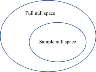
Not null enough: pseudo-null hypotheses in community ecology and comparative psychology

Bayesian data analysis in population ecology: motivations, methods, and benefits.

The multiple-comparison trap and the Raven’s paradox—perils of using null hypothesis testing in environmental assessment

In species co-occurrence studies, when claiming that a species exists, occurs, or is present on an island, ecologists typically mean that the species has established a breeding population on that island instead of just having several vagile individuals.

For a detailed discussion of the differences between neutral models and null models, see Gotelli and McGill ( 2006 ).

In species co-occurrence studies, the null models constructed by different ecologists may be more or less different from each other. Even Connor and Simberloff themselves keep modifying their null models in later publications. Nevertheless, the version I will introduce here, which appears in one of their earliest and also most-cited publications on this subject, helps demonstrate the key features of null-model-based hypothesis testing.

For reviews of the technical issues in the construction of null models, see Gotelli and Graves ( 1996 ) and Sanderson and Pimm ( 2015 ).

Although the term “randomization test” is often used interchangeably with “permutation test,” actually they are different. A randomization test is based on random assignment involved in experimental design; the procedure of random assignment is conducted before empirical data are collected. By contrast, a permutation test is a nonparametric method of statistical hypothesis testing based on data resampling.

Bausman WC (2018) Modeling: neutral, null, and baseline. Philos Sci 85:594–616

Article   Google Scholar  

Bausman W, Halina M (2018) Not null enough: pseudo-null hypotheses in community ecology and comparative psychology. Biol Philos 33:1–20

Chase JM, Leibold MA (2003) Ecological niches: linking classical and contemporary approaches. University of Chicago Press, Chicago

Book   Google Scholar  

Colwell RK, Winkler DW (1984) A null model for null models in biogeography. In: Strong DR Jr, Simberloff D, Abele LG, Thistle AB (eds) Ecological communities: conceptual issues and the evidence. Princeton University Press, Princeton, pp 344–359

Chapter   Google Scholar  

Connor EF, Simberloff D (1979) The assembly of species communities: chance or competition? Ecology 60:1132–1140

Connor EF, Simberloff D (1983) Interspecific competition and species co-occurrence patterns on islands: null models and the evaluation of evidence. Oikos 41:455–465

Connor EF, Simberloff D (1984) Neutral models of species’ co-occurrence patterns. In: Strong DR Jr, Simberloff D, Abele LG, Thistle AB (eds) Ecological communities: conceptual issues and the evidence. Princeton University Press, Princeton, pp 316–331

Connor EF, Collins MD, Simberloff D (2013) The checkered history of checkerboard distributions. Ecology 94:2403–2414

Connor EF, Collins MD, Simberloff D (2015) The checkered history of checkerboard distributions: reply. Ecology 96:3388–3389

Diamond JM (1975) Assembly of species communities. In: Cody ML, Diamond JM (eds) Ecology and evolution of communities. Harvard University Press, Cambridge, pp 342–444

Google Scholar  

Diamond JM, Gilpin ME (1982) Examination of the “null” model of Connor and Simberloff for species co-occurrences on islands. Oecologia 52:64–74

Diamond J, Pimm SL, Sanderson JG (2015) The checkered history of checkerboard distributions: comment. Ecology 96:3386–3388

Fisher RA (1925) Statistical methods for research workers. Oliver and Boyd, Edinburgh

Fisher RA (1926) The arrangement of field experiments. J Minist Agric 33:503–513

Fisher RA (1935) The design of experiments. Oliver and Boyd, Edinburgh

Gilpin ME, Diamond JM (1984) Are species co-occurrences on islands non-random, and are null hypotheses useful in community ecology? In: Strong DR Jr, Simberloff D, Abele LG, Thistle AB (eds) Ecological communities: conceptual issues and the evidence. Princeton University Press, Princeton, pp 297–315

Gotelli NJ, Graves GR (1996) Null models in ecology. Smithsonian Institution Press, Washington

Gotelli NJ, McGill BJ (2006) Null versus neutral models: what’s the difference? Ecography 29:793–800

Harvey PH (1987) On the use of null hypotheses in biogeography. In: Nitechi MH, Hoffman A (eds) Neutral models in biology. Oxford University Press, New York, pp 109–118

Hubbell SP (2001) The unified neutral theory of biodiversity and biogeography. Princeton University Press, Princeton

Hubbell SP (2006) Neutral theory and the evolution of ecological equivalence. Ecology 87:1387–1398

Lewin R (1983) Santa Rosalia was a goat. Science 221:636–639

MacArthur R (1972) Geographical ecology: patterns in the distribution of species. Harper & Row, Publishers, Inc., New York

Rathcke BJ (1984) Patterns of flowering phenologies: testability and causal inference using a random model. In: Strong DR Jr, Simberloff D, Abele LG, Thistle AB (eds) Ecological communities: conceptual issues and the evidence. Princeton University Press, Princeton, pp 383–396

Rosindell J, Hubbell SP, Etienne RS (2011) The unified neutral theory of biodiversity and biogeography at age ten. Trends Ecol Evol 26:340–348

Sanderson JG, Pimm SL (2015) Patterns in nature: the analysis of species co-occurences. The University of Chicago Press, Chicago

Schelling TC (1978) Micromotives and macrobehavior. W. W. Norton & Company, New York

Sloep PB (1986) Null hypotheses in ecology: towards the dissolution of a controversy. Philos Sci 1:307–313

Sober E (1988) Reconstructing the past: parsimony, evolution, and inference. The MIT Press, Cambridge

Sober E (1994) Let’s Razor Ockham’s Razor. In: From a biological point of view. Cambridge University Press, Cambridge, pp 136–157

von Bertalanffy L (1968) General system theory: foundations, development, applications. George Braziller, New York

Download references

Acknowledgements

I wish to acknowledge the great help of Michael Weisberg, Erol Akçay, Jay Odenbaugh, and two anonymous reviewers for suggestions on improving the manuscript. An earlier draft of this article was also presented in the Philosophy of Science Reading Group at the University of Pennsylvania, the Salon of Philosophy of Science and Technology at Tsinghua University in Beijing, and PBDB 13 (Philosophy of Biology at Dolphin Beach) in Moruya, Australia. I want to thank the participants of these meetings, who asked valuable questions that inspired this article.

Author information

Authors and affiliations.

Department of Philosophy, University of Pennsylvania, Claudia Cohen Hall, Room 433, 249 S. 36th Street, Philadelphia, PA, 19104-6304, USA

Mingjun Zhang

You can also search for this author in PubMed   Google Scholar

Corresponding author

Correspondence to Mingjun Zhang .

Additional information

Publisher's note.

Springer Nature remains neutral with regard to jurisdictional claims in published maps and institutional affiliations.

Rights and permissions

Reprints and permissions

About this article

Zhang, M. The use and limitations of null-model-based hypothesis testing. Biol Philos 35 , 31 (2020). https://doi.org/10.1007/s10539-020-09748-0

Download citation

Received : 29 June 2019

Accepted : 13 April 2020

Published : 23 April 2020

DOI : https://doi.org/10.1007/s10539-020-09748-0

Share this article

Anyone you share the following link with will be able to read this content:

Sorry, a shareable link is not currently available for this article.

Provided by the Springer Nature SharedIt content-sharing initiative

• Null hypothesis
• Checkerboard distribution
• Interspecific competition
• Random colonization
• Control of variables
• Find a journal
• Publish with us
• Track your research

Hypothesis Testing in Statistics – Short Notes + PPT

“Truth can be stated in a thousand different ways, yet each one can be true…” Swami Vivekananda

What is ‘Test of Hypothesis’?

Ø   Test of Hypothesis (Hypothesis Testing) is a process of testing of the significance regarding the parameters of the population on the basis of sample drawn from it. Ø   Test of hypothesis is also called as ‘Test of Significance’. Ø   J. Neyman and E.S. Pearson initiated the practice of testing of hypothesis in statistics.

What is the purpose of Hypothesis Testing?

Ø   The main purpose of hypothesis testing is to help the researcher in reaching a conclusion regarding the population by examining a sample taken from that population. Ø   The hypothesis testing does not provide proof for the hypothesis. Ø   The test only indicates whether the hypothesis is supported or not supported by the available data.

What is Hypothesis?

Ø   Hypothesis is a statement about one or more populations.

Ø   It is a statement about the parameters of the population about which the statement is made.

Ø   Example:

$   A doctor hypothesized: “The drug ‘X’ is ineffective in 99% of cases of which it is used”.

$   “The average pass percentage of central university degree programme is 98”.

Ø   Through the hypothesis testing the researcher or investigator can determine whether or not such statements are compatible with the available data.

Types of Hypothesis

Ø   There are TWO types of hypothesis.

                        (A).   Research Hypothesis

                        (B).   Statistical Hypothesis

(A). Research Hypothesis

Ø   Research Hypothesis is “a tentative solution for the problem being investigated”.

Ø   It is the supposition (guess) that motivates the research.

Ø   In research, the researcher determines whether or not their supposition can be supported through scientific investigation.

Ø   The research hypothesis directly leads to statistical hypothesis.

(B). Statistical Hypothesis

Details of the Statistical hypothesis are discussed in the “Steps or Components in Testing of Statistical Hypothesis”.

Steps / Components in Testing of Statistical Hypothesis:

Ø   The statistical hypothesis testing consists of following Steps / Components

(1).      Data (variable)

(2).      Statistical Hypothesis

(3).      Test Statistic

(4).      Decision Rule

(5).      Significance Level

(6).      Statistical Decision

(7).      p – Value

(1). Data (variable)

Ø   Data is the information collected from the population.

Ø   It may be the observation of a natural phenomenon, Result of an experiment, Data from a survey or a secondary data.

Ø   The nature of data determines the type of statistical test to be selected.

Ø   All the features of the data such as continuous, discontinuous, quantitative or qualitative etc. matters in the process of hypothesis testing.

(2). Statistical Hypothesis

Ø   Statistical hypothesis is a statement about the population which we want to verify on the basis of information available from the sample.

Ø   A statistical hypothesis is stated in such a way that they may be evaluated by appropriate statistical techniques.

Ø   There are TWO types of statistical hypothesizes:

(a).  Null hypothesis

(b).  Alternative hypothesis

(a). Null Hypothesis

Ø   The Null hypothesis is the hypothesis to be tested by test statistic.

Ø  Null hypothesis is denoted as H 0 .

Ø   Usually the null hypothesis stated as the ‘Hypothesis of No Difference’.

Ø   The statement is created complementary to the conclusion that the researcher is seeking to reach through his research.

Ø   Usually stated in the negative terms of the original research hypothesis.

Ø   Example: The drug ‘X’ DO NOT induces apoptosis in cancerous cells.

Ø   In the statistical testing process, the null hypothesis is either:

$   Rejected

$   Not rejected (Fail to be rejected / accepted)

Ø   If the null hypothesis is not rejected, we say that the data on which the test is based do not provide sufficient evidence to cause the rejection of null hypothesis.

Ø   If the null hypothesis is rejected in the testing process, we say that the data at hand are not compatible with the null hypothesis but are supportive for some other hypothesis (commonly called as alternative hypothesis).

(b). Alternative Hypothesis

Ø   Alternate hypothesis is created in a negative meaning of the null hypothesis.

Ø   It is denoted as H 1 or H A .

Ø   Usually the alternative hypothesis and research hypothesis are the same.

Ø   Example: The drug ‘X’ induces apoptosis in cancerous cells.

How to state the statistical hypothesis?

Ø   The null hypothesis should contain an equality sign (=, ≤ or ≥).

Ø   Example: The population mean (μ) is not 100.

$   H0:       μ = 100

$   H1:       μ ≠ 100

Ø   Example: The population means is greater than 100.

$   H0:       μ ≤ 100

$   H1:       μ > 100

Ø   Example: The population mean is less than 100.

$   H0:       μ ≥ 100

$   H1:       μ < 100

Things to remember when constructing the Null Hypothesis:

$   What you expected to conclude with the study should be placed in the alternative hypothesis.

$   The null hypothesis should contain a statement of equality (=, ≤, ≥).

$   The null hypothesis is the hypothesis to be tested.

$   The null hypothesis and alternative hypothesis should be complementary.

(3). Test Statistic

Ø   Test statistic is the statistic computed from the data sample.

Ø   There are many possible values that the test statistic can adopt.

Ø   Test value of the statistic depends on the nature of the sample.

Ø   The test statistic is the decision maker in hypothesis testing.

Ø   Decision is to reject or not reject the null hypothesis.

Ø   General formula for test statistic: (applicable to most of the test statistic but not to all)

x̄            : mean

μ0         : hypothesized value of population mean

σ/√n     : Standard error

(4). Decision Rule

Ø   All the possible values that the test statistic can assume are points on the horizontal axis of a graph of the distribution of the test statistic.

Ø   The values are divided into two groups:

1.      Values of the rejection region

2.      Values of the non-rejection region

Ø   The decision rule tell us to reject the null hypothesis if the values of the test statistic that we compute from our sample is one of the values in the rejection region and not to reject the null hypothesis if the computed values of the test statistic is on the values in the non-rejection region.

(5) Significance Level

Ø   Level of significance is the probability of rejecting a true null hypothesis in the statistical testing procedure.

Ø   The level of significance is a probability value and it is denoted as ‘α’.

Ø   The significance level decide the decision value to go the rejection region or to the non-rejection region.

Ø  Due to the ‘Level of significance’ the test statistic is often called as ‘Significance Test’.

Ø   If we reject a true null hypothesis we are committed an error.

Ø   Thus, you have to ensure that the probability of rejecting a true null hypothesis is very small.

Ø   Thus, we select a small value of α to ensure the probability of rejecting a true null hypothesis is very less.

Ø   The frequently used α values are 0.01 (99%), 0.05 (95%).

Ø   Explanation : if we select 0.01 (99%) as the significance level, it means that we are 99% confident in our decision but still there is 1% change for our decision being false.

(6). Statistical Decision

Ø   It is the decision of rejecting or not rejecting the null hypothesis.

Ø   We reject the null hypothesis if the computed value of the test statistic is fall in the rejection region.

Ø   We will NOT reject the null hypothesis if the computed value falls in the non-rejection region.

Ø   Conclusion:

Ø   If we reject H 0 , we conclude that H A is true.

Ø   If we fail to reject H 0 , we conclude that the H 0 may be true.

Ø   When a null hypothesis is not rejected one should not say that the null hypothesis accepted but we say that null hypothesis is not rejected.

Ø   We usually avoid the usage ‘accept’, because we may have committed a type II error.

Learn more: Statistical Errors (Type I and Type II Errors)

(7). p-Value

Ø   p-value is the smallest value of α for which we can reject a null hypothesis.

Ø   A p-value is the probability that the computed value for a test statistic is at least as extreme as specified value of the test statistic when the null hypothesis is true.

Daniel, W.W., 1999. Biostatistics: A foundation for analysis in the health sciences 9th edition. John Wiley & Sons inc.: USA.

Khan, I.A. and Khanum, A., 2012, Fundamentals of Biostatistics, 3rd edition (revised), Ukaaz Publications, Hyderabad, India.

Kothari, C.R., 2004. Research methodology: Methods and techniques. New Age International, India.

<<< Back to Statistics Note Papte

Do you have any Queries? Please leave me a COMMENT in the Comments Section below. I will be Happy to Read your Comments and Reply.

Download the PPT of this Topic

You might also like…

@. Introduction to Biostatistics

@. Data Collection Methods in Statistics

@. Difference between Type I and Type II Errors

@. Biostatistics PPTs.

More Lecture Notes from Easy Biology Class…

Botany Zoology Biochemistry Genetics Molecular Biology Biotechnology Endocrinology Physiology Microbiology Immunology Embryology Ecology Evolution Biophysics Research Methodology Biostatistics Chemistry for Biologists Physics for Biologists

Browse more in Easy Biology Class…

Lecture Notes Biology PPTs Video Tutorials Biology MCQ Question Bank Difference between Practical Aids Mock Tests (Online) Biology Exams

Related posts:

• Principles of Experimental Designs in Statistics – Replication, Randomization & Local Control
• Types of Experimental Designs in Statistics (RBD, CRD, LSD, Factorial Designs)
• Difference between Primary and Secondary Data
• MCQ on Hypothesis Testing in Statistics
• What is Data in Statistics?

Leave a Reply Cancel reply

Your email address will not be published. Required fields are marked *

Privacy Overview

Statistics Made Easy

5 Tips for Interpreting P-Values Correctly in Hypothesis Testing

Hypothesis testing is a critical part of statistical analysis and is often the endpoint where conclusions are drawn about larger populations based on a sample or experimental dataset. Central to this process is the p-value. Broadly, the p-value quantifies the strength of evidence against the null hypothesis. Given the importance of the p-value, it is essential to ensure its interpretation is correct. Here are five essential tips for ensuring the p-value from a hypothesis test is understood correctly. 

1. Know What the P-value Represents

First, it is essential to understand what a p-value is. In hypothesis testing, the p-value is defined as the probability of observing your data, or data more extreme, if the null hypothesis is true. As a reminder, the null hypothesis states no difference between your data and the expected population. 

For example, in a hypothesis test to see if changing a company’s logo drives more traffic to the website, a null hypothesis would state that the new traffic numbers are equal to the old traffic numbers. In this context, the p-value would be the probability that the data you observed, or data more extreme, would occur if this null hypothesis were true. 

Therefore, a smaller p-value indicates that what you observed is unlikely to have occurred if the null were true, offering evidence to reject the null hypothesis. Typically, a cut-off value of 0.05 is used where any p-value below this is considered significant evidence against the null. 

2. Understand the Directionality of Your Hypothesis

Based on the research question under exploration, there are two types of hypotheses: one-sided and two-sided. A one-sided test specifies a particular direction of effect, such as traffic to a website increasing after a design change. On the other hand, a two-sided test allows the change to be in either direction and is effective when the researcher wants to see any effect of the change. 

Either way, determining the statistical significance of a p-value is the same: if the p-value is below a threshold value, it is statistically significant. However, when calculating the p-value, it is important to ensure the correct sided calculations have been completed. 

Additionally, the interpretation of the meaning of a p-value will differ based on the directionality of the hypothesis. If a one-sided test is significant, the researchers can use the p-value to support a statistically significant increase or decrease based on the direction of the test. If a two-sided test is significant, the p-value can only be used to say that the two groups are different, but not that one is necessarily greater. 

3. Avoid Threshold Thinking

A common pitfall in interpreting p-values is falling into the threshold thinking trap. The most commonly used cut-off value for whether a calculated p-value is statistically significant is 0.05. Typically, a p-value of less than 0.05 is considered statistically significant evidence against the null hypothesis. 

However, this is just an arbitrary value. Rigid adherence to this or any other predefined cut-off value can obscure business-relevant effect sizes. For example, a hypothesis test looking at changes in traffic after a website design may find that an increase of 10,000 views is not statistically significant with a p-value of 0.055 since that value is above 0.05. However, the actual increase of 10,000 may be important to the growth of the business. 

Therefore, a p-value can be practically significant while not being statistically significant. Both types of significance and the broader context of the hypothesis test should be considered when making a final interpretation. 

4. Consider the Power of Your Study

Similarly, some study conditions can result in a non-significant p-value even if practical significance exists. Statistical power is the ability of a study to detect an effect when it truly exists. In other words, it is the probability that the null hypothesis will be rejected when it is false. 

Power is impacted by a lot of factors. These include sample size, the effect size you are looking for, and variability within the data. In the example of website traffic after a design change, if the number of visits overall is too small, there may not be enough views to have enough power to detect a difference. 

Simple ways to increase the power of a hypothesis test and increase the chances of detecting an effect are increasing the sample size, looking for a smaller effect size, changing the experiment design to control for variables that can increase variability, or adjusting the type of statistical test being run.

5. Be Aware of Multiple Comparisons

Whenever multiple p-values are calculated in a single study due to multiple comparisons, there is an increased risk of false positives. This is because each individual comparison introduces random fluctuations, and each additional comparison compounds these fluctuations. 

For example, in a hypothesis test looking at traffic before and after a website redesign, the team may be interested in making more than one comparison. This can include total visits, page views, and average time spent on the website. Since multiple comparisons are being made, there must be a correction made when interpreting the p-value. 

The Bonferroni correction is one of the most commonly used methods to account for this increased probability of false positives. In this method, the significance cut-off value, typically 0.05, is divided by the number of comparisons made. The result is used as the new significance cut-off value.  Applying this correction mitigates the risk of false positives and improves the reliability of findings from a hypothesis test. 

In conclusion, interpreting p-values requires a nuanced understanding of many statistical concepts and careful consideration of the hypothesis test’s context. By following these five tips, the interpretation of the p-value from a hypothesis test can be more accurate and reliable, leading to better data-driven decision-making.

Featured Posts

Leave a Reply Cancel reply

Your email address will not be published. Required fields are marked *

Join the Statology Community

Sign up to receive Statology's exclusive study resource: 100 practice problems with step-by-step solutions. Plus, get our latest insights, tutorials, and data analysis tips straight to your inbox!

By subscribing you accept Statology's Privacy Policy.

share this!

May 28, 2024

This article has been reviewed according to Science X's editorial process and policies . Editors have highlighted the following attributes while ensuring the content's credibility:

fact-checked

trusted source

Why do dyeing poison frogs tap dance?

by Ananya Sen, University of Illinois at Urbana-Champaign

The toe tapping behavior of various amphibians has long attracted attention from researchers and pet owners. Despite being widely documented, the underlying functional role is poorly understood. In a new paper, researchers demonstrate that dyeing poison frogs modulate their taps based on specific stimuli. The research is published in the journal Ethology .

Dyeing poison frogs, Dendrobates tinctorius, have been shown to tap their posterior toes in response to a range of prey sizes, from small fruit flies to large crickets. In the present study, the researchers hypothesized that if the tapping has a role in feeding, the frogs would adjust their behavior in response to different environmental cues.

To test their hypothesis, the researchers recorded the frogs under varying conditions.

"I used the slow-motion camera on my iPhone to take minute-long videos of the frogs tapping. Afterwards, I went back to each video and counted the number of taps on each foot and how long they were visible since they were often hidden behind a leaf or the frog itself. I used those two numbers to get a 'taps per minute' on each foot and added them up," said Thomas Parrish, a former undergraduate student in the Fischer lab (GNDP), and the first author on the paper.

The researchers first tested whether the frogs tapped their toes more when they were feeding. To do so, the researchers fed the terrariums with half a teaspoon of fruit flies and recorded their hunting.

"We already knew the answer to this, but it was great to see that the tapping increased in the presence of the prey," said Eva Fischer, an assistant professor of integrative biology. "We wanted to ask 'Why?' and we wondered whether it had a function in prey capture or it was just a excitatory response like how dogs wag their tails because they are excited."

The researchers then used different surfaces to see whether the tapping behavior changed when the frogs could see the prey but not feed on it. They placed the fruit flies in small, clear Petri dishes in the frogs' home and measured the rate of toe tapping. They found that the frogs had an average of 50 taps/minute when they couldn't access the flies compared to 166 taps/minute when they fed on free-moving flies.

"The idea was that if they're excited, we might see something different based on whether they can catch the flies," Fisher said. "These results suggested that since they kept trying to eat in both cases, the tapping was not just out of excitement."

The researchers wondered, then, whether the toe taps were a form of vibrational signaling where the frogs used it as a way to startle or distract the prey before they fed. They used four different surfaces to test this question: soil, leaf surfaces, gel, and glass.

"Soil and leaves are natural substances, but soil is not very responsive while leaves are. On the other hand, gels are responsive and glass is not, but they are both unnatural surfaces to frogs," Fischer said.

They found that while the tap rate differed depending on the surface, with leaves being the highest at 255 taps/minute and glass the lowest at 64 taps/minute, there was no difference in the total number of feeding attempts or success.

"Although we saw that the frogs ate in every context, it was exciting to see that they changed their behavior based on what they're standing on," Fischer said. "We were surprised, however, that we didn't see a difference in how successful they were at eating. It's possible that the experiment is like sending them to a buffet instead of what happens in the forest where the tapping may help in stirring the prey ."

The researchers are now hoping to understand what other stimuli might trigger this behavior. "Although we've conclusively shown that it is important in feeding, it could also be important in other contexts. For example, we have seen that the frogs tap more when there are other frogs nearby, so there may be a social aspect to it," Fischer said.

They are also interested in studying the underlying biomechanical aspects of the muscles. "It would be cool to look at the anatomy and see how the muscles work," Fischer said. "Ultimately, we could ask whether all frogs can tap their toes if they have the right muscles or whether there's something special about the anatomy of poison frogs ."

Provided by University of Illinois at Urbana-Champaign

Explore further

Feedback to editors

How worms shaped Earth's biodiversity explosion

2 hours ago

Meet Neo Px: the super plant that attacks air pollution

A Chinese spacecraft lands on the moon's far side to collect rocks in growing space rivalry with US

Saturday Citations: The sound of music, sneaky birds, better training for LLMs. Plus: Diversity improves research

23 hours ago

Study investigates a massive 'spider' pulsar

Jun 1, 2024

Greener, more effective termite control: Natural compound attracts wood eaters

Shear genius: Researchers find way to scale up wonder material, which could do wonders for the Earth

New vestiges of the first life on Earth discovered in Saudi Arabia

May 31, 2024

Mussels downstream of wastewater treatment plant contain radium, study reports

A new way to see viruses in action: Super-resolution microscopy provides a nano-scale look

Relevant physicsforums posts, a dna animation.

May 29, 2024

Probability, genetic disorder related

Looking for today's dna knowledge.

May 27, 2024

Covid Vaccines Reducing Infections

Human sperm, egg cells mass-generated using ips, and now, here comes covid-19 version ba.2, ba.4, ba.5,....

May 25, 2024

More from Biology and Medical

Related Stories

'Time to eat': Videos show that toe-tapping by frogs may be a strategy to draw out prey

Feb 6, 2024

Young frogs may camouflage selves as animal poo: study

Oct 12, 2023

Australian mosquito species found to target frogs' noses

Nov 28, 2023

Wanted: Photos of frogs being fed on by flies (for frog conservation)

Jun 21, 2022

130 poisonous frogs seized at Bogota airport

Jan 30, 2024

Invasive, carnivorous frogs are now breeding in Georgia, biologists say

Jan 5, 2024

Recommended for you

This tiny fern has the largest genome of any organism on Earth

Scientists map biodiversity changes in the world's forests

Jumping spider study finds offspring care extends lifespan of mothers

The missing puzzle piece: A striking new snake species from the Arabian Peninsula

May 30, 2024

Let us know if there is a problem with our content

Use this form if you have come across a typo, inaccuracy or would like to send an edit request for the content on this page. For general inquiries, please use our contact form . For general feedback, use the public comments section below (please adhere to guidelines ).

Please select the most appropriate category to facilitate processing of your request

Thank you for taking time to provide your feedback to the editors.

Your feedback is important to us. However, we do not guarantee individual replies due to the high volume of messages.

E-mail the story

Your email address is used only to let the recipient know who sent the email. Neither your address nor the recipient's address will be used for any other purpose. The information you enter will appear in your e-mail message and is not retained by Phys.org in any form.

Newsletter sign up

Get weekly and/or daily updates delivered to your inbox. You can unsubscribe at any time and we'll never share your details to third parties.

More information Privacy policy

Donate and enjoy an ad-free experience

We keep our content available to everyone. Consider supporting Science X's mission by getting a premium account.

E-mail newsletter

Gene variants foretell the biology of future breast cancers

A Stanford Medicine study of thousands of breast cancers has found that the gene sequences we inherit at conception are powerful predictors of the breast cancer type we might develop decades later and how deadly it might be.

The study challenges the dogma that most cancers arise as the result of random mutations that accumulate during our lifetimes. Instead, it points to the active involvement of gene sequences we inherit from our parents -- what's known as your germline genome -- in determining whether cells bearing potential cancer-causing mutations are recognized and eliminated by the immune system or skitter under the radar to become nascent cancers.

"Apart from a few highly penetrant genes that confer significant cancer risk, the role of heredity factors remains poorly understood, and most malignancies are assumed to result from random errors during cell division or bad luck," said Christina Curtis, PhD, the RZ Cao Professor of Medicine and a professor of genetics and of biomedical data science. "This would imply that tumor initiation is random, but that is not what we observe. Rather, we find that the path to tumor development is constrained by hereditary factors and immunity. This new result unearths a new class of biomarkers to forecast tumor progression and an entirely new way of understanding breast cancer origins."

Curtis is the senior author of the study, which will be published May 31 in Science . Postdoctoral scholar Kathleen Houlahan, PhD, is the lead author of the research.

"Back in 2015, we had posited that some tumors are 'born to be bad' -- meaning that their malignant and even metastatic potential is determined early in the disease course," Curtis said. "We and others have since corroborated this finding across multiple tumors, but these findings cast a whole new light on just how early this happens."

A new take on cancer's origin

The study, which gives a nuanced and powerful new understanding of the interplay between newly arisen cancer cells and the immune system, is likely to help researchers and clinicians better predict and combat breast tumors.

Currently, only a few high-profile cancer-associated mutations in genes are regularly used to predict cancers. Those include BRCA1 and BRCA2, which occur in about one of every 500 women and confer an increased risk of breast or ovarian cancer, and rarer mutations in a gene called TP53 that causes a disease called Li Fraumeni syndrome, which predisposes to childhood and adult-onset tumors.

The findings indicate there are tens or hundreds of additional gene variants -- identifiable in healthy people -- pulling the strings that determine why some people remain cancer-free throughout their lives.

"Our findings not only explain which subtype of breast cancer an individual is likely to develop," Houlahan said, "but they also hint at how aggressive and prone to metastasizing that subtype will be. Beyond that, we anticipate that these inherited variants may influence a person's risk of developing breast cancer."

The genes we inherit from our parents are known as our germline genome. They're mirrors of our parents' genetic makeup, and they can vary among people in small ways that give some of us blue eyes, brown hair or type O blood. Some inherited genes include mutations that confer increased cancer risk from the get-go, such as BRCA1, BRCA2 and TP53. But identifying other germline mutations strongly associated with future cancers has proven difficult.

In contrast, most cancer-associated genes are part of what's known as our somatic genome. As we live our lives, our cells divide and die in the tens of millions. Each time the DNA in a cell is copied, mistakes happen and mutations can accumulate. DNA in tumors is often compared with the germline genomes in blood or normal tissues in an individual to pinpoint which changes likely led to the cell's cancerous transformation.

Classifying breast cancers

In 2012, Curtis began a deep dive -- assisted by machine learning -- into the types of somatic mutations that occur in thousands of breast cancers. She was eventually able to categorize the disease into 11 subtypes with varying prognoses and risk of recurrence, finding that four of the 11 groups were significantly more likely to recur even 10 or 20 years after diagnosis -- critical information for clinicians making treatment decisions and discussing long-term prognoses with their patients.

Prior studies had shown that people with inherited BRCA1 or BRCA2 mutations tend to develop a subtype of breast cancer known as triple negative breast cancer. This correlation implies some behind-the-scenes shenanigans by the germline genome that affects what subtype of breast cancer someone might develop.

"We wanted to understand how inherited DNA might sculpt how a tumor evolves," Houlahan said. To do so, they took a close look at the immune system.

It's a quirk of biology that even healthy cells routinely decorate their outer membranes with small chunks of the proteins they have bobbing in their cytoplasm -- an outward display that reflects their inner style.

The foundations for this display are what's known as HLA proteins, and they are highly variable among individuals. Like fashion police, immune cells called T cells prowl the body looking for any suspicious or overly flashy bling (called epitopes) that might signal something is amiss inside the cell. A cell infected with a virus will display bits of viral proteins; a sick or cancerous cell will adorn itself with abnormal proteins. These faux pas trigger the T cells to destroy the offenders.

Houlahan and Curtis decided to focus on oncogenes, normal genes that, when mutated, can free a cell from regulatory pathways meant to keep it on the straight and narrow. Often, these mutations take the form of multiple copies of the normal gene, arranged nose to tail along the DNA -- the result of a kind of genomic stutter called amplification. Amplifications in specific oncogenes drive different cancer pathways and were used to differentiate one breast cancer subtype from another in Curtis' original studies.

The importance of bling

The researchers wondered whether highly recognizable epitopes would be more likely to attract T cells' attention than other, more modest displays (think golf-ball-sized, dangly turquoise earrings versus a simple silver stud). If so, a cell that had inherited a flashy version of an oncogene might be less able to pull off its amplification without alerting the immune system than a cell with a more modest version of the same gene. (One pair of overly gaudy turquoise earrings can be excused; five pairs might cause a patrolling fashionista T cell to switch from tutting to terminating.)

The researchers studied nearly 6,000 breast tumors spanning various stages of disease to learn whether the subtype of each tumor correlated with the patients' germline oncogene sequences. They found that people who had inherited an oncogene with a high germline epitope burden (read: lots of bling) -- and an HLA type that can display that epitope prominently -- were significantly less likely to develop breast cancer subtypes in which that oncogene is amplified.

There was a surprise, though. The researchers found that cancers with a large germline epitope burden that manage to escape the roving immune cells early in their development tended to be more aggressive and have a poorer prognosis than their more subdued peers.

"At the early, pre-invasive stage, a high germline epitope burden is protective against cancer," Houlahan said. "But once it's been forced to wrestle with the immune system and come up with mechanisms to overcome it, tumors with high germline epitope burden are more aggressive and prone to metastasis. The pattern flips during tumor progression."

"Basically, there is a tug of war between tumor and immune cells," Curtis said. "In the preinvasive setting, the nascent tumor may initially be more susceptible to immune surveillance and destruction. Indeed, many tumors are likely eliminated in this manner and go unnoticed. However, the immune system does not always win. Some tumor cells may not be eliminated and those that persist develop ways to evade immune recognition and destruction. Our findings shed light on this opaque process and may inform the optimal timing of therapeutic intervention, as well as how to make an immunologically cold tumor become hot, rendering it more sensitive to therapy."

The researchers envision a future when the germline genome is used to further stratify the 11 breast cancer subtypes identified by Curtis to guide treatment decisions and improve prognoses and monitoring for recurrence. The study's findings may also give additional clues in the hunt for personalized cancer immunotherapies and may enable clinicians to one day predict a healthy person's risk of cancer from a simple blood sample.

"We started with a bold hypothesis," Curtis said. "The field had not thought about tumor origins and evolution in this way. We're examining other cancers through this new lens of heredity and acquired factors and tumor-immune co-evolution."

The study was funded by the National Institutes of Health (grants DP1-CA238296 and U54CA261719), the Canadian Institutes of Health Research and the Chan Zuckerberg Biohub.

• Breast Cancer
• Brain Tumor
• Lung Cancer
• Colon Cancer
• Diseases and Conditions
• Ovarian Cancer
• Breast cancer
• Monoclonal antibody therapy
• Mammography
• Breast implant
• Colorectal cancer
• Breast reconstruction

Story Source:

Materials provided by Stanford Medicine . Original written by Krista Conger. Note: Content may be edited for style and length.

Journal Reference :

• Kathleen E. Houlahan, Aziz Khan, Noah F. Greenwald, Cristina Sotomayor Vivas, Robert B. West, Michael Angelo, Christina Curtis. Germline-mediated immunoediting sculpts breast cancer subtypes and metastatic proclivity . Science , 2024; 384 (6699) DOI: 10.1126/science.adh8697

Cite This Page :

Explore More

• How Statin Therapy May Prevent Cancer
• Origins of 'Welsh Dragons' Exposed
• Resting Brain: Neurons Rehearse for Future
• Observing Single Molecules
• A Greener, More Effective Way to Kill Termites
• One Bright Spot Among Melting Glaciers
• Martian Meteorites Inform Red Planet's Structure
• Volcanic Events On Jupiter's Moon Io: High Res
• What Negative Adjectives Mean to Your Brain
• 'Living Bioelectronics' Can Sense and Heal Skin

Trending Topics

Strange & offbeat.