data representation categories

• school Campus Bookshelves
• menu_book Bookshelves
• perm_media Learning Objects
• login Login
• how_to_reg Request Instructor Account
• hub Instructor Commons
• Download Page (PDF)
• Download Full Book (PDF)
• Periodic Table
• Physics Constants
• Scientific Calculator
• Reference & Cite
• Tools expand_more
• Readability

selected template will load here

This action is not available.

2.1: Types of Data Representation

• Last updated
• Save as PDF
• Page ID 5696

Two common types of graphic displays are bar charts and histograms. Both bar charts and histograms use vertical or horizontal bars to represent the number of data points in each category or interval. The main difference graphically is that in a  bar chart  there are spaces between the bars and in a  histogram  there are not spaces between the bars. Why does this subtle difference exist and what does it imply about graphic displays in general?

Displaying Data

It is often easier for people to interpret relative sizes of data when that data is displayed graphically. Note that a  categorical variable  is a variable that can take on one of a limited number of values and a  quantitative variable  is a variable that takes on numerical values that represent a measurable quantity. Examples of categorical variables are tv stations, the state someone lives in, and eye color while examples of quantitative variables are the height of students or the population of a city. There are a few common ways of displaying data graphically that you should be familiar with. 

A  pie chart  shows the relative proportions of data in different categories.  Pie charts  are excellent ways of displaying categorical data with easily separable groups. The following pie chart shows six categories labeled A−F.  The size of each pie slice is determined by the central angle. Since there are 360 o  in a circle, the size of the central angle θ A  of category A can be found by:

CK-12 Foundation -  https://www.flickr.com/photos/slgc/16173880801  - CCSA

A  bar chart  displays frequencies of categories of data. The bar chart below has 5 categories, and shows the TV channel preferences for 53 adults. The horizontal axis could have also been labeled News, Sports, Local News, Comedy, Action Movies. The reason why the bars are separated by spaces is to emphasize the fact that they are categories and not continuous numbers. For example, just because you split your time between channel 8 and channel 44 does not mean on average you watch channel 26. Categories can be numbers so you need to be very careful.

CK-12 Foundation -  https://www.flickr.com/photos/slgc/16173880801  - CCSA

A  histogram  displays frequencies of quantitative data that has been sorted into intervals. The following is a histogram that shows the heights of a class of 53 students. Notice the largest category is 56-60 inches with 18 people.

A  boxplot  (also known as a  box and whiskers plot ) is another way to display quantitative data. It displays the five 5 number summary (minimum, Q1,  median , Q3, maximum). The box can either be vertically or horizontally displayed depending on the labeling of the axis. The box does not need to be perfectly symmetrical because it represents data that might not be perfectly symmetrical.

Earlier, you were asked about the difference between histograms and bar charts. The reason for the space in bar charts but no space in histograms is bar charts graph categorical variables while histograms graph quantitative variables. It would be extremely improper to forget the space with bar charts because you would run the risk of implying a spectrum from one side of the chart to the other. Note that in the bar chart where TV stations where shown, the station numbers were not listed horizontally in order by size. This was to emphasize the fact that the stations were categories.

Create a boxplot of the following numbers in your calculator.

8.5, 10.9, 9.1, 7.5, 7.2, 6, 2.3, 5.5

Enter the data into L1 by going into the Stat menu.

CK-12 Foundation - CCSA

Then turn the statplot on and choose boxplot.

Use Zoomstat to automatically center the window on the boxplot.

Create a pie chart to represent the preferences of 43 hungry students.

• Other – 5
• Burritos – 7
• Burgers – 9
• Pizza – 22

Create a bar chart representing the preference for sports of a group of 23 people.

• Football – 12
• Baseball – 10
• Basketball – 8
• Hockey – 3

Create a histogram for the income distribution of 200 million people.

• Below $50,000 is 100 million people
• Between $50,000 and $100,000 is 50 million people
• Between $100,000 and $150,000 is 40 million people
• Above $150,000 is 10 million people

1. What types of graphs show categorical data?

2. What types of graphs show quantitative data?

A math class of 30 students had the following grades:

3. Create a bar chart for this data.

4. Create a pie chart for this data.

5. Which graph do you think makes a better visual representation of the data?

A set of 20 exam scores is 67, 94, 88, 76, 85, 93, 55, 87, 80, 81, 80, 61, 90, 84, 75, 93, 75, 68, 100, 98

6. Create a histogram for this data. Use your best judgment to decide what the intervals should be.

7. Find the  five number summary  for this data.

8. Use the  five number summary  to create a boxplot for this data.

9. Describe the data shown in the boxplot below.

10. Describe the data shown in the histogram below.

A math class of 30 students has the following eye colors:

11. Create a bar chart for this data.

12. Create a pie chart for this data.

13. Which graph do you think makes a better visual representation of the data?

14. Suppose you have data that shows the breakdown of registered republicans by state. What types of graphs could you use to display this data?

15. From which types of graphs could you obtain information about the spread of the data? Note that spread is a measure of how spread out all of the data is.

Review (Answers)

To see the Review answers, open this  PDF file  and look for section 15.4. 

Additional Resources

PLIX: Play, Learn, Interact, eXplore - Baby Due Date Histogram

Practice: Types of Data Representation

Real World: Prepare for Impact

• Comprehensive Learning Paths
• 150+ Hours of Videos
• Complete Access to Jupyter notebooks, Datasets, References.

Types of Data in Statistics – A Comprehensive Guide

• September 15, 2023

Statistics is a domain that revolves around the collection, analysis, interpretation, presentation, and organization of data. To appropriately utilize statistical methods and produce meaningful results, understanding the types of data is crucial.

In this Blog post we will learn

• Qualitative Data (Categorical Data) 1.1. Nominal Data: 1.2. Ordinal Data:
• Quantitative Data (Numerical Data) 2.1. Discrete Data: 2.2. Continuous Data:
• Time-Series Data:

Let’s explore the different types of data in statistics, supplemented with examples and visualization methods using Python.

1. Qualitative Data (Categorical Data)

We often term qualitative data as categorical data, and you can divide it into categories, but you cannot measure or quantify it.

1.1. Nominal Data:

Nominal data represents categories or labels without any inherent order, ranking, or numerical significance as a type of categorical data. In other words, nominal data classifies items into distinct groups or classes based on some qualitative characteristic, but the categories have no natural or meaningful order associated with them.

Key Characteristics

No Quantitative Meaning: Unlike ordinal, interval, or ratio data, nominal data does not imply any quantitative or numerical meaning. The categories are purely qualitative and serve as labels for grouping.

Arbitrary Assignment: The assignment of items to categories in nominal data is often arbitrary and based on some subjective or contextual criteria. For example, assigning items to categories like “red,” “blue,” or “green” for colors is arbitrary.

No Mathematical Operations: Arithmetic operations like addition, subtraction, or multiplication are not meaningful with nominal data because there is no numerical significance to the categories.

Examples of nominal data include:

• Gender categories (e.g., “male,” “female,” “other”).
• Marital status (e.g., “single,” “married,” “divorced,” “widowed”).
• Types of animals (e.g., “cat,” “dog,” “horse,” “bird”).
• Ethnicity or race (e.g., “Caucasian,” “African American,” “Asian,” “Hispanic”).

1.2. Ordinal Data:

Ordinal data is a type of categorical data that represents values with a meaningful order or ranking but does not have a consistent or evenly spaced numerical difference between the values. In other words, ordinal data has categories that can be ordered or ranked, but the intervals between the categories are not uniform or measurable.

Non-Numeric Labels: The categories in ordinal data are typically represented by non-numeric labels or symbols, such as “low,” “medium,” and “high” for levels of satisfaction or “small,” “medium,” and “large” for T-shirt sizes.

No Fixed Intervals: Unlike interval or ratio data, where the intervals between values have a consistent meaning and can be measured, ordinal data does not have fixed or uniform intervals. In other words, you cannot say that the difference between “low” and “medium” is the same as the difference between “medium” and “high.”

Limited Arithmetic Operations: Arithmetic operations like addition and subtraction are not meaningful with ordinal data because the intervals between categories are not quantifiable. However, some basic operations like counting frequencies, calculating medians, or finding modes can still be performed.

Examples of ordinal data include:

• Educational attainment levels (e.g., “high school,” “bachelor’s degree,” “master’s degree”).
• Customer satisfaction ratings (e.g., “very dissatisfied,” “somewhat dissatisfied,” “neutral,” “satisfied,” “very satisfied”).
• Likert scale responses (e.g., “strongly disagree,” “disagree,” “neutral,” “agree,” “strongly agree”).

2. Quantitative Data (Numerical Data)

Quantitative data represents quantities and can be measured.

2.1. Discrete Data:

Discrete data refers to a type of data that consists of distinct, separate values or categories. These values are typically counted and are often whole numbers, although they don’t have to be limited to integers. Discrete data can only take on specific, finite values within a defined range.

Key characteristics of discrete data include:

a. Countable Values : Discrete data represents individual, separate items or categories that can be counted or enumerated. For example, the number of students in a classroom, the number of cars in a parking lot, or the number of pets in a household are all discrete data.

b. Distinct Categories : Each value in discrete data represents a distinct category or class. These categories are often non-overlapping, meaning that an item can belong to one category only, with no intermediate values.

c. Gaps between Values : There are gaps or spaces between the values in discrete data. For example, if you are counting the number of people in a household, you can have values like 1, 2, 3, and so on, but you can’t have values like 1.5 or 2.75.

d. Often Represented Graphically with Bar Charts : Discrete data is commonly visualized using bar charts or histograms, where each category is represented by a separate bar, and the height of the bar corresponds to the frequency or count of that category.

* Examples of discrete data include:

The number of children in a family. The number of defects in a batch of products. The number of goals scored by a soccer team in a season. The number of days in a week (Monday, Tuesday, etc.). The types of cars in a parking lot (sedan, SUV, truck).

2.2. Continuous Data:

Continuous data, also known as continuous variables or quantitative data, is a type of data that can take on an infinite number of values within a given range. It represents measurements that can be expressed with a high level of precision and are typically numeric in nature. Unlike discrete data, which consists of distinct, separate values, continuous data can have values at any point along a continuous scale.

Precision: Continuous data is often associated with high precision, meaning that measurements can be made with great detail. For example, temperature, height, and weight can be measured to multiple decimal places.

No Gaps or Discontinuities: There are no gaps, spaces, or jumps between values in continuous data. You can have values that are very close to each other without any distinct categories or separations.

Graphical Representation: Continuous data is commonly visualized using line charts or scatter plots, where data points are connected with lines to show the continuous nature of the data.

Examples of continuous data include:

• Temperature readings, such as 20.5°C or 72.3°F.
• Height measurements, like 175.2 cm or 5.8 feet.
• Weight measurements, such as 68.7 kg or 151.3 pounds.
• Time intervals, like 3.45 seconds or 1.25 hours.
• Age of individuals, which can include decimals (e.g., 27.5 years).

3. Time-Series Data:

Time-series data is a type of data that is collected or recorded over a sequence of equally spaced time intervals. It represents how a particular variable or set of variables changes over time. Each data point in a time series is associated with a specific timestamp, which can be regular (e.g., hourly, daily, monthly) or irregular (e.g., timestamps recorded at random intervals).

Equally Spaced or Irregular Intervals: Time series can have equally spaced intervals, such as daily stock prices, or irregular intervals, like timestamped customer orders. The choice of interval depends on the nature of the data and the context of the analysis.

Seasonality and Trends: Time-series data often exhibits seasonality, which refers to repeating patterns or cycles, and trends, which represent long-term changes or movements in the data. Understanding these patterns is crucial for forecasting and decision-making.

Noise and Variability: Time series may contain noise or random fluctuations that make it challenging to discern underlying patterns. Statistical techniques are often used to filter out noise and identify meaningful patterns.

Applications: Time-series data is widely used in various fields, including finance (stock prices, economic indicators), meteorology (weather data), epidemiology (disease outbreaks), and manufacturing (production processes), among others. It is valuable for making predictions, monitoring trends, and understanding the dynamics of processes over time.

Visualization : Line charts are most suitable for time-series data.

4. Conclusion

Understanding the types of data is crucial as each type requires different methods of analysis. For instance, you wouldn’t use the same statistical test for nominal data as you would for continuous data. By categorizing your data correctly, you can apply the most suitable statistical tools and draw accurate conclusions.

More Articles

Correlation – connecting the dots, the role of correlation in data analysis, hypothesis testing – a deep dive into hypothesis testing, the backbone of statistical inference, sampling and sampling distributions – a comprehensive guide on sampling and sampling distributions, law of large numbers – a deep dive into the world of statistics, central limit theorem – a deep dive into central limit theorem and its significance in statistics, skewness and kurtosis – peaks and tails, understanding data through skewness and kurtosis”, similar articles, complete introduction to linear regression in r, how to implement common statistical significance tests and find the p value, logistic regression – a complete tutorial with examples in r.

Subscribe to Machine Learning Plus for high value data science content

© Machinelearningplus. All rights reserved.

Machine Learning A-Z™: Hands-On Python & R In Data Science

Free sample videos:.

Categorical Representation

• Reference work entry
• Cite this reference work entry

• Arash Shaban-Nejad 2  

384 Accesses

Categorization ; Categorical analysis

The origin of the term “categories” is the Greek word “Κατηγορίαι” (Katēgoriai), which refers to the manuscript written by Aristotle, wherein he defined ten fundamental modes (categories) of being (things), namely substance, quantity, quality, relative (relation), somewhere (location), sometime (when), being-in-a-position, having (state), acting, or being affected (Ackrill 1975 ). The word “representation,” as defined by the Oxford English Dictionary, means “the action or fact of expressing or denoting [a thing] symbolically.” Categorical representation can be described as the process of expressing things in different modes and layers of abstraction based on similarities and differences in their attributes and relations. Categorical representation has been a subject of study in knowledge representation, mathematics, cognitive science, linguistics, philosophy, psychology, art, and so forth. Members of a category have common...

This is a preview of subscription content, log in via an institution to check access.

Access this chapter

• Available as PDF
• Read on any device
• Instant download
• Own it forever
• Available as EPUB and PDF
• Durable hardcover edition
• Dispatched in 3 to 5 business days
• Free shipping worldwide - see info

Tax calculation will be finalised at checkout

Purchases are for personal use only

Institutional subscriptions

Ackrill, J. L. (1975). Aristotle: Categories and de interpretatione (Clarendon Aristotle Series). USA: Oxford University Press.

Google Scholar  

Berg-Cross, G. (2006). Developing knowledge for intelligent agents: Exploring parallels in ontological analysis and epigenetic robotics. NIST PerMIS conferences 2006.

Harnad, S. (1987). Category induction and representation. In S. Harnad (Ed.), Categorical perception: The groundwork of cognition . New York: Cambridge University Press. Chapter 18.

Harnad, S. (1996). The origin of words: A psychophysical hypothesis. In B. Velichkovsky & D. Rumbaugh (Eds.), Communicating meaning: Evolution and development of language (pp. 27–44). New Jersey: Erlbaum.

Harnad, S. (2005). To cognize is to categorize: Cognition is categorization. In H. Cohen & C. Lefebvre (Eds.), Handbook of categorization in cognitive science (pp. 19–43). Amsterdam: Elsevier.

Thagard, P., & Toombs, E. (2005). Atoms, categorization and conceptual change. In H. Cohen & C. Lefebvre (Eds.), Handbook of categorization in cognitive science (pp. 243–254). Amsterdam: Elsevier.

Download references

Author information

Authors and affiliations.

McGill Clinical & Health Informatics, Department of Epidemiology, Biostatistics and Occupational Health, McGill University, 1140 Pine Avenue West, H3A 1A3, Montreal, QC, Canada

Arash Shaban-Nejad

You can also search for this author in PubMed   Google Scholar

Corresponding author

Correspondence to Arash Shaban-Nejad .

Editor information

Editors and affiliations.

Faculty of Economics and Behavioral Sciences, Department of Education, University of Freiburg, 79085, Freiburg, Germany

Norbert M. Seel

Rights and permissions

Reprints and permissions

Copyright information

© 2012 Springer Science+Business Media, LLC

About this entry

Cite this entry.

Shaban-Nejad, A. (2012). Categorical Representation. In: Seel, N.M. (eds) Encyclopedia of the Sciences of Learning. Springer, Boston, MA. https://doi.org/10.1007/978-1-4419-1428-6_529

Download citation

DOI : https://doi.org/10.1007/978-1-4419-1428-6_529

Publisher Name : Springer, Boston, MA

Print ISBN : 978-1-4419-1427-9

Online ISBN : 978-1-4419-1428-6

eBook Packages : Humanities, Social Sciences and Law

Share this entry

Anyone you share the following link with will be able to read this content:

Sorry, a shareable link is not currently available for this article.

Provided by the Springer Nature SharedIt content-sharing initiative

• Publish with us

Policies and ethics

• Find a journal
• Track your research

CHAPTER 4: DATA MEASUREMENT

4-3: Types of Data and Appropriate Representations

Introduction.

Graphs and charts can be effective visual tools because they present information quickly and easily. Graphs and charts condense large amounts of information into easy-to-understand formats that clearly and effectively communicate important points. Graphs are commonly used by print and electronic media as they quickly convey information in a small space. Statistics are often presented visually as they can effectively facilitate understanding of the data. Different types of graphs and charts are used to represent different types of data.

  Types of Data

There are four types of data used in statistics: nominal data, ordinal data, discrete data, and continuous data. Nominal and ordinal data fall under the umbrella of categorical data, while discrete data and continuous data fall under the umbrella of continuous data.

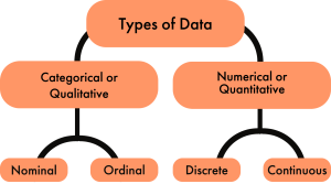
Qualitative Data

Categorical or qualitative data labels data into categories. Categorical data is defined in terms of natural language specifications. For example, name, sex, country of origin, are categories that represent qualitative data. There are two subcategories of qualitative data, nominal data and ordinal data.

Nominal Data

Ordinal Data

When the categories have a natural order, the categories are said to be ordinal . It can be ordered and measured. For example education level (H.S. diploma; 1 year certificate; 2 year degree; 4 year degree; masters degree; doctorate degree), satisfaction rating (extremely dislike; dislike; neutral; like; extremely like), etc. are categories that have a natural order to them. Ordinal data are commonly used for collecting demographic information (age, sex, race, etc.). This is particularly prevalent in marketing and insurance sectors, but it is also used by governments (e.g. the census), and is commonly used when conducting customer satisfaction surveys. Ordinal data is commonly represented using a bar graph .

Quantitative Data

Quantitative data has two subcategories, discrete data and continuous data.

Discrete Data

The data is discrete when the numbers do not touch each other on a real number line (e.g., 0, 1, 2, 3, 4…). Discrete data is whole numerical values typically shown as counts and contains only a finite number of possible values. For example, the number of visits to the doctor, the number of students in a class, etc. Discrete data is typically represented by a histogram .

Continuous Data

The data is continuous when it has an infinite number of possible values that can be selected within certain limits. (i.e., the numbers run into each other on a real number line). Continuous data is data that can be calculated . It has an infinite number of possible values that can be selected within certain limits. Examples of continuous data are temperature, time, height, etc. Continuous data is typically represented by a line graph .

Explore 1 – Types of data

Classify the data into qualitative or quantitative, then into a subcategory of nominal, ordinal, discrete or continuous.

Weight is a number that is measured and has order. It can also take on any number. So, weight is quantitative: continuous.

• egg size (small, medium, large, extra large)

Egg size is typically small, medium, large, or extra large that has a natural order. So, egg size is qualitative: ordinal.

• number of miles driven to work

Number of miles is a number that is measured and has order. It can also take on any number. So, number of miles is : quantitative: continuous.

• body temperature

Body temperature is a number that is measured and has order. It can also take on any number. So, temperature is quantitative: continuous.

• basketball team jersey number

Jersey numbers have no order and are numbers that are not measured. So, jersey number is qualitative: nominal.

• U.S. shoe size

Shoe size is a number. It is calculated based on a formula that includes the measure of your foot length. However, it has only whole or half numbers (e.g., 8 or 9.5). Shoe size has a natural order but has a finite number of options (e.g., half or whole numbers). So, shoe size is quantitative: discrete.

• military rank

Military rank is not numerical but is categorical with a natural order. So, military rank is qualitative: ordinal.

• university GPA

University GPA is a weighted average that is calculated, so it is quantitative: continuous.

Practice Exercises

• year of birth
• levels of fluency (language)
• height of players on a team
• dose of medicine
• political party
• course letter grades
• Quantitative: discrete
• Qualitative: ordinal
• Quantitative: continuous
• Qualitative: nominal

Types of Graphs and Charts

The type of graph or chart used to visualize data is determined by the type of data being represented. A pie chart or bar chart  is typically used for nominal data and a bar chart for ordinal data . For quantitative data , we typically use a histogram for discrete data and a line graph for continuous data .

A pie chart is a circular graphic which is divided into slices to illustrate numerical proportion. Pie charts are widely used in the business world and the mass media. The size of each slice is determined by the percentage represented by a category compared to the whole (i.e., the entire dataset). The percentage in each category adds to 100% or the whole.  

Explore 2 – Pie Charts

The pie chart shows the distribution of the Food and Drug Administration’s Budget of different programs for the fiscal year 2021. The total  budget was $6.1 billion. [1]

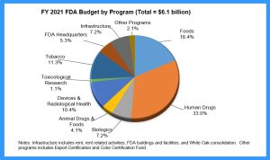
• How many categories are shown in the pie chart?

If we count the number of slices, there are 10 categories shown.

• What do the percentages represent?

The percentages show the percent of the $6.1 billion FDA budget that was spent on each category.

• Why is it vital to show the total budget on the chart?

Without the total budget we would be unable to calculate the amount spent on each category.

• Is there a limit to the number of categories that can be shown on a pie chart?

Yes. If the slices are too small to see, another method of representing the data should be used. Ideally, a pie chart should show no more than 5 or 6 categories.

• What does the largest slice represent?

The percentage of the total budget spent on human drugs.

• What does the smallest slice represent?

The percentage of the total budget spent on toxicological research.

• How could this pie chart be improved?

The slices could be ordered around the circle by size, and the 3-D look could be eliminated to avoid the distorted perspective and to make the graph clearer.

• Is this an appropriate use of a pie chart?

The chart is showing a comparison of all categories the budget went towards so it is appropriate.

Bar graphs are used to represent categorical data . Each category is represented as a bar either vertically or horizontally. A bar is the measured value or percentage of a category and there is equal space between each pair of consecutive bars. Bar graphs have the advantage of being easy to read and offer direct comparison of categories. 

Explore 3 – Bar Graphs

Graduation rates within 6 years from the first institution attended for first-time, full-time bachelor’s degree-seeking students at 4-year postsecondary institutions, by race/ethnicity: cohort entry year 2010.

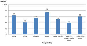
• How many categories are represented in the bar graph and what do they represent?

There are 7 categories representing the race/ethnicity of the students.

• What do the numbers above each bar represent and why may they be necessary?

The rounded percent of the category. They are necessary because it is very difficult to tell from the vertical scale the height of each bar.

• What does the tallest bar represent?

The percent of students who graduated within six years from their first institution within 6 years who were Asian.

• What does the shortest bar represent?

The percent of students who graduated within six years from their first institution within 6 years who were American Indian or Alaska Native.

• Is this an appropriate use of a bar graph?

Yes. The data is qualitative: nominal; there is no order within the categories.

Histograms are used to represent quantitative data that is discrete . A histogram divides up the range of possible values in a data set into classes or intervals. For each class, a rectangle is constructed with a base length equal to the range of values in that specific class and a length equal to the number of observations falling into that class. A histogram has an appearance similar to a vertical bar chart, but there are no gaps between the bars. The bars are ordered along the axis from the smallest to the largest possible value. Consequently, the bars cannot be reordered. Histograms are often used to illustrate the major features of the distribution of the data in a convenient form. They are also useful when dealing with large data sets (greater than 100 observations). They can help detect any unusual observations (outliers) or any gaps in the data.

Histograms may look similar to bar charts but they are really completely different. Histograms plot quantitative data with ranges of the data grouped into classes or intervals while bar charts plot categorical data. Histograms are used to show distributions while bar charts are used to compare categories. Bars can be reordered in bar charts but not in histograms. The bars of bar charts have the same width. The widths of the bars in a histogram need not be the same as long as the total area of all bars is one hundred percent if percentages are used or the total count, if counts are used. Therefore, values in bar graphs are given by the length of the bar while values in histograms are given by areas.

Explore 4 – Histograms

Reading data from a table can be less than enlightening and certainly doesn’t inspire much interest. Graphing the same data in a histogram gives a graphical representation where certain features are automatically highlighted.

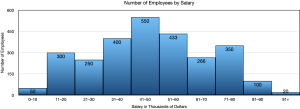
• What do you notice about the bars of this histogram compared to the bars of a bar graph?

The bars touch in a histogram but not in a bar chart. This is because the data is ordered along the axis.

• What do the numbers above the bars represent?

The number of employees whose salary lands in each class.

• State a feature of the graph that is very obvious to you.

Answers may vary. Very few employees make less than $10,000 or more than $91,000. $41,000 – $50,000 is the most common salary.

Line graphs are used when the data is quantitative and continuous . The axis acts as a real number line where every possible value is located. Line graphs are typically used to show how data values change over time.

Explore 5 – Line Graphs

Here is an example of a line graph.

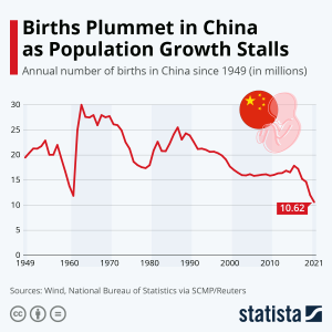
• What does this line graph represent?

Solution:  The number of annual births in China from 1949 to 2021.

• What do the numbers on the vertical axis represent?

Solution:  The number of births in millions.

• What do the numbers on the horizontal axis represent?

Solution:  The year.

• Is this an appropriate use of a line graph?

Solution:  Yes. The time scale in years is continuous and a line graph is appropriate for continuous data.

• Does a line graph highlight anything that a histogram may not?

Solution:  Yes. The trend in data over time. In this graph the trend of annual births is decreasing.

Infographics are often used by media outlets who are trying to tell a specific (often biased) story. They often combine charts or graphs with narrative and statistics.

Explore 6 – Infographics

Solution:  Since it is circular and based on percentages in each category, it is based on a pie chart.

• How many categories are represented?

Solution:  There are three categories.

• What story is the infographic trying to tell?

Solution:  About one third of Americans believe in aliens.

• How was the data gathered?

Solution:  A survey of 1522 U.S. adults.

• What does the largest blue area on the chart represent?

Solution:  The percentage of those surveyed that believe that all sightings can be explained by human activity or natural phenomena.

• What does the smallest grey area on the chart represent?

Solution:  The percentage of those surveyed that have no opinion on UFO sightings.

• Robert is involved in a group project for a class. The group has collected data to show the amount of time spent performing different tasks on a cell phone. The categories include making calls, Internet, text, music, videos, social media, email, games, and photos. What type of graph or chart should be used to display the average time spent per day on any of these tasks? Explain your reasoning.  
• A marketing firm wants to show what fraction of the overall market uses a particular Internet browser. What type of graph or chart should be used to display this information? Explain your reasoning.  
• The data is categorical so a bar graph should be used.
• The data is categorical. If there are not too many categories (browser used) then a pie chart would work since fraction of the market is used. Alternatively, a bar chart could be used showing the fraction or percent as the height of each bar.

• Name three (3) differences between a bar graph and a histogram.
• A bar graph is used for qualitative data while a histogram is used for quantitative data.
• In a bar graph the categories can be reordered. In a histogram the categories cannot be reordered.
• In a bar graph the bars do not touch. In a histogram the bars touch.
• A teacher wants to show their class the results of a midterm exam, without exposing any student names. What type of graph or chart should be used to display the scores earned on the midterm? Explain your reasoning.  
• A pizza company wants to display a graphic of the five favorite pizzas of their customers on the company website. What type of graph or chart should be used to display this information? Explain your reasoning.  
• Maria is keeping track of her daughter’s height by measuring her height on her birthday each year and recording it in a spreadsheet. What type of graph or chart should be used to display this information? Explain your reasoning
• Midterm scores may be quantitative as either raw scores or percentages, in which case they should show a histogram showing the number of students scoring in a given score (or percentage) interval. If the midterm results are letter grades, the data is qualitative but ordered. In this case, a pie chart could be used to show the percent of students with each letter grade, but it would be very busy.  A better option would be a bar graph showing the number of students at each letter grade.
• An infographic. This is categorical data so a (pizza) pie chart would be a good option or a bar chart.
• A line graph since the data is collected over time and time is continuous.

Perspectives

• Mike has collected data for a school project from a survey that asked, “What is your favorite pizza? ”. He surveyed 200 people and discovered that there were only 9 pizzas that were on the favorites list. In his report, he plans to show his data in a (pizza) pie chart. Is this the correct chart to use for his purpose? Explain your reasoning.  
• Sarah is keeping track of the value of her car every year. She started when she first bought the car new and looks up its value every year. She figures that when the car’s value drops to $5000, it is time for an upgrade. What type of graph or chart should be used to display this information? Explain your reasoning.  
• The Earth’s atmosphere is made up of 77% Nitrogen, 21% Oxygen, and 2% other gases. What type of graph or chart should be used to display this data? Explain your reasoning.  
• A pie chart could be used but with 9 categories there may be too many slices for the chart to be clear. A bar graph may be better due to the number of categories.
• A line graph since time is continuous and she will be able to see the trend in car value over time.
• The data is qualitative: nominal and has percentages that add to 100% so a pie chart would work well with only 3 categories. Alternatively, a bar chart would work.

Skills Exercises

• phone number
• https://www.fda.gov/about-fda/fda-basics/fact-sheet-fda-glance ↵

able to be put into categories

data that can be given labels and put into categories

qualitative data that can be put into labelled categories that have no order and no overlap

having nothing in common; no overlap

the number of times a data value has been recorded

a number or ratio expressed as a fraction of 100

a circular graphic which is divided into slices representing the number or percentage in each category

qualitative data that has a natural order

a graph where each category is represented by a vertical or horizontal bar that measures a frequency or percentage of the whole

expressed using a number or numbers

data that involves numerical values with order

data that is measured using whole numbers with only a finite number of possibilities

a graph similar in appearance to a vertical bar graph with gaps between the bars, ordered bars, with a bse length equal to the range of values in a specific class

data that has an infinite number of possible values that can be selected within certain limits

use arithmetic and the order of operations

a graph used for continuous data that uses an axis as a real number line where every possible value is located

a graphic showing a combination of graphs, charts, and statistics

Numeracy Copyright © 2023 by Utah Valley University is licensed under a Creative Commons Attribution-NonCommercial-ShareAlike 4.0 International License , except where otherwise noted.

Page Statistics

Table of contents.

• Introduction to Functional Computer
• Fundamentals of Architectural Design

Data Representation

• Instruction Set Architecture : Instructions and Formats
• Instruction Set Architecture : Design Models
• Instruction Set Architecture : Addressing Modes
• Performance Measurements and Issues
• Computer Architecture Assessment 1
• Fixed Point Arithmetic : Addition and Subtraction
• Fixed Point Arithmetic : Multiplication
• Fixed Point Arithmetic : Division
• Floating Point Arithmetic
• Arithmetic Logic Unit Design
• CPU's Data Path
• CPU's Control Unit
• Control Unit Design
• Concepts of Pipelining
• Computer Architecture Assessment 2
• Pipeline Hazards
• Memory Characteristics and Organization
• Cache Memory
• Virtual Memory
• I/O Communication and I/O Controller
• Input/Output Data Transfer
• Direct Memory Access controller and I/O Processor
• CPU Interrupts and Interrupt Handling
• Computer Architecture Assessment 3

Course Computer Architecture

Digital computers store and process information in binary form as digital logic has only two values "1" and "0" or in other words "True or False" or also said as "ON or OFF". This system is called radix 2. We human generally deal with radix 10 i.e. decimal. As a matter of convenience there are many other representations like Octal (Radix 8), Hexadecimal (Radix 16), Binary coded decimal (BCD), Decimal etc.

Every computer's CPU has a width measured in terms of bits such as 8 bit CPU, 16 bit CPU, 32 bit CPU etc. Similarly, each memory location can store a fixed number of bits and is called memory width. Given the size of the CPU and Memory, it is for the programmer to handle his data representation. Most of the readers may be knowing that 4 bits form a Nibble, 8 bits form a byte. The word length is defined by the Instruction Set Architecture of the CPU. The word length may be equal to the width of the CPU.

The memory simply stores information as a binary pattern of 1's and 0's. It is to be interpreted as what the content of a memory location means. If the CPU is in the Fetch cycle, it interprets the fetched memory content to be instruction and decodes based on Instruction format. In the Execute cycle, the information from memory is considered as data. As a common man using a computer, we think computers handle English or other alphabets, special characters or numbers. A programmer considers memory content to be data types of the programming language he uses. Now recall figure 1.2 and 1.3 of chapter 1 to reinforce your thought that conversion happens from computer user interface to internal representation and storage.

• Data Representation in Computers

Information handled by a computer is classified as instruction and data. A broad overview of the internal representation of the information is illustrated in figure 3.1. No matter whether it is data in a numeric or non-numeric form or integer, everything is internally represented in Binary. It is up to the programmer to handle the interpretation of the binary pattern and this interpretation is called Data Representation . These data representation schemes are all standardized by international organizations.

Choice of Data representation to be used in a computer is decided by

• The number types to be represented (integer, real, signed, unsigned, etc.)
• Range of values likely to be represented (maximum and minimum to be represented)
• The Precision of the numbers i.e. maximum accuracy of representation (floating point single precision, double precision etc)
• If non-numeric i.e. character, character representation standard to be chosen. ASCII, EBCDIC, UTF are examples of character representation standards.
• The hardware support in terms of word width, instruction.

Before we go into the details, let us take an example of interpretation. Say a byte in Memory has value "0011 0001". Although there exists a possibility of so many interpretations as in figure 3.2, the program has only one interpretation as decided by the programmer and declared in the program.

• Fixed point Number Representation

Fixed point numbers are also known as whole numbers or Integers. The number of bits used in representing the integer also implies the maximum number that can be represented in the system hardware. However for the efficiency of storage and operations, one may choose to represent the integer with one Byte, two Bytes, Four bytes or more. This space allocation is translated from the definition used by the programmer while defining a variable as integer short or long and the Instruction Set Architecture.

In addition to the bit length definition for integers, we also have a choice to represent them as below:

• Unsigned Integer : A positive number including zero can be represented in this format. All the allotted bits are utilised in defining the number. So if one is using 8 bits to represent the unsigned integer, the range of values that can be represented is 28 i.e. "0" to "255". If 16 bits are used for representing then the range is 216 i.e. "0 to 65535".
• Signed Integer : In this format negative numbers, zero, and positive numbers can be represented. A sign bit indicates the magnitude direction as positive or negative. There are three possible representations for signed integer and these are Sign Magnitude format, 1's Compliment format and 2's Complement format .

Signed Integer – Sign Magnitude format: Most Significant Bit (MSB) is reserved for indicating the direction of the magnitude (value). A "0" on MSB means a positive number and a "1" on MSB means a negative number. If n bits are used for representation, n-1 bits indicate the absolute value of the number. Examples for n=8:

Examples for n=8:

0010 1111 = + 47 Decimal (Positive number)

1010 1111 = - 47 Decimal (Negative Number)

0111 1110 = +126 (Positive number)

1111 1110 = -126 (Negative Number)

0000 0000 = + 0 (Postive Number)

1000 0000 = - 0 (Negative Number)

Although this method is easy to understand, Sign Magnitude representation has several shortcomings like

• Zero can be represented in two ways causing redundancy and confusion.
• The total range for magnitude representation is limited to 2n-1, although n bits were accounted.
• The separate sign bit makes the addition and subtraction more complicated. Also, comparing two numbers is not straightforward.

Signed Integer – 1’s Complement format: In this format too, MSB is reserved as the sign bit. But the difference is in representing the Magnitude part of the value for negative numbers (magnitude) is inversed and hence called 1’s Complement form. The positive numbers are represented as it is in binary. Let us see some examples to better our understanding.

1101 0000 = - 47 Decimal (Negative Number)

1000 0001 = -126 (Negative Number)

1111 1111 = - 0 (Negative Number)

• Converting a given binary number to its 2's complement form

Step 1 . -x = x' + 1 where x' is the one's complement of x.

Step 2 Extend the data width of the number, fill up with sign extension i.e. MSB bit is used to fill the bits.

Example: -47 decimal over 8bit representation

As you can see zero is not getting represented with redundancy. There is only one way of representing zero. The other problem of the complexity of the arithmetic operation is also eliminated in 2’s complement representation. Subtraction is done as Addition.

More exercises on number conversion are left to the self-interest of readers.

• Floating Point Number system

The maximum number at best represented as a whole number is 2 n . In the Scientific world, we do come across numbers like Mass of an Electron is 9.10939 x 10-31 Kg. Velocity of light is 2.99792458 x 108 m/s. Imagine to write the number in a piece of paper without exponent and converting into binary for computer representation. Sure you are tired!!. It makes no sense to write a number in non- readable form or non- processible form. Hence we write such large or small numbers using exponent and mantissa. This is said to be Floating Point representation or real number representation. he real number system could have infinite values between 0 and 1.

Representation in computer

Unlike the two's complement representation for integer numbers, Floating Point number uses Sign and Magnitude representation for both mantissa and exponent . In the number 9.10939 x 1031, in decimal form, +31 is Exponent, 9.10939 is known as Fraction . Mantissa, Significand and fraction are synonymously used terms. In the computer, the representation is binary and the binary point is not fixed. For example, a number, say, 23.345 can be written as 2.3345 x 101 or 0.23345 x 102 or 2334.5 x 10-2. The representation 2.3345 x 101 is said to be in normalised form.

Floating-point numbers usually use multiple words in memory as we need to allot a sign bit, few bits for exponent and many bits for mantissa. There are standards for such allocation which we will see sooner.

• IEEE 754 Floating Point Representation

We have two standards known as Single Precision and Double Precision from IEEE. These standards enable portability among different computers. Figure 3.3 picturizes Single precision while figure 3.4 picturizes double precision. Single Precision uses 32bit format while double precision is 64 bits word length. As the name suggests double precision can represent fractions with larger accuracy. In both the cases, MSB is sign bit for the mantissa part, followed by Exponent and Mantissa. The exponent part has its sign bit.

It is to be noted that in Single Precision, we can represent an exponent in the range -127 to +127. It is possible as a result of arithmetic operations the resulting exponent may not fit in. This situation is called overflow in the case of positive exponent and underflow in the case of negative exponent. The Double Precision format has 11 bits for exponent meaning a number as large as -1023 to 1023 can be represented. The programmer has to make a choice between Single Precision and Double Precision declaration using his knowledge about the data being handled.

The Floating Point operations on the regular CPU is very very slow. Generally, a special purpose CPU known as Co-processor is used. This Co-processor works in tandem with the main CPU. The programmer should be using the float declaration only if his data is in real number form. Float declaration is not to be used generously.

• Decimal Numbers Representation

Decimal numbers (radix 10) are represented and processed in the system with the support of additional hardware. We deal with numbers in decimal format in everyday life. Some machines implement decimal arithmetic too, like floating-point arithmetic hardware. In such a case, the CPU uses decimal numbers in BCD (binary coded decimal) form and does BCD arithmetic operation. BCD operates on radix 10. This hardware operates without conversion to pure binary. It uses a nibble to represent a number in packed BCD form. BCD operations require not only special hardware but also decimal instruction set.

• Exceptions and Error Detection

All of us know that when we do arithmetic operations, we get answers which have more digits than the operands (Ex: 8 x 2= 16). This happens in computer arithmetic operations too. When the result size exceeds the allotted size of the variable or the register, it becomes an error and exception. The exception conditions associated with numbers and number operations are Overflow, Underflow, Truncation, Rounding and Multiple Precision . These are detected by the associated hardware in arithmetic Unit. These exceptions apply to both Fixed Point and Floating Point operations. Each of these exceptional conditions has a flag bit assigned in the Processor Status Word (PSW). We may discuss more in detail in the later chapters.

• Character Representation

Another data type is non-numeric and is largely character sets. We use a human-understandable character set to communicate with computer i.e. for both input and output. Standard character sets like EBCDIC and ASCII are chosen to represent alphabets, numbers and special characters. Nowadays Unicode standard is also in use for non-English language like Chinese, Hindi, Spanish, etc. These codes are accessible and available on the internet. Interested readers may access and learn more.

1. Track your progress [Earn 200 points]

Mark as complete

2. Provide your ratings to this chapter [Earn 100 points]

• school Campus Bookshelves
• menu_book Bookshelves
• perm_media Learning Objects
• login Login
• how_to_reg Request Instructor Account
• hub Instructor Commons
• Download Page (PDF)
• Download Full Book (PDF)
• Periodic Table
• Physics Constants
• Scientific Calculator
• Reference & Cite
• Tools expand_more
• Readability

selected template will load here

This action is not available.

2: Graphical Representations of Data

• Last updated
• Save as PDF
• Page ID 22222

In this chapter, you will study numerical and graphical ways to describe and display your data. This area of statistics is called "Descriptive Statistics." You will learn how to calculate, and even more importantly, how to interpret these measurements and graphs.

• 2.1: Introduction In this chapter, you will study numerical and graphical ways to describe and display your data. This area of statistics is called "Descriptive Statistics." You will learn how to calculate, and even more importantly, how to interpret these measurements and graphs. In this chapter, we will briefly look at stem-and-leaf plots, line graphs, and bar graphs, as well as frequency polygons, and time series graphs. Our emphasis will be on histograms and box plots.
• 2.2: Stem-and-Leaf Graphs (Stemplots), Line Graphs, and Bar Graphs A stem-and-leaf plot is a way to plot data and look at the distribution, where all data values within a class are visible. The advantage in a stem-and-leaf plot is that all values are listed, unlike a histogram, which gives classes of data values. A line graph is often used to represent a set of data values in which a quantity varies with time. These graphs are useful for finding trends.  A bar graph is a chart that uses either horizontal or vertical bars to show comparisons among categories.
• 2.3: Histograms, Frequency Polygons, and Time Series Graphs A histogram is a graphic version of a frequency distribution. The graph consists of bars of equal width drawn adjacent to each other. The horizontal scale represents classes of quantitative data values and the vertical scale represents frequencies. The heights of the bars correspond to frequency values. Histograms are typically used for large, continuous, quantitative data sets. A frequency polygon can also be used when graphing large data sets with data points that repeat.
• 2.4: Using Excel to Create Graphs Using technology to create graphs will make the graphs faster to create, more precise, and give the ability to use larger amounts of data. This section focuses on using Excel to create graphs.
• 2.5: Graphs that Deceive It's common to see graphs displayed in a misleading manner in social media and other instances. This could be done purposefully to make a point, or it could be accidental. Either way, it's important to recognize these instances to ensure you are not misled.
• 2.E: Graphical Representations of Data (Exercises) These are homework exercises to accompany the Textmap created for "Introductory Statistics" by OpenStax.

Contributors and Attributions

Barbara Illowsky and Susan Dean (De Anza College) with many other contributing authors. Content produced by OpenStax College is licensed under a Creative Commons Attribution License 4.0 license. Download for free at http://cnx.org/contents/[email protected] .

• Data representation

Bytes of memory

• Abstract machine

Unsigned integer representation

Signed integer representation, pointer representation, array representation, compiler layout, array access performance, collection representation.

• Consequences of size and alignment rules

Uninitialized objects

Pointer arithmetic, undefined behavior.

• Computer arithmetic

Arena allocation

This course is about learning how computers work, from the perspective of systems software: what makes programs work fast or slow, and how properties of the machines we program impact the programs we write. We want to communicate ideas, tools, and an experimental approach.

The course divides into six units:

• Assembly & machine programming
• Storage & caching
• Kernel programming
• Process management
• Concurrency

The first unit, data representation , is all about how different forms of data can be represented in terms the computer can understand.

Computer memory is kind of like a Lite Brite.

A Lite Brite is big black backlit pegboard coupled with a supply of colored pegs, in a limited set of colors. You can plug in the pegs to make all kinds of designs. A computer’s memory is like a vast pegboard where each slot holds one of 256 different colors. The colors are numbered 0 through 255, so each slot holds one byte . (A byte is a number between 0 and 255, inclusive.)

A slot of computer memory is identified by its address . On a computer with M bytes of memory, and therefore M slots, you can think of the address as a number between 0 and M −1. My laptop has 16 gibibytes of memory, so M = 16×2 30 = 2 34 = 17,179,869,184 = 0x4'0000'0000 —a very large number!

The problem of data representation is the problem of representing all the concepts we might want to use in programming—integers, fractions, real numbers, sets, pictures, texts, buildings, animal species, relationships—using the limited medium of addresses and bytes.

Powers of ten and powers of two. Digital computers love the number two and all powers of two. The electronics of digital computers are based on the bit , the smallest unit of storage, which a base-two digit: either 0 or 1. More complicated objects are represented by collections of bits. This choice has many scale and error-correction advantages. It also refracts upwards to larger choices, and even into terminology. Memory chips, for example, have capacities based on large powers of two, such as 2 30 bytes. Since 2 10 = 1024 is pretty close to 1,000, 2 20 = 1,048,576 is pretty close to a million, and 2 30 = 1,073,741,824 is pretty close to a billion, it’s common to refer to 2 30 bytes of memory as “a giga byte,” even though that actually means 10 9 = 1,000,000,000 bytes. But for greater precision, there are terms that explicitly signal the use of powers of two. 2 30 is a gibibyte : the “-bi-” component means “binary.”

Virtual memory. Modern computers actually abstract their memory spaces using a technique called virtual memory . The lowest-level kind of address, called a physical address , really does take on values between 0 and M −1. However, even on a 16GiB machine like my laptop, the addresses we see in programs can take on values like 0x7ffe'ea2c'aa67 that are much larger than M −1 = 0x3'ffff'ffff . The addresses used in programs are called virtual addresses . They’re incredibly useful for protection: since different running programs have logically independent address spaces, it’s much less likely that a bug in one program will crash the whole machine. We’ll learn about virtual memory in much more depth in the kernel unit ; the distinction between virtual and physical addresses is not as critical for data representation.

Most programming languages prevent their users from directly accessing memory. But not C and C++! These languages let you access any byte of memory with a valid address. This is powerful; it is also very dangerous. But it lets us get a hands-on view of how computers really work.

C++ programs accomplish their work by constructing, examining, and modifying objects . An object is a region of data storage that contains a value, such as the integer 12. (The standard specifically says “a region of data storage in the execution environment, the contents of which can represent values”.) Memory is called “memory” because it remembers object values.

In this unit, we often use functions called hexdump to examine memory. These functions are defined in hexdump.cc . hexdump_object(x) prints out the bytes of memory that comprise an object named x , while hexdump(ptr, size) prints out the size bytes of memory starting at a pointer ptr .

For example, in datarep1/add.cc , we might use hexdump_object to examine the memory used to represent some integers:

This display reports that a , b , and c are each four bytes long; that a , b , and c are located at different, nonoverlapping addresses (the long hex number in the first column); and shows us how the numbers 1, 2, and 3 are represented in terms of bytes. (More on that later.)

The compiler, hardware, and standard together define how objects of different types map to bytes. Each object uses a contiguous range of addresses (and thus bytes), and objects never overlap (objects that are active simultaneously are always stored in distinct address ranges).

Since C and C++ are designed to help software interface with hardware devices, their standards are transparent about how objects are stored. A C++ program can ask how big an object is using the sizeof keyword. sizeof(T) returns the number of bytes in the representation of an object of type T , and sizeof(x) returns the size of object x . The result of sizeof is a value of type size_t , which is an unsigned integer type large enough to hold any representable size. On 64-bit architectures, such as x86-64 (our focus in this course), size_t can hold numbers between 0 and 2 64 –1.

Qualitatively different objects may have the same data representation. For example, the following three objects have the same data representation on x86-64, which you can verify using hexdump :

In C and C++, you can’t reliably tell the type of an object by looking at the contents of its memory. That’s why tricks like our different addf*.cc functions work.

An object can have many names. For example, here, local and *ptr refer to the same object:

The different names for an object are sometimes called aliases .

There are five objects here:

• ch1 , a global variable
• ch2 , a constant (non-modifiable) global variable
• ch3 , a local variable
• ch4 , a local variable
• the anonymous storage allocated by new char and accessed by *ch4

Each object has a lifetime , which is called storage duration by the standard. There are three different kinds of lifetime.

• static lifetime: The object lasts as long as the program runs. ( ch1 , ch2 )
• automatic lifetime: The compiler allocates and destroys the object automatically as the program runs, based on the object’s scope (the region of the program in which it is meaningful). ( ch3 , ch4 )
• dynamic lifetime: The programmer allocates and destroys the object explicitly. ( *allocated_ch )

Objects with dynamic lifetime aren’t easy to use correctly. Dynamic lifetime causes many serious problems in C programs, including memory leaks, use-after-free, double-free, and so forth. Those serious problems cause undefined behavior and play a “disastrously central role” in “our ongoing computer security nightmare” . But dynamic lifetime is critically important. Only with dynamic lifetime can you construct an object whose size isn’t known at compile time, or construct an object that outlives the function that created it.

The compiler and operating system work together to put objects at different addresses. A program’s address space (which is the range of addresses accessible to a program) divides into regions called segments . Objects with different lifetimes are placed into different segments. The most important segments are:

• Code (also known as text or read-only data ). Contains instructions and constant global objects. Unmodifiable; static lifetime.
• Data . Contains non-constant global objects. Modifiable; static lifetime.
• Heap . Modifiable; dynamic lifetime.
• Stack . Modifiable; automatic lifetime.

The compiler decides on a segment for each object based on its lifetime. The final compiler phase, which is called the linker , then groups all the program’s objects by segment (so, for instance, global variables from different compiler runs are grouped together into a single segment). Finally, when a program runs, the operating system loads the segments into memory. (The stack and heap segments grow on demand.)

We can use a program to investigate where objects with different lifetimes are stored. (See cs61-lectures/datarep2/mexplore0.cc .) This shows address ranges like this:

Constant global data and global data have the same lifetime, but are stored in different segments. The operating system uses different segments so it can prevent the program from modifying constants. It marks the code segment, which contains functions (instructions) and constant global data, as read-only, and any attempt to modify code-segment memory causes a crash (a “Segmentation violation”).

An executable is normally at least as big as the static-lifetime data (the code and data segments together). Since all that data must be in memory for the entire lifetime of the program, it’s written to disk and then loaded by the OS before the program starts running. There is an exception, however: the “bss” segment is used to hold modifiable static-lifetime data with initial value zero. Such data is common, since all static-lifetime data is initialized to zero unless otherwise specified in the program text. Rather than storing a bunch of zeros in the object files and executable, the compiler and linker simply track the location and size of all zero-initialized global data. The operating system sets this memory to zero during the program load process. Clearing memory is faster than loading data from disk, so this optimization saves both time (the program loads faster) and space (the executable is smaller).

Abstract machine and hardware

Programming involves turning an idea into hardware instructions. This transformation happens in multiple steps, some you control and some controlled by other programs.

First you have an idea , like “I want to make a flappy bird iPhone game.” The computer can’t (yet) understand that idea. So you transform the idea into a program , written in some programming language . This process is called programming.

A C++ program actually runs on an abstract machine . The behavior of this machine is defined by the C++ standard , a technical document. This document is supposed to be so precisely written as to have an exact mathematical meaning, defining exactly how every C++ program behaves. But the document can’t run programs!

C++ programs run on hardware (mostly), and the hardware determines what behavior we see. Mapping abstract machine behavior to instructions on real hardware is the task of the C++ compiler (and the standard library and operating system). A C++ compiler is correct if and only if it translates each correct program to instructions that simulate the expected behavior of the abstract machine.

This same rough series of transformations happens for any programming language, although some languages use interpreters rather than compilers.

A bit is the fundamental unit of digital information: it’s either 0 or 1.

C++ manages memory in units of bytes —8 contiguous bits that together can represent numbers between 0 and 255. C’s unit for a byte is char : the abstract machine says a byte is stored in char . That means an unsigned char holds values in the inclusive range [0, 255].

The C++ standard actually doesn’t require that a byte hold 8 bits, and on some crazy machines from decades ago , bytes could hold nine bits! (!?)

But larger numbers, such as 258, don’t fit in a single byte. To represent such numbers, we must use multiple bytes. The abstract machine doesn’t specify exactly how this is done—it’s the compiler and hardware’s job to implement a choice. But modern computers always use place–value notation , just like in decimal numbers. In decimal, the number 258 is written with three digits, the meanings of which are determined both by the digit and by their place in the overall number:

\[ 258 = 2\times10^2 + 5\times10^1 + 8\times10^0 \]

The computer uses base 256 instead of base 10. Two adjacent bytes can represent numbers between 0 and \(255\times256+255 = 65535 = 2^{16}-1\) , inclusive. A number larger than this would take three or more bytes.

\[ 258 = 1\times256^1 + 2\times256^0 \]

On x86-64, the ones place, the least significant byte, is on the left, at the lowest address in the contiguous two-byte range used to represent the integer. This is the opposite of how decimal numbers are written: decimal numbers put the most significant digit on the left. The representation choice of putting the least-significant byte in the lowest address is called little-endian representation. x86-64 uses little-endian representation.

Some computers actually store multi-byte integers the other way, with the most significant byte stored in the lowest address; that’s called big-endian representation. The Internet’s fundamental protocols, such as IP and TCP, also use big-endian order for multi-byte integers, so big-endian is also called “network” byte order.

The C++ standard defines five fundamental unsigned integer types, along with relationships among their sizes. Here they are, along with their actual sizes and ranges on x86-64:

Other architectures and operating systems implement different ranges for these types. For instance, on IA32 machines like Intel’s Pentium (the 32-bit processors that predated x86-64), sizeof(long) was 4, not 8.

Note that all values of a smaller unsigned integer type can fit in any larger unsigned integer type. When a value of a larger unsigned integer type is placed in a smaller unsigned integer object, however, not every value fits; for instance, the unsigned short value 258 doesn’t fit in an unsigned char x . When this occurs, the C++ abstract machine requires that the smaller object’s value equals the least -significant bits of the larger value (so x will equal 2).

In addition to these types, whose sizes can vary, C++ has integer types whose sizes are fixed. uint8_t , uint16_t , uint32_t , and uint64_t define 8-bit, 16-bit, 32-bit, and 64-bit unsigned integers, respectively; on x86-64, these correspond to unsigned char , unsigned short , unsigned int , and unsigned long .

This general procedure is used to represent a multi-byte integer in memory.

• Write the large integer in hexadecimal format, including all leading zeros required by the type size. For example, the unsigned value 65534 would be written 0x0000FFFE . There will be twice as many hexadecimal digits as sizeof(TYPE) .
• Divide the integer into its component bytes, which are its digits in base 256. In our example, they are, from most to least significant, 0x00, 0x00, 0xFF, and 0xFE.

In little-endian representation, the bytes are stored in memory from least to most significant. If our example was stored at address 0x30, we would have:

In big-endian representation, the bytes are stored in the reverse order.

Computers are often fastest at dealing with fixed-length numbers, rather than variable-length numbers, and processor internals are organized around a fixed word size . A word is the natural unit of data used by a processor design . In most modern processors, this natural unit is 8 bytes or 64 bits , because this is the power-of-two number of bytes big enough to hold those processors’ memory addresses. Many older processors could access less memory and had correspondingly smaller word sizes, such as 4 bytes (32 bits).

The best representation for signed integers—and the choice made by x86-64, and by the C++20 abstract machine—is two’s complement . Two’s complement representation is based on this principle: Addition and subtraction of signed integers shall use the same instructions as addition and subtraction of unsigned integers.

To see what this means, let’s think about what -x should mean when x is an unsigned integer. Wait, negative unsigned?! This isn’t an oxymoron because C++ uses modular arithmetic for unsigned integers: the result of an arithmetic operation on unsigned values is always taken modulo 2 B , where B is the number of bits in the unsigned value type. Thus, on x86-64,

-x is simply the number that, when added to x , yields 0 (mod 2 B ). For example, when unsigned x = 0xFFFFFFFFU , then -x == 1U , since x + -x equals zero (mod 2 32 ).

To obtain -x , we flip all the bits in x (an operation written ~x ) and then add 1. To see why, consider the bit representations. What is x + (~x + 1) ? Well, (~x) i (the i th bit of ~x ) is 1 whenever x i is 0, and vice versa. That means that every bit of x + ~x is 1 (there are no carries), and x + ~x is the largest unsigned integer, with value 2 B -1. If we add 1 to this, we get 2 B . Which is 0 (mod 2 B )! The highest “carry” bit is dropped, leaving zero.

Two’s complement arithmetic uses half of the unsigned integer representations for negative numbers. A two’s-complement signed integer with B bits has the following values:

• If the most-significant bit is 1, the represented number is negative. Specifically, the represented number is – (~x + 1) , where the outer negative sign is mathematical negation (not computer arithmetic).
• If every bit is 0, the represented number is 0.
• If the most-significant but is 0 but some other bit is 1, the represented number is positive.

The most significant bit is also called the sign bit , because if it is 1, then the represented value depends on the signedness of the type (and that value is negative for signed types).

Another way to think about two’s-complement is that, for B -bit integers, the most-significant bit has place value 2 B –1 in unsigned arithmetic and negative 2 B –1 in signed arithmetic. All other bits have the same place values in both kinds of arithmetic.

The two’s-complement bit pattern for x + y is the same whether x and y are considered as signed or unsigned values. For example, in 4-bit arithmetic, 5 has representation 0b0101 , while the representation 0b1100 represents 12 if unsigned and –4 if signed ( ~0b1100 + 1 = 0b0011 + 1 == 4). Let’s add those bit patterns and see what we get:

Note that this is the right answer for both signed and unsigned arithmetic : 5 + 12 = 17 = 1 (mod 16), and 5 + -4 = 1.

Subtraction and multiplication also produce the same results for unsigned arithmetic and signed two’s-complement arithmetic. (For instance, 5 * 12 = 60 = 12 (mod 16), and 5 * -4 = -20 = -4 (mod 16).) This is not true of division. (Consider dividing the 4-bit representation 0b1110 by 2. In signed arithmetic, 0b1110 represents -2, so 0b1110/2 == 0b1111 (-1); but in unsigned arithmetic, 0b1110 is 14, so 0b1110/2 == 0b0111 (7).) And, of course, it is not true of comparison. In signed 4-bit arithmetic, 0b1110 < 0 , but in unsigned 4-bit arithmetic, 0b1110 > 0 . This means that a C compiler for a two’s-complement machine can use a single add instruction for either signed or unsigned numbers, but it must generate different instruction patterns for signed and unsigned division (or less-than, or greater-than).

There are a couple quirks with C signed arithmetic. First, in two’s complement, there are more negative numbers than positive numbers. A representation with sign bit is 1, but every other bit 0, has no positive counterpart at the same bit width: for this number, -x == x . (In 4-bit arithmetic, -0b1000 == ~0b1000 + 1 == 0b0111 + 1 == 0b1000 .) Second, and far worse, is that arithmetic overflow on signed integers is undefined behavior .

The C++ abstract machine requires that signed integers have the same sizes as their unsigned counterparts.

We distinguish pointers , which are concepts in the C abstract machine, from addresses , which are hardware concepts. A pointer combines an address and a type.

The memory representation of a pointer is the same as the representation of its address value. The size of that integer is the machine’s word size; for example, on x86-64, a pointer occupies 8 bytes, and a pointer to an object located at address 0x400abc would be stored as:

The C++ abstract machine defines an unsigned integer type uintptr_t that can hold any address. (You have to #include <inttypes.h> or <cinttypes> to get the definition.) On most machines, including x86-64, uintptr_t is the same as unsigned long . Cast a pointer to an integer address value with syntax like (uintptr_t) ptr ; cast back to a pointer with syntax like (T*) addr . Casts between pointer types and uintptr_t are information preserving, so this assertion will never fail:

Since it is a 64-bit architecture, the size of an x86-64 address is 64 bits (8 bytes). That’s also the size of x86-64 pointers.

To represent an array of integers, C++ and C allocate the integers next to each other in memory, in sequential addresses, with no gaps or overlaps. Here, we put the integers 0, 1, and 258 next to each other, starting at address 1008:

Say that you have an array of N integers, and you access each of those integers in order, accessing each integer exactly once. Does the order matter?

Computer memory is random-access memory (RAM), which means that a program can access any bytes of memory in any order—it’s not, for example, required to read memory in ascending order by address. But if we run experiments, we can see that even in RAM, different access orders have very different performance characteristics.

Our arraysum program sums up all the integers in an array of N integers, using an access order based on its arguments, and prints the resulting delay. Here’s the result of a couple experiments on accessing 10,000,000 items in three orders, “up” order (sequential: elements 0, 1, 2, 3, …), “down” order (reverse sequential: N , N −1, N −2, …), and “random” order (as it sounds).

Wow! Down order is just a bit slower than up, but random order seems about 40 times slower. Why?

Random order is defeating many of the internal architectural optimizations that make memory access fast on modern machines. Sequential order, since it’s more predictable, is much easier to optimize.

Foreshadowing. This part of the lecture is a teaser for the Storage unit, where we cover access patterns and caching, including the processor caches that explain this phenomenon, in much more depth.

The C++ programming language offers several collection mechanisms for grouping subobjects together into new kinds of object. The collections are arrays, structs, and unions. (Classes are a kind of struct. All library types, such as vectors, lists, and hash tables, use combinations of these collection types.) The abstract machine defines how subobjects are laid out inside a collection. This is important, because it lets C/C++ programs exchange messages with hardware and even with programs written in other languages: messages can be exchanged only when both parties agree on layout.

Array layout in C++ is particularly simple: The objects in an array are laid out sequentially in memory, with no gaps or overlaps. Assume a declaration like T x[N] , where x is an array of N objects of type T , and say that the address of x is a . Then the address of element x[i] equals a + i * sizeof(T) , and sizeof(a) == N * sizeof(T) .

Sidebar: Vector representation

The C++ library type std::vector defines an array that can grow and shrink. For instance, this function creates a vector containing the numbers 0 up to N in sequence:

Here, v is an object with automatic lifetime. This means its size (in the sizeof sense) is fixed at compile time. Remember that the sizes of static- and automatic-lifetime objects must be known at compile time; only dynamic-lifetime objects can have varying size based on runtime parameters. So where and how are v ’s contents stored?

The C++ abstract machine requires that v ’s elements are stored in an array in memory. (The v.data() method returns a pointer to the first element of the array.) But it does not define std::vector ’s layout otherwise, and C++ library designers can choose different layouts based on their needs. We found these to hold for the std::vector in our library:

sizeof(v) == 24 for any vector of any type, and the address of v is a stack address (i.e., v is located in the stack segment).

The first 8 bytes of the vector hold the address of the first element of the contents array—call it the begin address . This address is a heap address, which is as expected, since the contents must have dynamic lifetime. The value of the begin address is the same as that of v.data() .

Bytes 8–15 hold the address just past the contents array—call it the end address . Its value is the same as &v.data()[v.size()] . If the vector is empty, then the begin address and the end address are the same.

Bytes 16–23 hold an address greater than or equal to the end address. This is the capacity address . As a vector grows, it will sometimes outgrow its current location and move its contents to new memory addresses. To reduce the number of copies, vectors usually to request more memory from the operating system than they immediately need; this additional space, which is called “capacity,” supports cheap growth. Often the capacity doubles on each growth spurt, since this allows operations like v.push_back() to execute in O (1) time on average.

Compilers must also decide where different objects are stored when those objects are not part of a collection. For instance, consider this program:

The abstract machine says these objects cannot overlap, but does not otherwise constrain their positions in memory.

On Linux, GCC will put all these variables into the stack segment, which we can see using hexdump . But it can put them in the stack segment in any order , as we can see by reordering the declarations (try declaration order i1 , c1 , i2 , c2 , c3 ), by changing optimization levels, or by adding different scopes (braces). The abstract machine gives the programmer no guarantees about how object addresses relate. In fact, the compiler may move objects around during execution, as long as it ensures that the program behaves according to the abstract machine. Modern optimizing compilers often do this, particularly for automatic objects.

But what order does the compiler choose? With optimization disabled, the compiler appears to lay out objects in decreasing order by declaration, so the first declared variable in the function has the highest address. With optimization enabled, the compiler follows roughly the same guideline, but it also rearranges objects by type—for instance, it tends to group char s together—and it can reuse space if different variables in the same function have disjoint lifetimes. The optimizing compiler tends to use less space for the same set of variables. This is because it’s arranging objects by alignment.

The C++ compiler and library restricts the addresses at which some kinds of data appear. In particular, the address of every int value is always a multiple of 4, whether it’s located on the stack (automatic lifetime), the data segment (static lifetime), or the heap (dynamic lifetime).

A bunch of observations will show you these rules:

These are the alignment restrictions for an x86-64 Linux machine.

These restrictions hold for most x86-64 operating systems, except that on Windows, the long type has size and alignment 4. (The long long type has size and alignment 8 on all x86-64 operating systems.)

Just like every type has a size, every type has an alignment. The alignment of a type T is a number a ≥1 such that the address of every object of type T must be a multiple of a . Every object with type T has size sizeof(T) —it occupies sizeof(T) contiguous bytes of memory; and has alignment alignof(T) —the address of its first byte is a multiple of alignof(T) . You can also say sizeof(x) and alignof(x) where x is the name of an object or another expression.

Alignment restrictions can make hardware simpler, and therefore faster. For instance, consider cache blocks. CPUs access memory through a transparent hardware cache. Data moves from primary memory, or RAM (which is large—a couple gigabytes on most laptops—and uses cheaper, slower technology) to the cache in units of 64 or 128 bytes. Those units are always aligned: on a machine with 128-byte cache blocks, the bytes with memory addresses [127, 128, 129, 130] live in two different cache blocks (with addresses [0, 127] and [128, 255]). But the 4 bytes with addresses [4n, 4n+1, 4n+2, 4n+3] always live in the same cache block. (This is true for any small power of two: the 8 bytes with addresses [8n,…,8n+7] always live in the same cache block.) In general, it’s often possible to make a system faster by leveraging restrictions—and here, the CPU hardware can load data faster when it can assume that the data lives in exactly one cache line.

The compiler, library, and operating system all work together to enforce alignment restrictions.

On x86-64 Linux, alignof(T) == sizeof(T) for all fundamental types (the types built in to C: integer types, floating point types, and pointers). But this isn’t always true; on x86-32 Linux, double has size 8 but alignment 4.

It’s possible to construct user-defined types of arbitrary size, but the largest alignment required by a machine is fixed for that machine. C++ lets you find the maximum alignment for a machine with alignof(std::max_align_t) ; on x86-64, this is 16, the alignment of the type long double (and the alignment of some less-commonly-used SIMD “vector” types ).

We now turn to the abstract machine rules for laying out all collections. The sizes and alignments for user-defined types—arrays, structs, and unions—are derived from a couple simple rules or principles. Here they are. The first rule applies to all types.

1. First-member rule. The address of the first member of a collection equals the address of the collection.

Thus, the address of an array is the same as the address of its first element. The address of a struct is the same as the address of the first member of the struct.

The next three rules depend on the class of collection. Every C abstract machine enforces these rules.

2. Array rule. Arrays are laid out sequentially as described above.

3. Struct rule. The second and subsequent members of a struct are laid out in order, with no overlap, subject to alignment constraints.

4. Union rule. All members of a union share the address of the union.

In C, every struct follows the struct rule, but in C++, only simple structs follow the rule. Complicated structs, such as structs with some public and some private members, or structs with virtual functions, can be laid out however the compiler chooses. The typical situation is that C++ compilers for a machine architecture (e.g., “Linux x86-64”) will all agree on a layout procedure for complicated structs. This allows code compiled by different compilers to interoperate.

That next rule defines the operation of the malloc library function.

5. Malloc rule. Any non-null pointer returned by malloc has alignment appropriate for any type. In other words, assuming the allocated size is adequate, the pointer returned from malloc can safely be cast to T* for any T .

Oddly, this holds even for small allocations. The C++ standard (the abstract machine) requires that malloc(1) return a pointer whose alignment is appropriate for any type, including types that don’t fit.

And the final rule is not required by the abstract machine, but it’s how sizes and alignments on our machines work.

6. Minimum rule. The sizes and alignments of user-defined types, and the offsets of struct members, are minimized within the constraints of the other rules.

The minimum rule, and the sizes and alignments of basic types, are defined by the x86-64 Linux “ABI” —its Application Binary Interface. This specification standardizes how x86-64 Linux C compilers should behave, and lets users mix and match compilers without problems.

Consequences of the size and alignment rules

From these rules we can derive some interesting consequences.

First, the size of every type is a multiple of its alignment .

To see why, consider an array with two elements. By the array rule, these elements have addresses a and a+sizeof(T) , where a is the address of the array. Both of these addresses contain a T , so they are both a multiple of alignof(T) . That means sizeof(T) is also a multiple of alignof(T) .

We can also characterize the sizes and alignments of different collections .

• The size of an array of N elements of type T is N * sizeof(T) : the sum of the sizes of its elements. The alignment of the array is alignof(T) .
• The size of a union is the maximum of the sizes of its components (because the union can only hold one component at a time). Its alignment is also the maximum of the alignments of its components.
• The size of a struct is at least as big as the sum of the sizes of its components. Its alignment is the maximum of the alignments of its components.

Thus, the alignment of every collection equals the maximum of the alignments of its components.

It’s also true that the alignment equals the least common multiple of the alignments of its components. You might have thought lcm was a better answer, but the max is the same as the lcm for every architecture that matters, because all fundamental alignments are powers of two.

The size of a struct might be larger than the sum of the sizes of its components, because of alignment constraints. Since the compiler must lay out struct components in order, and it must obey the components’ alignment constraints, and it must ensure different components occupy disjoint addresses, it must sometimes introduce extra space in structs. Here’s an example: the struct will have 3 bytes of padding after char c , to ensure that int i2 has the correct alignment.

Thanks to padding, reordering struct components can sometimes reduce the total size of a struct. Padding can happen at the end of a struct as well as the middle. Padding can never happen at the start of a struct, however (because of Rule 1).

The rules also imply that the offset of any struct member —which is the difference between the address of the member and the address of the containing struct— is a multiple of the member’s alignment .

To see why, consider a struct s with member m at offset o . The malloc rule says that any pointer returned from malloc is correctly aligned for s . Every pointer returned from malloc is maximally aligned, equalling 16*x for some integer x . The struct rule says that the address of m , which is 16*x + o , is correctly aligned. That means that 16*x + o = alignof(m)*y for some integer y . Divide both sides by a = alignof(m) and you see that 16*x/a + o/a = y . But 16/a is an integer—the maximum alignment is a multiple of every alignment—so 16*x/a is an integer. We can conclude that o/a must also be an integer!

Finally, we can also derive the necessity for padding at the end of structs. (How?)

What happens when an object is uninitialized? The answer depends on its lifetime.

• static lifetime (e.g., int global; at file scope): The object is initialized to 0.
• automatic or dynamic lifetime (e.g., int local; in a function, or int* ptr = new int ): The object is uninitialized and reading the object’s value before it is assigned causes undefined behavior.

Compiler hijinks

In C++, most dynamic memory allocation uses special language operators, new and delete , rather than library functions.

Though this seems more complex than the library-function style, it has advantages. A C compiler cannot tell what malloc and free do (especially when they are redefined to debugging versions, as in the problem set), so a C compiler cannot necessarily optimize calls to malloc and free away. But the C++ compiler may assume that all uses of new and delete follow the rules laid down by the abstract machine. That means that if the compiler can prove that an allocation is unnecessary or unused, it is free to remove that allocation!

For example, we compiled this program in the problem set environment (based on test003.cc ):

The optimizing C++ compiler removes all calls to new and delete , leaving only the call to m61_printstatistics() ! (For instance, try objdump -d testXXX to look at the compiled x86-64 instructions.) This is valid because the compiler is explicitly allowed to eliminate unused allocations, and here, since the ptrs variable is local and doesn’t escape main , all allocations are unused. The C compiler cannot perform this useful transformation. (But the C compiler can do other cool things, such as unroll the loops .)

One of C’s more interesting choices is that it explicitly relates pointers and arrays. Although arrays are laid out in memory in a specific way, they generally behave like pointers when they are used. This property probably arose from C’s desire to explicitly model memory as an array of bytes, and it has beautiful and confounding effects.

We’ve already seen one of these effects. The hexdump function has this signature (arguments and return type):

But we can just pass an array as argument to hexdump :

When used in an expression like this—here, as an argument—the array magically changes into a pointer to its first element. The above call has the same meaning as this:

C programmers transition between arrays and pointers very naturally.

A confounding effect is that unlike all other types, in C arrays are passed to and returned from functions by reference rather than by value. C is a call-by-value language except for arrays. This means that all function arguments and return values are copied, so that parameter modifications inside a function do not affect the objects passed by the caller—except for arrays. For instance: void f ( int a[ 2 ]) { a[ 0 ] = 1 ; } int main () { int x[ 2 ] = { 100 , 101 }; f(x); printf( "%d \n " , x[ 0 ]); // prints 1! } If you don’t like this behavior, you can get around it by using a struct or a C++ std::array . #include <array> struct array1 { int a[ 2 ]; }; void f1 (array1 arg) { arg.a[ 0 ] = 1 ; } void f2 (std :: array < int , 2 > a) { a[ 0 ] = 1 ; } int main () { array1 x = {{ 100 , 101 }}; f1(x); printf( "%d \n " , x.a[ 0 ]); // prints 100 std :: array < int , 2 > x2 = { 100 , 101 }; f2(x2); printf( "%d \n " , x2[ 0 ]); // prints 100 }

C++ extends the logic of this array–pointer correspondence to support arithmetic on pointers as well.

Pointer arithmetic rule. In the C abstract machine, arithmetic on pointers produces the same result as arithmetic on the corresponding array indexes.

Specifically, consider an array T a[n] and pointers T* p1 = &a[i] and T* p2 = &a[j] . Then:

Equality : p1 == p2 if and only if (iff) p1 and p2 point to the same address, which happens iff i == j .

Inequality : Similarly, p1 != p2 iff i != j .

Less-than : p1 < p2 iff i < j .

Also, p1 <= p2 iff i <= j ; and p1 > p2 iff i > j ; and p1 >= p2 iff i >= j .

Pointer difference : What should p1 - p2 mean? Using array indexes as the basis, p1 - p2 == i - j . (But the type of the difference is always ptrdiff_t , which on x86-64 is long , the signed version of size_t .)

Addition : p1 + k (where k is an integer type) equals the pointer &a[i + k] . ( k + p1 returns the same thing.)

Subtraction : p1 - k equals &a[i - k] .

Increment and decrement : ++p1 means p1 = p1 + 1 , which means p1 = &a[i + 1] . Similarly, --p1 means p1 = &a[i - 1] . (There are also postfix versions, p1++ and p1-- , but C++ style prefers the prefix versions.)

No other arithmetic operations on pointers are allowed. You can’t multiply pointers, for example. (You can multiply addresses by casting the pointers to the address type, uintptr_t —so (uintptr_t) p1 * (uintptr_t) p2 —but why would you?)

From pointers to iterators

Let’s write a function that can sum all the integers in an array.

This function can compute the sum of the elements of any int array. But because of the pointer–array relationship, its a argument is really a pointer . That allows us to call it with subarrays as well as with whole arrays. For instance:

This way of thinking about arrays naturally leads to a style that avoids sizes entirely, using instead a sentinel or boundary argument that defines the end of the interesting part of the array.

These expressions compute the same sums as the above:

Note that the data from first to last forms a half-open range . iIn mathematical notation, we care about elements in the range [first, last) : the element pointed to by first is included (if it exists), but the element pointed to by last is not. Half-open ranges give us a simple and clear way to describe empty ranges, such as zero-element arrays: if first == last , then the range is empty.

Note that given a ten-element array a , the pointer a + 10 can be formed and compared, but must not be dereferenced—the element a[10] does not exist. The C/C++ abstract machines allow users to form pointers to the “one-past-the-end” boundary elements of arrays, but users must not dereference such pointers.

So in C, two pointers naturally express a range of an array. The C++ standard template library, or STL, brilliantly abstracts this pointer notion to allow two iterators , which are pointer-like objects, to express a range of any standard data structure—an array, a vector, a hash table, a balanced tree, whatever. This version of sum works for any container of int s; notice how little it changed:

Some example uses:

Addresses vs. pointers

What’s the difference between these expressions? (Again, a is an array of type T , and p1 == &a[i] and p2 == &a[j] .)

The first expression is defined analogously to index arithmetic, so d1 == i - j . But the second expression performs the arithmetic on the addresses corresponding to those pointers. We will expect d2 to equal sizeof(T) * d1 . Always be aware of which kind of arithmetic you’re using. Generally arithmetic on pointers should not involve sizeof , since the sizeof is included automatically according to the abstract machine; but arithmetic on addresses almost always should involve sizeof .

Although C++ is a low-level language, the abstract machine is surprisingly strict about which pointers may be formed and how they can be used. Violate the rules and you’re in hell because you have invoked the dreaded undefined behavior .

Given an array a[N] of N elements of type T :

Forming a pointer &a[i] (or a + i ) with 0 ≤ i ≤ N is safe.

Forming a pointer &a[i] with i < 0 or i > N causes undefined behavior.

Dereferencing a pointer &a[i] with 0 ≤ i < N is safe.

Dereferencing a pointer &a[i] with i < 0 or i ≥ N causes undefined behavior.

(For the purposes of these rules, objects that are not arrays count as single-element arrays. So given T x , we can safely form &x and &x + 1 and dereference &x .)

What “undefined behavior” means is horrible. A program that executes undefined behavior is erroneous. But the compiler need not catch the error. In fact, the abstract machine says anything goes : undefined behavior is “behavior … for which this International Standard imposes no requirements.” “Possible undefined behavior ranges from ignoring the situation completely with unpredictable results, to behaving during translation or program execution in a documented manner characteristic of the environment (with or without the issuance of a diagnostic message), to terminating a translation or execution (with the issuance of a diagnostic message).” Other possible behaviors include allowing hackers from the moon to steal all of a program’s data, take it over, and force it to delete the hard drive on which it is running. Once undefined behavior executes, a program may do anything, including making demons fly out of the programmer’s nose.

Pointer arithmetic, and even pointer comparisons, are also affected by undefined behavior. It’s undefined to go beyond and array’s bounds using pointer arithmetic. And pointers may be compared for equality or inequality even if they point to different arrays or objects, but if you try to compare different arrays via less-than, like this:

that causes undefined behavior.

If you really want to compare pointers that might be to different arrays—for instance, you’re writing a hash function for arbitrary pointers—cast them to uintptr_t first.

Undefined behavior and optimization

A program that causes undefined behavior is not a C++ program . The abstract machine says that a C++ program, by definition, is a program whose behavior is always defined. The C++ compiler is allowed to assume that its input is a C++ program. (Obviously!) So the compiler can assume that its input program will never cause undefined behavior. Thus, since undefined behavior is “impossible,” if the compiler can prove that a condition would cause undefined behavior later, it can assume that condition will never occur.

Consider this program:

If we supply a value equal to (char*) -1 , we’re likely to see output like this:

with no assertion failure! But that’s an apparently impossible result. The printout can only happen if x + 1 > x (otherwise, the assertion will fail and stop the printout). But x + 1 , which equals 0 , is less than x , which is the largest 8-byte value!

The impossible happens because of undefined behavior reasoning. When the compiler sees an expression like x + 1 > x (with x a pointer), it can reason this way:

“Ah, x + 1 . This must be a pointer into the same array as x (or it might be a boundary pointer just past that array, or just past the non-array object x ). This must be so because forming any other pointer would cause undefined behavior.

“The pointer comparison is the same as an index comparison. x + 1 > x means the same thing as &x[1] > &x[0] . But that holds iff 1 > 0 .

“In my infinite wisdom, I know that 1 > 0 . Thus x + 1 > x always holds, and the assertion will never fail.

“My job is to make this code run fast. The fastest code is code that’s not there. This assertion will never fail—might as well remove it!”

Integer undefined behavior

Arithmetic on signed integers also has important undefined behaviors. Signed integer arithmetic must never overflow. That is, the compiler may assume that the mathematical result of any signed arithmetic operation, such as x + y (with x and y both int ), can be represented inside the relevant type. It causes undefined behavior, therefore, to add 1 to the maximum positive integer. (The ubexplore.cc program demonstrates how this can produce impossible results, as with pointers.)

Arithmetic on unsigned integers is much safer with respect to undefined behavior. Unsigned integers are defined to perform arithmetic modulo their size. This means that if you add 1 to the maximum positive unsigned integer, the result will always be zero.

Dividing an integer by zero causes undefined behavior whether or not the integer is signed.

Sanitizers, which in our makefiles are turned on by supplying SAN=1 , can catch many undefined behaviors as soon as they happen. Sanitizers are built in to the compiler itself; a sanitizer involves cooperation between the compiler and the language runtime. This has the major performance advantage that the compiler introduces exactly the required checks, and the optimizer can then use its normal analyses to remove redundant checks.

That said, undefined behavior checking can still be slow. Undefined behavior allows compilers to make assumptions about input values, and those assumptions can directly translate to faster code. Turning on undefined behavior checking can make some benchmark programs run 30% slower [link] .

Signed integer undefined behavior

File cs61-lectures/datarep5/ubexplore2.cc contains the following program.

What will be printed if we run the program with ./ubexplore2 0x7ffffffe 0x7fffffff ?

0x7fffffff is the largest positive value can be represented by type int . Adding one to this value yields 0x80000000 . In two's complement representation this is the smallest negative number represented by type int .

Assuming that the program behaves this way, then the loop exit condition i > n2 can never be met, and the program should run (and print out numbers) forever.

However, if we run the optimized version of the program, it prints only two numbers and exits:

The unoptimized program does print forever and never exits.

What’s going on here? We need to look at the compiled assembly of the program with and without optimization (via objdump -S ).

The unoptimized version basically looks like this:

This is a pretty direct translation of the loop.

The optimized version, though, does it differently. As always, the optimizer has its own ideas. (Your compiler may produce different results!)

The compiler changed the source’s less than or equal to comparison, i <= n2 , into a not equal to comparison in the executable, i != n2 + 1 (in both cases using signed computer arithmetic, i.e., modulo 2 32 )! The comparison i <= n2 will always return true when n2 == 0x7FFFFFFF , the maximum signed integer, so the loop goes on forever. But the i != n2 + 1 comparison does not always return true when n2 == 0x7FFFFFFF : when i wraps around to 0x80000000 (the smallest negative integer), then i equals n2 + 1 (which also wrapped), and the loop stops.

Why did the compiler make this transformation? In the original loop, the step-6 jump is immediately followed by another comparison and jump in steps 1 and 2. The processor jumps all over the place, which can confuse its prediction circuitry and slow down performance. In the transformed loop, the step-7 jump is never followed by a comparison and jump; instead, step 7 goes back to step 4, which always prints the current number. This more streamlined control flow is easier for the processor to make fast.

But the streamlined control flow is only a valid substitution under the assumption that the addition n2 + 1 never overflows . Luckily (sort of), signed arithmetic overflow causes undefined behavior, so the compiler is totally justified in making that assumption!

Programs based on ubexplore2 have demonstrated undefined behavior differences for years, even as the precise reasons why have changed. In some earlier compilers, we found that the optimizer just upgraded the int s to long s—arithmetic on long s is just as fast on x86-64 as arithmetic on int s, since x86-64 is a 64-bit architecture, and sometimes using long s for everything lets the compiler avoid conversions back and forth. The ubexplore2l program demonstrates this form of transformation: since the loop variable is added to a long counter, the compiler opportunistically upgrades i to long as well. This transformation is also only valid under the assumption that i + 1 will not overflow—which it can’t, because of undefined behavior.

Using unsigned type prevents all this undefined behavior, because arithmetic overflow on unsigned integers is well defined in C/C++. The ubexplore2u.cc file uses an unsigned loop index and comparison, and ./ubexplore2u and ./ubexplore2u.noopt behave exactly the same (though you have to give arguments like ./ubexplore2u 0xfffffffe 0xffffffff to see the overflow).

Computer arithmetic and bitwise operations

Basic bitwise operators.

Computers offer not only the usual arithmetic operators like + and - , but also a set of bitwise operators. The basic ones are & (and), | (or), ^ (xor/exclusive or), and the unary operator ~ (complement). In truth table form:

In C or C++, these operators work on integers. But they work bitwise: the result of an operation is determined by applying the operation independently at each bit position. Here’s how to compute 12 & 4 in 4-bit unsigned arithmetic:

These basic bitwise operators simplify certain important arithmetics. For example, (x & (x - 1)) == 0 tests whether x is zero or a power of 2.

Negation of signed integers can also be expressed using a bitwise operator: -x == ~x + 1 . This is in fact how we define two's complement representation. We can verify that x and (-x) does add up to zero under this representation:

Bitwise "and" ( & ) can help with modular arithmetic. For example, x % 32 == (x & 31) . We essentially "mask off", or clear, higher order bits to do modulo-powers-of-2 arithmetics. This works in any base. For example, in decimal, the fastest way to compute x % 100 is to take just the two least significant digits of x .

Bitwise shift of unsigned integer

x << i appends i zero bits starting at the least significant bit of x . High order bits that don't fit in the integer are thrown out. For example, assuming 4-bit unsigned integers

Similarly, x >> i appends i zero bits at the most significant end of x . Lower bits are thrown out.

Bitwise shift helps with division and multiplication. For example:

A modern compiler can optimize y = x * 66 into y = (x << 6) + (x << 1) .

Bitwise operations also allows us to treat bits within an integer separately. This can be useful for "options".

For example, when we call a function to open a file, we have a lot of options:

• Open for reading?
• Open for writing?
• Read from the end?
• Optimize for writing?

We have a lot of true/false options.

One bad way to implement this is to have this function take a bunch of arguments -- one argument for each option. This makes the function call look like this:

The long list of arguments slows down the function call, and one can also easily lose track of the meaning of the individual true/false values passed in.

A cheaper way to achieve this is to use a single integer to represent all the options. Have each option defined as a power of 2, and simply | (or) them together and pass them as a single integer.

Flags are usually defined as powers of 2 so we set one bit at a time for each flag. It is less common but still possible to define a combination flag that is not a power of 2, so that it sets multiple bits in one go.

File cs61-lectures/datarep5/mb-driver.cc contains a memory allocation benchmark. The core of the benchmark looks like this:

The benchmark tests the performance of memnode_arena::allocate() and memnode_arena::deallocate() functions. In the handout code, these functions do the same thing as new memnode and delete memnode —they are wrappers for malloc and free . The benchmark allocates 4096 memnode objects, then free-and-then-allocates them for noperations times, and then frees all of them.

We only allocate memnode s, and all memnode s are of the same size, so we don't need metadata that keeps track of the size of each allocation. Furthermore, since all dynamically allocated data are freed at the end of the function, for each individual memnode_free() call we don't really need to return memory to the system allocator. We can simply reuse these memory during the function and returns all memory to the system at once when the function exits.

If we run the benchmark with 100000000 allocation, and use the system malloc() , free() functions to implement the memnode allocator, the benchmark finishes in 0.908 seconds.

Our alternative implementation of the allocator can finish in 0.355 seconds, beating the heavily optimized system allocator by a factor of 3. We will reveal how we achieved this in the next lecture.

We continue our exploration with the memnode allocation benchmark introduced from the last lecture.

File cs61-lectures/datarep6/mb-malloc.cc contains a version of the benchmark using the system new and delete operators.

In this function we allocate an array of 4096 pointers to memnode s, which occupy 2 3 *2 12 =2 15 bytes on the stack. We then allocate 4096 memnode s. Our memnode is defined like this:

Each memnode contains a std::string object and an unsigned integer. Each std::string object internally contains a pointer points to an character array in the heap. Therefore, every time we create a new memnode , we need 2 allocations: one to allocate the memnode itself, and another one performed internally by the std::string object when we initialize/assign a string value to it.

Every time we deallocate a memnode by calling delete , we also delete the std::string object, and the string object knows that it should deallocate the heap character array it internally maintains. So there are also 2 deallocations occuring each time we free a memnode.

We make the benchmark to return a seemingly meaningless result to prevent an aggressive compiler from optimizing everything away. We also use this result to make sure our subsequent optimizations to the allocator are correct by generating the same result.

This version of the benchmark, using the system allocator, finishes in 0.335 seconds. Not bad at all.

Spoiler alert: We can do 15x better than this.

1st optimization: std::string

We only deal with one file name, namely "datarep/mb-filename.cc", which is constant throughout the program for all memnode s. It's also a string literal, which means it as a constant string has a static life time. Why can't we just simply use a const char* in place of the std::string and let the pointer point to the static constant string? This saves us the internal allocation/deallocation performed by std::string every time we initialize/delete a string.

The fix is easy, we simply change the memnode definition:

This version of the benchmark now finishes in 0.143 seconds, a 2x improvement over the original benchmark. This 2x improvement is consistent with a 2x reduction in numbers of allocation/deallocation mentioned earlier.

You may ask why people still use std::string if it involves an additional allocation and is slower than const char* , as shown in this benchmark. std::string is much more flexible in that it also deals data that doesn't have static life time, such as input from a user or data the program receives over the network. In short, when the program deals with strings that are not constant, heap data is likely to be very useful, and std::string provides facilities to conveniently handle on-heap data.

2nd optimization: the system allocator

We still use the system allocator to allocate/deallocate memnode s. The system allocator is a general-purpose allocator, which means it must handle allocation requests of all sizes. Such general-purpose designs usually comes with a compromise for performance. Since we are only memnode s, which are fairly small objects (and all have the same size), we can build a special- purpose allocator just for them.

In cs61-lectures/datarep5/mb2.cc , we actually implement a special-purpose allocator for memnode s:

This allocator maintains a free list (a C++ vector ) of freed memnode s. allocate() simply pops a memnode off the free list if there is any, and deallocate() simply puts the memnode on the free list. This free list serves as a buffer between the system allocator and the benchmark function, so that the system allocator is invoked less frequently. In fact, in the benchmark, the system allocator is only invoked for 4096 times when it initializes the pointer array. That's a huge reduction because all 10-million "recycle" operations in the middle now doesn't involve the system allocator.

With this special-purpose allocator we can finish the benchmark in 0.057 seconds, another 2.5x improvement.

However this allocator now leaks memory: it never actually calls delete ! Let's fix this by letting it also keep track of all allocated memnode s. The modified definition of memnode_arena now looks like this:

With the updated allocator we simply need to invoke arena.destroy_all() at the end of the function to fix the memory leak. And we don't even need to invoke this method manually! We can use the C++ destructor for the memnode_arena struct, defined as ~memnode_arena() in the code above, which is automatically called when our arena object goes out of scope. We simply make the destructor invoke the destroy_all() method, and we are all set.

Fixing the leak doesn't appear to affect performance at all. This is because the overhead added by tracking the allocated list and calling delete only affects our initial allocation the 4096 memnode* pointers in the array plus at the very end when we clean up. These 8192 additional operations is a relative small number compared to the 10 million recycle operations, so the added overhead is hardly noticeable.

Spoiler alert: We can improve this by another factor of 2.

3rd optimization: std::vector

In our special purpose allocator memnode_arena , we maintain an allocated list and a free list both using C++ std::vector s. std::vector s are dynamic arrays, and like std::string they involve an additional level of indirection and stores the actual array in the heap. We don't access the allocated list during the "recycling" part of the benchmark (which takes bulk of the benchmark time, as we showed earlier), so the allocated list is probably not our bottleneck. We however, add and remove elements from the free list for each recycle operation, and the indirection introduced by the std::vector here may actually be our bottleneck. Let's find out.

Instead of using a std::vector , we could use a linked list of all free memnode s for the actual free list. We will need to include some extra metadata in the memnode to store pointers for this linked list. However, unlike in the debugging allocator pset, in a free list we don't need to store this metadata in addition to actual memnode data: the memnode is free, and not in use, so we can use reuse its memory, using a union:

We then maintain the free list like this:

Compared to the std::vector free list, this free list we always directly points to an available memnode when it is not empty ( free_list !=nullptr ), without going through any indirection. In the std::vector free list one would first have to go into the heap to access the actual array containing pointers to free memnode s, and then access the memnode itself.

With this change we can now finish the benchmark under 0.3 seconds! Another 2x improvement over the previous one!

Compared to the benchmark with the system allocator (which finished in 0.335 seconds), we managed to achieve a speedup of nearly 15x with arena allocation.

If you're seeing this message, it means we're having trouble loading external resources on our website.

If you're behind a web filter, please make sure that the domains *.kastatic.org and *.kasandbox.org are unblocked.

To log in and use all the features of Khan Academy, please enable JavaScript in your browser.

Digital SAT Math

Course: digital sat math   >   unit 3, data representations | lesson.

• Key features of graphs — Basic example
• Key features of graphs — Harder example
• Data representations: foundations

What are data representations problems?

• Read types of graphs that commonly appear on the SAT
• Create line graphs based on verbal descriptions

How do I read bar graphs, dot plots, and histograms?

Reading bar graphs, what are bar graphs, dot plots, and histograms.

• Since cereals brands C and D have taller bars than cereal brands A and B, we can immediately tell that cereal brands C and D have more sugar per 100 ‍   grams of cereal than cereal brands A and B.
• Cereal brands A and B have close to 10 ‍   grams of sugar per 100 ‍   grams of cereal, while cereal brands C and D have over 30 ‍   grams of sugar per 100 ‍   grams of cereal.
• This means cereal brands C and D have over triple the amount of sugar per 100 ‍   grams of cereal than cereal brands A and B!
• We can interpret the data as " 250 ‍   students take Spanish", "approximately 60 ‍   students take French", etc.
• Based on the relative size of the bars, we can tell that Spanish is the most frequently taken foreign language and Latin is the least frequently taken foreign language.
• 3 ‍   students take 5 ‍   minutes to travel to school, 4 ‍   students take 10 ‍   minutes to travel to school, etc.
• The most common travel time is 10 ‍   minutes.
• The travel times range from 5 ‍   to 35 ‍   minutes.
• 6 ‍   available apartments have areas between 30 ‍   and 40 ‍   square meters, 4 ‍   have areas between 40 ‍   and 50 ‍   square meters, etc.
• There aren't many larger apartments available.
• Your answer should be
• an integer, like 6 ‍  
• a simplified proper fraction, like 3 / 5 ‍  
• a simplified improper fraction, like 7 / 4 ‍  
• a mixed number, like 1   3 / 4 ‍  
• an exact decimal, like 0.75 ‍  
• a multiple of pi, like 12   pi ‍   or 2 / 3   pi ‍  

How do I read line graphs?

Reading line graphs, what are line graphs.

• Identify values on the graph and use them in calculations
• Determine whether the graph is increasing or decreasing. We may be asked about a specific interval or the whole graph.
• Determine when the rate of change is the highest/lowest. Higher rates of change correspond to steeper sections of the graph, and lower rates of change correspond to shallower sections of the graph.
• The voter turnout in 1992 ‍   is approximately 105 ‍   million people.
• The difference in voter turnout between 1988 ‍   and 2004 ‍   is approximately 30 ‍   million people.
• From 1980 ‍   to 2004 ‍   , voter turnout generally increased.
• However, voter turnout decreased between 1984 ‍   and 1988 ‍   and between 1992 ‍   and 1996 ‍   .
• The greatest change in voter turnout between consecutive elections occurred between 2000 ‍   and 2004 ‍   .
• The smallest change in voter turnout between consecutive elections occurred between 1984 ‍   and 1988 ‍   .

How do I draw line graphs based on verbal descriptions?

Translating a sequence of events to a line graph, what are some key phrases to look out for, let's look at an example.

• (Choice A)   Between the 101 ‍   st and 102 ‍   nd A Between the 101 ‍   st and 102 ‍   nd
• (Choice B)   Between the 102 ‍   nd and 103 ‍   rd B Between the 102 ‍   nd and 103 ‍   rd
• (Choice C)   Between the 103 ‍   rd and 104 ‍   th C Between the 103 ‍   rd and 104 ‍   th
• (Choice D)   Between the 104 ‍   th and 105 ‍   th D Between the 104 ‍   th and 105 ‍   th
• a proper fraction, like 1 / 2 ‍   or 6 / 10 ‍  
• an improper fraction, like 10 / 7 ‍   or 14 / 8 ‍  
• (Choice A)   A
• (Choice B)   B
• (Choice C)   C
• (Choice D)   D

Want to join the conversation?

• Upvote Button navigates to signup page
• Downvote Button navigates to signup page
• Flag Button navigates to signup page

• Business Essentials
• Leadership & Management
• Credential of Leadership, Impact, and Management in Business (CLIMB)
• Entrepreneurship & Innovation
• Digital Transformation
• Finance & Accounting
• Business in Society
• For Organizations
• Support Portal
• Media Coverage
• Founding Donors
• Leadership Team

• Harvard Business School →
• HBS Online →
• Business Insights →

Business Insights

Harvard Business School Online's Business Insights Blog provides the career insights you need to achieve your goals and gain confidence in your business skills.

• Career Development
• Communication
• Decision-Making
• Earning Your MBA
• Negotiation
• News & Events
• Productivity
• Staff Spotlight
• Student Profiles
• Work-Life Balance
• AI Essentials for Business
• Alternative Investments
• Business Analytics
• Business Strategy
• Business and Climate Change
• Design Thinking and Innovation
• Digital Marketing Strategy
• Disruptive Strategy
• Economics for Managers
• Entrepreneurship Essentials
• Financial Accounting
• Global Business
• Launching Tech Ventures
• Leadership Principles
• Leadership, Ethics, and Corporate Accountability
• Leading with Finance
• Management Essentials
• Negotiation Mastery
• Organizational Leadership
• Power and Influence for Positive Impact
• Strategy Execution
• Sustainable Business Strategy
• Sustainable Investing
• Winning with Digital Platforms

17 Data Visualization Techniques All Professionals Should Know

• 17 Sep 2019

There’s a growing demand for business analytics and data expertise in the workforce. But you don’t need to be a professional analyst to benefit from data-related skills.

Becoming skilled at common data visualization techniques can help you reap the rewards of data-driven decision-making , including increased confidence and potential cost savings. Learning how to effectively visualize data could be the first step toward using data analytics and data science to your advantage to add value to your organization.

Several data visualization techniques can help you become more effective in your role. Here are 17 essential data visualization techniques all professionals should know, as well as tips to help you effectively present your data.

Access your free e-book today.

What Is Data Visualization?

Data visualization is the process of creating graphical representations of information. This process helps the presenter communicate data in a way that’s easy for the viewer to interpret and draw conclusions.

There are many different techniques and tools you can leverage to visualize data, so you want to know which ones to use and when. Here are some of the most important data visualization techniques all professionals should know.

Data Visualization Techniques

The type of data visualization technique you leverage will vary based on the type of data you’re working with, in addition to the story you’re telling with your data .

Here are some important data visualization techniques to know:

• Gantt Chart
• Box and Whisker Plot
• Waterfall Chart
• Scatter Plot
• Pictogram Chart
• Highlight Table
• Bullet Graph
• Choropleth Map
• Network Diagram
• Correlation Matrices

1. Pie Chart

Pie charts are one of the most common and basic data visualization techniques, used across a wide range of applications. Pie charts are ideal for illustrating proportions, or part-to-whole comparisons.

Because pie charts are relatively simple and easy to read, they’re best suited for audiences who might be unfamiliar with the information or are only interested in the key takeaways. For viewers who require a more thorough explanation of the data, pie charts fall short in their ability to display complex information.

2. Bar Chart

The classic bar chart , or bar graph, is another common and easy-to-use method of data visualization. In this type of visualization, one axis of the chart shows the categories being compared, and the other, a measured value. The length of the bar indicates how each group measures according to the value.

One drawback is that labeling and clarity can become problematic when there are too many categories included. Like pie charts, they can also be too simple for more complex data sets.

3. Histogram

Unlike bar charts, histograms illustrate the distribution of data over a continuous interval or defined period. These visualizations are helpful in identifying where values are concentrated, as well as where there are gaps or unusual values.

Histograms are especially useful for showing the frequency of a particular occurrence. For instance, if you’d like to show how many clicks your website received each day over the last week, you can use a histogram. From this visualization, you can quickly determine which days your website saw the greatest and fewest number of clicks.

4. Gantt Chart

Gantt charts are particularly common in project management, as they’re useful in illustrating a project timeline or progression of tasks. In this type of chart, tasks to be performed are listed on the vertical axis and time intervals on the horizontal axis. Horizontal bars in the body of the chart represent the duration of each activity.

Utilizing Gantt charts to display timelines can be incredibly helpful, and enable team members to keep track of every aspect of a project. Even if you’re not a project management professional, familiarizing yourself with Gantt charts can help you stay organized.

5. Heat Map

A heat map is a type of visualization used to show differences in data through variations in color. These charts use color to communicate values in a way that makes it easy for the viewer to quickly identify trends. Having a clear legend is necessary in order for a user to successfully read and interpret a heatmap.

There are many possible applications of heat maps. For example, if you want to analyze which time of day a retail store makes the most sales, you can use a heat map that shows the day of the week on the vertical axis and time of day on the horizontal axis. Then, by shading in the matrix with colors that correspond to the number of sales at each time of day, you can identify trends in the data that allow you to determine the exact times your store experiences the most sales.

6. A Box and Whisker Plot

A box and whisker plot , or box plot, provides a visual summary of data through its quartiles. First, a box is drawn from the first quartile to the third of the data set. A line within the box represents the median. “Whiskers,” or lines, are then drawn extending from the box to the minimum (lower extreme) and maximum (upper extreme). Outliers are represented by individual points that are in-line with the whiskers.

This type of chart is helpful in quickly identifying whether or not the data is symmetrical or skewed, as well as providing a visual summary of the data set that can be easily interpreted.

7. Waterfall Chart

A waterfall chart is a visual representation that illustrates how a value changes as it’s influenced by different factors, such as time. The main goal of this chart is to show the viewer how a value has grown or declined over a defined period. For example, waterfall charts are popular for showing spending or earnings over time.

8. Area Chart

An area chart , or area graph, is a variation on a basic line graph in which the area underneath the line is shaded to represent the total value of each data point. When several data series must be compared on the same graph, stacked area charts are used.

This method of data visualization is useful for showing changes in one or more quantities over time, as well as showing how each quantity combines to make up the whole. Stacked area charts are effective in showing part-to-whole comparisons.

9. Scatter Plot

Another technique commonly used to display data is a scatter plot . A scatter plot displays data for two variables as represented by points plotted against the horizontal and vertical axis. This type of data visualization is useful in illustrating the relationships that exist between variables and can be used to identify trends or correlations in data.

Scatter plots are most effective for fairly large data sets, since it’s often easier to identify trends when there are more data points present. Additionally, the closer the data points are grouped together, the stronger the correlation or trend tends to be.

10. Pictogram Chart

Pictogram charts , or pictograph charts, are particularly useful for presenting simple data in a more visual and engaging way. These charts use icons to visualize data, with each icon representing a different value or category. For example, data about time might be represented by icons of clocks or watches. Each icon can correspond to either a single unit or a set number of units (for example, each icon represents 100 units).

In addition to making the data more engaging, pictogram charts are helpful in situations where language or cultural differences might be a barrier to the audience’s understanding of the data.

11. Timeline

Timelines are the most effective way to visualize a sequence of events in chronological order. They’re typically linear, with key events outlined along the axis. Timelines are used to communicate time-related information and display historical data.

Timelines allow you to highlight the most important events that occurred, or need to occur in the future, and make it easy for the viewer to identify any patterns appearing within the selected time period. While timelines are often relatively simple linear visualizations, they can be made more visually appealing by adding images, colors, fonts, and decorative shapes.

12. Highlight Table

A highlight table is a more engaging alternative to traditional tables. By highlighting cells in the table with color, you can make it easier for viewers to quickly spot trends and patterns in the data. These visualizations are useful for comparing categorical data.

Depending on the data visualization tool you’re using, you may be able to add conditional formatting rules to the table that automatically color cells that meet specified conditions. For instance, when using a highlight table to visualize a company’s sales data, you may color cells red if the sales data is below the goal, or green if sales were above the goal. Unlike a heat map, the colors in a highlight table are discrete and represent a single meaning or value.

13. Bullet Graph

A bullet graph is a variation of a bar graph that can act as an alternative to dashboard gauges to represent performance data. The main use for a bullet graph is to inform the viewer of how a business is performing in comparison to benchmarks that are in place for key business metrics.

In a bullet graph, the darker horizontal bar in the middle of the chart represents the actual value, while the vertical line represents a comparative value, or target. If the horizontal bar passes the vertical line, the target for that metric has been surpassed. Additionally, the segmented colored sections behind the horizontal bar represent range scores, such as “poor,” “fair,” or “good.”

14. Choropleth Maps

A choropleth map uses color, shading, and other patterns to visualize numerical values across geographic regions. These visualizations use a progression of color (or shading) on a spectrum to distinguish high values from low.

Choropleth maps allow viewers to see how a variable changes from one region to the next. A potential downside to this type of visualization is that the exact numerical values aren’t easily accessible because the colors represent a range of values. Some data visualization tools, however, allow you to add interactivity to your map so the exact values are accessible.

15. Word Cloud

A word cloud , or tag cloud, is a visual representation of text data in which the size of the word is proportional to its frequency. The more often a specific word appears in a dataset, the larger it appears in the visualization. In addition to size, words often appear bolder or follow a specific color scheme depending on their frequency.

Word clouds are often used on websites and blogs to identify significant keywords and compare differences in textual data between two sources. They are also useful when analyzing qualitative datasets, such as the specific words consumers used to describe a product.

16. Network Diagram

Network diagrams are a type of data visualization that represent relationships between qualitative data points. These visualizations are composed of nodes and links, also called edges. Nodes are singular data points that are connected to other nodes through edges, which show the relationship between multiple nodes.

There are many use cases for network diagrams, including depicting social networks, highlighting the relationships between employees at an organization, or visualizing product sales across geographic regions.

17. Correlation Matrix

A correlation matrix is a table that shows correlation coefficients between variables. Each cell represents the relationship between two variables, and a color scale is used to communicate whether the variables are correlated and to what extent.

Correlation matrices are useful to summarize and find patterns in large data sets. In business, a correlation matrix might be used to analyze how different data points about a specific product might be related, such as price, advertising spend, launch date, etc.

Other Data Visualization Options

While the examples listed above are some of the most commonly used techniques, there are many other ways you can visualize data to become a more effective communicator. Some other data visualization options include:

• Bubble clouds
• Circle views
• Dendrograms
• Dot distribution maps
• Open-high-low-close charts
• Polar areas
• Radial trees
• Ring Charts
• Sankey diagram
• Span charts
• Streamgraphs
• Wedge stack graphs
• Violin plots

Tips For Creating Effective Visualizations

Creating effective data visualizations requires more than just knowing how to choose the best technique for your needs. There are several considerations you should take into account to maximize your effectiveness when it comes to presenting data.

Related : What to Keep in Mind When Creating Data Visualizations in Excel

One of the most important steps is to evaluate your audience. For example, if you’re presenting financial data to a team that works in an unrelated department, you’ll want to choose a fairly simple illustration. On the other hand, if you’re presenting financial data to a team of finance experts, it’s likely you can safely include more complex information.

Another helpful tip is to avoid unnecessary distractions. Although visual elements like animation can be a great way to add interest, they can also distract from the key points the illustration is trying to convey and hinder the viewer’s ability to quickly understand the information.

Finally, be mindful of the colors you utilize, as well as your overall design. While it’s important that your graphs or charts are visually appealing, there are more practical reasons you might choose one color palette over another. For instance, using low contrast colors can make it difficult for your audience to discern differences between data points. Using colors that are too bold, however, can make the illustration overwhelming or distracting for the viewer.

Related : Bad Data Visualization: 5 Examples of Misleading Data

Visuals to Interpret and Share Information

No matter your role or title within an organization, data visualization is a skill that’s important for all professionals. Being able to effectively present complex data through easy-to-understand visual representations is invaluable when it comes to communicating information with members both inside and outside your business.

There’s no shortage in how data visualization can be applied in the real world. Data is playing an increasingly important role in the marketplace today, and data literacy is the first step in understanding how analytics can be used in business.

Are you interested in improving your analytical skills? Learn more about Business Analytics , our eight-week online course that can help you use data to generate insights and tackle business decisions.

This post was updated on January 20, 2022. It was originally published on September 17, 2019.

About the Author

Data Topics

• Data Architecture
• Data Literacy
• Data Science
• Data Strategy
• Data Modeling
• Governance & Quality
• Education Resources For Use & Management of Data

Types of Data Visualization and Their Uses

In today’s data-first business environment, the ability to convey complex information in an understandable and visually appealing manner is paramount. Different types of data visualization help transform analyzed data into comprehensible visuals for all types of audiences, from novices to experts. In fact, research has shown that the human brain can process images in as little as […]

In today’s data-first business environment, the ability to convey complex information in an understandable and  visually appealing  manner is paramount. Different types of data visualization help transform analyzed data into comprehensible visuals for all types of audiences, from novices to experts. In fact, research has shown that the human brain can process images in as little as 13 milliseconds.

In essence, data visualization is indispensable for distilling complex information into digestible formats that support both  quick comprehension  and informed decision-making. Its role in analysis and reporting underscores its value as a critical tool in any data-centric activity. 

Types of Data Visualization: Charts, Graphs, Infographics, and Dashboards

The diverse landscape of data visualization begins with simple charts and graphs but moves beyond infographics and animated dashboards.  Charts , in their various forms – be it bar charts for comparing quantities across categories or line charts depicting trends over time – serve as efficient tools for data representation. Graphs extend this utility further: Scatter plots reveal correlations between variables, while pie graphs offer a visual slice of proportional relationships within a dataset. 

Venturing beyond these traditional forms,  infographics  emerge as powerful storytelling tools, combining graphical elements with narrative to enlighten audiences on complex subjects. Unlike standard charts or graphs that focus on numerical data representation, infographics can incorporate timelines, flowcharts, and comparative images to weave a more comprehensive story around the data. 

A dashboard, when  effectively designed , serves as an instrument for synthesizing complex data into accessible and actionable insights. Dashboards very often encapsulate a wide array of information, from real-time data streams to historical trends, and present it through an amalgamation of charts, graphs, and indicators. 

A dashboard’s efficacy lies in its ability to tailor the visual narrative to the specific needs and objectives of its audience. By  selectively  filtering and highlighting critical data points, dashboards facilitate a focused analysis that aligns with organizational goals or individual projects. 

The best type of data visualization to use depends on the data at hand and the purpose of its presentation. Whether aiming to highlight trends, compare values, or elucidate complex relationships, selecting the appropriate visual form is crucial for effectively communicating insights buried within datasets. Through thoughtful design and strategic selection among these varied types of visualizations, one can illuminate patterns and narratives hidden within numbers – transforming raw data into meaningful knowledge.   

Other Types of Data Visualization: Maps and Geospatial Visualization  

Utilizing maps and geospatial visualization serves as a powerful method for uncovering and displaying insightful patterns hidden within complex datasets. At the intersection of geography and data analysis, this technique transforms numerical and categorical data into visual formats that are easily interpretable, such as heat maps, choropleths, or symbolic representations on geographical layouts. This approach enables viewers  to quickly grasp spatial relationships, distributions, trends, and anomalies that might be overlooked in traditional tabular data presentations. 

For instance, in public health,  geospatial visualizations  can highlight regions with high incidences of certain diseases, guiding targeted interventions. In environmental studies, they can illustrate changes in land use or the impact of climate change across different areas over time. By embedding data within its geographical context, these visualizations foster a deeper understanding of how location influences the phenomena being studied. 

Furthermore, the advent of interactive web-based mapping tools has enhanced the accessibility and utility of geospatial visualizations. Users can now engage with the data more directly – zooming in on areas of interest, filtering layers to refine their focus, or even contributing their own data points – making these visualizations an indispensable tool for researchers and decision-makers alike who are looking to extract meaningful patterns from spatially oriented datasets. 

Additionally,  scatter plots  excel in revealing correlations between two variables. By plotting data points on a two-dimensional graph, they allow analysts to discern potential relationships or trends that might not be evident from raw data alone. This makes scatter plots a staple in statistical analysis and scientific research where establishing cause-and-effect relationships is crucial. 

Bubble charts take the concept of scatter plots further by introducing a third dimension – typically represented by the size of the bubbles – thereby enabling an even more layered understanding of data relationships. Whether it’s comparing economic indicators across countries or visualizing population demographics, bubble charts provide a dynamic means to encapsulate complex interrelations within datasets, making them an indispensable tool for advanced data visualization. 

Innovative Data Visualization Techniques: Word Clouds and Network Diagrams 

Some innovative techniques have emerged in the realm of data visualization that not only simplify complex datasets but also enhance engagement and understanding. Among these, word clouds and network diagrams stand out for their  unique approaches  to presenting information. 

Word clouds represent textual data with size variations to emphasize the frequency or importance of words within a dataset. This technique transforms qualitative data into a visually appealing format, making it easier to identify dominant themes or sentiments in large text segments.

Network diagrams introduce an entirely different dimension by illustrating relationships between entities. Through nodes and connecting lines, they depict how individual components interact within a system – be it social networks, organizational structures, or technological infrastructures. This visualization method excels in uncovering patterns of connectivity and influence that might remain hidden in traditional charts or tables. 

Purpose and Uses of Each Type of Data Visualization 

The various types of data visualization – from bar graphs and line charts to heat maps and scatter plots – cater to different analytical needs and objectives. Each type is meticulously designed to highlight specific aspects of the data, making it imperative to understand their unique applications and strengths. This foundational knowledge empowers users to select the most effective visualization technique for their specific dataset and analysis goals.

Line Charts: Tracking Changes Over Time  Line charts are quintessential in the realm of data visualization for their simplicity and effectiveness in showcasing trends and changes over time. By connecting individual data points with straight lines, they offer a clear depiction of how values rise and fall across a chronological axis. This makes line charts particularly useful for tracking the evolution of quantities – be it the fluctuating stock prices in financial markets, the ebb and flow of temperatures across seasons, or the gradual growth of a company’s revenue over successive quarters. The visual narrative that line charts provide helps analysts, researchers, and casual observers alike to discern patterns within the data, such as cycles or anomalies.    

Bar Charts and Histograms: Comparing Categories and   Distributions  Bar charts  are highly suitable for representing comparative data. By plotting each category of comparison with a bar whose height or length reflects its value, bar charts make it easy to visualize relative values at a glance.

Histograms  show the distribution of groups of data in a dataset. This is particularly useful for understanding the shape of data distributions – whether they are skewed, normal, or have any outliers. Histograms provide insight into the underlying structure of data, revealing patterns that might not be apparent.  

Pie Charts: Visualizing Proportional Data   Pie charts  serve as a compelling visualization tool for representing proportional data, offering a clear snapshot of how different parts contribute to a whole. By dividing a circle into slices whose sizes are proportional to their quantity, pie charts provide an immediate visual comparison among various categories. This makes them especially useful in illustrating market shares, budget allocations, or the distribution of population segments.

The simplicity of pie charts allows for quick interpretation, making it easier for viewers to grasp complex data at a glance. However, when dealing with numerous categories or when precise comparisons are necessary, the effectiveness of pie charts may diminish. Despite this limitation, their ability to succinctly convey the relative significance of parts within a whole ensures their enduring popularity in data visualization across diverse fields. 

Scatter Plots: Identifying Relationship and Correlations Between Variables Scatter plots  are primarily used for spotting relationships and correlations between variables. These plots show data points related to one variable on one axis and a different variable on another axis. This visual arrangement allows viewers to determine patterns or trends that might indicate a correlation or relationship between the variables in question. 

For instance, if an increase in one variable consistently causes an increase (or decrease) in the other, this suggests a potential correlation. Scatter plots are particularly valuable for preliminary analyses where researchers seek to identify variables that warrant further investigation. Their straightforward yet powerful nature makes them indispensable for exploring complex datasets, providing clear insights into the dynamics between different factors at play. 

Heat Maps: Representing Complex Data Matrices through Color Gradients Heat maps  serve as a powerful tool in representing complex data matrices, using color gradients to convey information that might otherwise be challenging to digest. At their core, heat maps transform numerical values into a visual spectrum of colors, enabling viewers to quickly grasp patterns, outliers, and trends within the data. This method becomes more effective when the complex relationships between multiple variables need to be reviewed.  

For instance, in fields like genomics or meteorology, heat maps can illustrate gene expression levels or temperature fluctuations across different regions and times. By assigning warmer colors to higher values and cooler colors to lower ones, heat maps facilitate an intuitive understanding of data distribution and concentration areas, making them indispensable for exploratory data analysis and decision-making processes.

Dashboards and Infographics: Integrating Multiple Data Visualizations  Dashboards and infographics represent a synergistic approach in data visualization, blending various graphical elements to offer a holistic view of complex datasets.  Dashboards,  with their capacity to integrate multiple data visualizations such as charts, graphs, and maps onto a single interface, are instrumental in monitoring real-time data and tracking performance metrics across different parameters. They serve as an essential tool for decision-makers who require a comprehensive overview to identify trends and anomalies swiftly. 

Infographics, on the other hand, transform intricate data sets into engaging, easily digestible visual stories. By illustrating strong narratives with striking visuals and solid statistics, infographics make complex information easily digestible to any type of audience. 

Together, dashboards and infographics convey multifaceted data insights in an integrated manner – facilitating informed decisions through comprehensive yet clear snapshots of data landscapes.     

Data Representation in Computer: Number Systems, Characters, Audio, Image and Video

• Post author: Anuj Kumar
• Post published: 16 July 2021
• Post category: Computer Science
• Post comments: 0 Comments

Table of Contents

• 1 What is Data Representation in Computer?
• 2.1 Binary Number System
• 2.2 Octal Number System
• 2.3 Decimal Number System
• 2.4 Hexadecimal Number System
• 3.4 Unicode
• 4 Data Representation of Audio, Image and Video
• 5.1 What is number system with example?

What is Data Representation in Computer?

A computer uses a fixed number of bits to represent a piece of data which could be a number, a character, image, sound, video, etc. Data representation is the method used internally to represent data in a computer. Let us see how various types of data can be represented in computer memory.

Before discussing data representation of numbers, let us see what a number system is.

Number Systems

Number systems are the technique to represent numbers in the computer system architecture, every value that you are saving or getting into/from computer memory has a defined number system.

A number is a mathematical object used to count, label, and measure. A number system is a systematic way to represent numbers. The number system we use in our day-to-day life is the decimal number system that uses 10 symbols or digits.

The number 289 is pronounced as two hundred and eighty-nine and it consists of the symbols 2, 8, and 9. Similarly, there are other number systems. Each has its own symbols and method for constructing a number.

A number system has a unique base, which depends upon the number of symbols. The number of symbols used in a number system is called the base or radix of a number system.

Let us discuss some of the number systems. Computer architecture supports the following number of systems:

Binary Number System

Octal number system, decimal number system, hexadecimal number system.

A Binary number system has only two digits that are 0 and 1. Every number (value) represents 0 and 1 in this number system. The base of the binary number system is 2 because it has only two digits.

The octal number system has only eight (8) digits from 0 to 7. Every number (value) represents with 0,1,2,3,4,5,6 and 7 in this number system. The base of the octal number system is 8, because it has only 8 digits.

The decimal number system has only ten (10) digits from 0 to 9. Every number (value) represents with 0,1,2,3,4,5,6, 7,8 and 9 in this number system. The base of decimal number system is 10, because it has only 10 digits.

A Hexadecimal number system has sixteen (16) alphanumeric values from 0 to 9 and A to F. Every number (value) represents with 0,1,2,3,4,5,6, 7,8,9,A,B,C,D,E and F in this number system. The base of the hexadecimal number system is 16, because it has 16 alphanumeric values.

Here A is 10, B is 11, C is 12, D is 13, E is 14 and F is 15 .

Data Representation of Characters

There are different methods to represent characters . Some of them are discussed below:

The code called ASCII (pronounced ‘􀀏’.S-key”), which stands for American Standard Code for Information Interchange, uses 7 bits to represent each character in computer memory. The ASCII representation has been adopted as a standard by the U.S. government and is widely accepted.

A unique integer number is assigned to each character. This number called ASCII code of that character is converted into binary for storing in memory. For example, the ASCII code of A is 65, its binary equivalent in 7-bit is 1000001.

Since there are exactly 128 unique combinations of 7 bits, this 7-bit code can represent only128 characters. Another version is ASCII-8, also called extended ASCII, which uses 8 bits for each character, can represent 256 different characters.

For example, the letter A is represented by 01000001, B by 01000010 and so on. ASCII code is enough to represent all of the standard keyboard characters.

It stands for Extended Binary Coded Decimal Interchange Code. This is similar to ASCII and is an 8-bit code used in computers manufactured by International Business Machines (IBM). It is capable of encoding 256 characters.

If ASCII-coded data is to be used in a computer that uses EBCDIC representation, it is necessary to transform ASCII code to EBCDIC code. Similarly, if EBCDIC coded data is to be used in an ASCII computer, EBCDIC code has to be transformed to ASCII.

ISCII stands for Indian Standard Code for Information Interchange or Indian Script Code for Information Interchange. It is an encoding scheme for representing various writing systems of India. ISCII uses 8-bits for data representation.

It was evolved by a standardization committee under the Department of Electronics during 1986-88 and adopted by the Bureau of Indian Standards (BIS). Nowadays ISCII has been replaced by Unicode.

Using 8-bit ASCII we can represent only 256 characters. This cannot represent all characters of written languages of the world and other symbols. Unicode is developed to resolve this problem. It aims to provide a standard character encoding scheme, which is universal and efficient.

It provides a unique number for every character, no matter what the language and platform be. Unicode originally used 16 bits which can represent up to 65,536 characters. It is maintained by a non-profit organization called the Unicode Consortium.

The Consortium first published version 1.0.0 in 1991 and continues to develop standards based on that original work. Nowadays Unicode uses more than 16 bits and hence it can represent more characters. Unicode can represent characters in almost all written languages of the world.

Data Representation of Audio, Image and Video

In most cases, we may have to represent and process data other than numbers and characters. This may include audio data, images, and videos. We can see that like numbers and characters, the audio, image, and video data also carry information.

We will see different file formats for storing sound, image, and video .

Multimedia data such as audio, image, and video are stored in different types of files. The variety of file formats is due to the fact that there are quite a few approaches to compressing the data and a number of different ways of packaging the data.

For example, an image is most popularly stored in Joint Picture Experts Group (JPEG ) file format. An image file consists of two parts – header information and image data. Information such as the name of the file, size, modified data, file format, etc. is stored in the header part.

The intensity value of all pixels is stored in the data part of the file. The data can be stored uncompressed or compressed to reduce the file size. Normally, the image data is stored in compressed form. Let us understand what compression is.

Take a simple example of a pure black image of size 400X400 pixels. We can repeat the information black, black, …, black in all 16,0000 (400X400) pixels. This is the uncompressed form, while in the compressed form black is stored only once and information to repeat it 1,60,000 times is also stored.

Numerous such techniques are used to achieve compression. Depending on the application, images are stored in various file formats such as bitmap file format (BMP), Tagged Image File Format (TIFF), Graphics Interchange Format (GIF), Portable (Public) Network Graphic (PNG).

What we said about the header file information and compression is also applicable for audio and video files. Digital audio data can be stored in different file formats like WAV, MP3, MIDI, AIFF, etc. An audio file describes a format, sometimes referred to as the ‘container format’, for storing digital audio data.

For example, WAV file format typically contains uncompressed sound and MP3 files typically contain compressed audio data. The synthesized music data is stored in MIDI(Musical Instrument Digital Interface) files.

Similarly, video is also stored in different files such as AVI (Audio Video Interleave) – a file format designed to store both audio and video data in a standard package that allows synchronous audio with video playback, MP3, JPEG-2, WMV, etc.

FAQs About Data Representation in Computer

What is number system with example.

Let us discuss some of the number systems. Computer architecture supports the following number of systems: 1. Binary Number System 2. Octal Number System 3. Decimal Number System 4. Hexadecimal Number System

Related posts:

10 Types of Computers | History of Computers, Advantages

What is microprocessor evolution of microprocessor, types, features, what is operating system functions, types, types of user interface, what is cloud computing classification, characteristics, principles, types of cloud providers, what is debugging types of errors.

• What are Functions of Operating System? 6 Functions
• What is Flowchart in Programming? Symbols, Advantages, Preparation

Advantages and Disadvantages of Flowcharts

What is c++ programming language c++ character set, c++ tokens, what are c++ keywords set of 59 keywords in c ++, what are data types in c++ types.

• What are Operators in C? Different Types of Operators in C

What are Expressions in C? Types

What are decision making statements in c types, types of storage devices, advantages, examples, you might also like.

Data and Information: Definition, Characteristics, Types, Channels, Approaches

10 Evolution of Computing Machine, History

Advantages and Disadvantages of Operating System

What is Computer System? Definition, Characteristics, Functional Units, Components

Types of Computer Memory, Characteristics, Primary Memory, Secondary Memory

Generations of Computer First To Fifth, Classification, Characteristics, Features, Examples

What is Big Data? Characteristics, Tools, Types, Internet of Things (IOT)

Types of Computer Software: Systems Software, Application Software

• Entrepreneurship
• Organizational Behavior
• Financial Management
• Communication
• Human Resource Management
• Sales Management
• Marketing Management

Talk to our experts

1800-120-456-456

• Introduction to Data Representation
• Computer Science

About Data Representation

Data can be anything, including a number, a name, musical notes, or the colour of an image. The way that we stored, processed, and transmitted data is referred to as data representation. We can use any device, including computers, smartphones, and iPads, to store data in digital format. The stored data is handled by electronic circuitry. A bit is a 0 or 1 used in digital data representation.

Data Representation Techniques

Classification of Computers

Computer scans are classified broadly based on their speed and computing power.

1. Microcomputers or PCs (Personal Computers): It is a single-user computer system with a medium-power microprocessor. It is referred to as a computer with a microprocessor as its central processing unit.

Microcomputer

2. Mini-Computer: It is a multi-user computer system that can support hundreds of users at the same time.

Types of Mini Computers

3. Mainframe Computer: It is a multi-user computer system that can support hundreds of users at the same time. Software technology is distinct from minicomputer technology.

Mainframe Computer

4. Super-Computer: With the ability to process hundreds of millions of instructions per second, it is a very quick computer. They  are used for specialised applications requiring enormous amounts of mathematical computations, but they are very expensive.

Supercomputer

Types of Computer Number System

Every value saved to or obtained from computer memory uses a specific number system, which is the method used to represent numbers in the computer system architecture. One needs to be familiar with number systems in order to read computer language or interact with the system. 

Types of Number System

1. Binary Number System 

There are only two digits in a binary number system: 0 and 1. In this number system, 0 and 1 stand in for every number (value). Because the binary number system only has two digits, its base is 2.

A bit is another name for each binary digit. The binary number system is also a positional value system, where each digit's value is expressed in powers of 2.

Characteristics of Binary Number System

The following are the primary characteristics of the binary system:

It only has two digits, zero and one.

Depending on its position, each digit has a different value.

Each position has the same value as a base power of two.

Because computers work with internal voltage drops, it is used in all types of computers.

Binary Number System

2. Decimal Number System

The decimal number system is a base ten number system with ten digits ranging from 0 to 9. This means that these ten digits can represent any numerical quantity. A positional value system is also a decimal number system. This means that the value of digits will be determined by their position. 

Characteristics of Decimal Number System

Ten units of a given order equal one unit of the higher order, making it a decimal system.

The number 10 serves as the foundation for the decimal number system.

The value of each digit or number will depend on where it is located within the numeric figure because it is a positional system.

The value of this number results from multiplying all the digits by each power.

Decimal Number System

Decimal Binary Conversion Table

3. octal number system.

There are only eight (8) digits in the octal number system, from 0 to 7. In this number system, each number (value) is represented by the digits 0, 1, 2, 3,4,5,6, and 7. Since the octal number system only has 8 digits, its base is 8.

Characteristics of Octal Number System:

Contains eight digits: 0,1,2,3,4,5,6,7.

Also known as the base 8 number system.

Each octal number position represents a 0 power of the base (8). 

An octal number's last position corresponds to an x power of the base (8).

Octal Number System

4. Hexadecimal Number System

There are sixteen (16) alphanumeric values in the hexadecimal number system, ranging from 0 to 9 and A to F. In this number system, each number (value) is represented by 0, 1, 2, 3, 5, 6, 7, 8, 9, A, B, C, D, E, and F. Because the hexadecimal number system has 16 alphanumeric values, its base is 16. Here, the numbers are A = 10, B = 11, C = 12, D = 13, E = 14, and F = 15.

Characteristics of Hexadecimal Number System:

A system of positional numbers.

Has 16 symbols or digits overall (0, 1, 2, 3, 4, 5, 6, 7, 8, 9, A, B, C, D, E, F). Its base is, therefore, 16.

Decimal values 10, 11, 12, 13, 14, and 15 are represented by the letters A, B, C, D, E, and F, respectively.

A single digit may have a maximum value of 15. 

Each digit position corresponds to a different base power (16).

Since there are only 16 digits, any hexadecimal number can be represented in binary with 4 bits.

Hexadecimal Number System

So, we've seen how to convert decimals and use the Number System to communicate with a computer. The full character set of the English language, which includes all alphabets, punctuation marks, mathematical operators, special symbols, etc., must be supported by the computer in addition to numerical data. 

Learning By Doing

Choose the correct answer:.

1. Which computer is the largest in terms of size?

Minicomputer

Micro Computer

2. The binary number 11011001 is converted to what decimal value?

Solved Questions

1. Give some examples where Supercomputers are used.

Ans: Weather Prediction, Scientific simulations, graphics, fluid dynamic calculations, Nuclear energy research, electronic engineering and analysis of geological data.

2. Which of these is the most costly?

Mainframe computer

Ans: C) Supercomputer

FAQs on Introduction to Data Representation

1. What is the distinction between the Hexadecimal and Octal Number System?

The octal number system is a base-8 number system in which the digits 0 through 7 are used to represent numbers. The hexadecimal number system is a base-16 number system that employs the digits 0 through 9 as well as the letters A through F to represent numbers.

2. What is the smallest data representation?

The smallest data storage unit in a computer's memory is called a BYTE, which comprises 8 BITS.

3. What is the largest data unit?

The largest commonly available data storage unit is a terabyte or TB. A terabyte equals 1,000 gigabytes, while a tebibyte equals 1,024 gibibytes.

• School Guide
• Class 9 Syllabus
• Maths Notes Class 9
• Science Notes Class 9
• History Notes Class 9
• Geography Notes Class 9
• Political Science Notes Class 9
• NCERT Soln. Class 9 Maths
• RD Sharma Soln. Class 9
• Math Formulas Class 9
• CBSE Class 9 Maths Revision Notes

Chapter 1: Number System

• Number System in Maths
• Natural Numbers | Definition, Examples, Properties
• Whole Numbers - Definition, Properties and Examples
• Rational Number: Definition, Examples, Worksheet
• Irrational Numbers: Definition, Examples, Symbol, Properties
• Real Numbers
• Decimal Expansion of Real Numbers
• Decimal Expansions of Rational Numbers
• Representation of Rational Numbers on the Number Line | Class 8 Maths
• Represent √3 on the number line
• Operations on Real Numbers
• Rationalization of Denominators
• Laws of Exponents for Real Numbers

Chapter 2: Polynomials

• Polynomials in One Variable | Polynomials Class 9 Maths
• Polynomial Formula
• Types of Polynomials
• Zeros of Polynomial
• Factorization of Polynomial
• Remainder Theorem
• Factor Theorem
• Algebraic Identities

Chapter 3: Coordinate Geometry

• Coordinate Geometry
• Cartesian Coordinate System
• Cartesian Plane

Chapter 4: Linear equations in two variables

• Linear Equations in One Variable
• Linear Equation in Two Variables
• Graph of Linear Equations in Two Variables
• Graphical Methods of Solving Pair of Linear Equations in Two Variables
• Equations of Lines Parallel to the x-axis and y-axis

Chapter 5: Introduction to Euclid's Geometry

• Euclidean Geometry
• Equivalent Version of Euclid’s Fifth Postulate

Chapter 6: Lines and Angles

• Lines and Angles
• Types of Angles
• Pairs of Angles - Lines & Angles
• Transversal Lines
• Angle Sum Property of a Triangle

Chapter 7: Triangles

• Triangles in Geometry
• Congruence of Triangles |SSS, SAS, ASA, and RHS Rules
• Theorem - Angle opposite to equal sides of an isosceles triangle are equal | Class 9 Maths
• Triangle Inequality Theorem, Proof & Applications

Chapter 8: Quadrilateral

• Angle Sum Property of a Quadrilateral
• Quadrilateral - Definition, Properties, Types, Formulas, Examples
• Introduction to Parallelogram: Properties, Types, and Theorem
• Rhombus: Definition, Properties, Formula, Examples
• Trapezium in Maths | Formulas, Properties & Examples
• Square in Maths - Area, Perimeter, Examples & Applications
• Kite - Quadrilaterals
• Properties of Parallelograms
• Mid Point Theorem

Chapter 9: Areas of Parallelograms and Triangles

• Area of Triangle | Formula and Examples
• Area of Parallelogram (Definition, Formulas & Examples)
• Figures on the Same Base and between the Same Parallels

Chapter 10: Circles

• Circles in Maths
• Radius of Circle
• Tangent to a Circle
• What is the longest chord of a Circle?
• Circumference of Circle - Definition, Perimeter Formula, and Examples
• Angle subtended by an arc at the centre of a circle
• What is Cyclic Quadrilateral
• Theorem - The sum of opposite angles of a cyclic quadrilateral is 180° | Class 9 Maths

Chapter 11: Construction

• Basic Constructions - Angle Bisector, Perpendicular Bisector, Angle of 60°
• Construction of Triangles

Chapter 12: Heron's Formula

• Area of Equilateral Triangle
• Area of Isosceles Triangle
• Heron's Formula
• Applications of Heron's Formula
• Area of Quadrilateral
• Area of Polygons

Chapter 13: Surface Areas and Volumes

• Surface Area of Cuboid
• Volume of Cuboid | Formula and Examples
• Surface Area of Cube
• Volume of a Cube
• Surface Area of Cylinder
• Volume of a Cylinder: Formula, Definition and Examples
• Surface Area of Cone
• Volume of Cone: Formula, Derivation and Examples
• Surface Area of Sphere: Formula, Derivation and Solved Examples
• Volume of a Sphere
• Surface Area of a Hemisphere
• Volume of Hemisphere

Chapter 14: Statistics

• Collection and Presentation of Data

Graphical Representation of Data

• Bar Graphs and Histograms
• Central Tendency
• Mean, Median and Mode

Chapter 15: Probability

• Experimental Probability
• Empirical Probability
• CBSE Class 9 Maths Formulas
• NCERT Solutions for Class 9 Maths: Chapter Wise PDF 2024
• RD Sharma Class 9 Solutions

Graphical Representation of Data: In today’s world of the internet and connectivity, there is a lot of data available, and some or other method is needed for looking at large data, the patterns, and trends in it.

There is an entire branch in mathematics dedicated to dealing with collecting, analyzing, interpreting, and presenting numerical data in visual form in such a way that it becomes easy to understand and the data becomes easy to compare as well, the branch is known as Statistics .

The branch is widely spread and has a plethora of real-life applications such as Business Analytics, demography, Astro statistics, and so on. In this article, we have provided everything about the graphical representation of data, including its types, rules, advantages, etc.

Table of Content

• What is Graphical Representation?

Types of Graphical Representations

Graphical representations used in maths, principles of graphical representations, advantages and disadvantages of using graphical system, general rules for graphical representation of data, solved examples on graphical representation of data, what is graphical representation.

Graphics Representation is a way of representing any data in picturized form. It helps a reader to understand the large set of data very easily as it gives us various data patterns in visualized form.

There are two ways of representing data,

• Pictorial Representation through graphs.

They say, “A picture is worth a thousand words”.  It’s always better to represent data in a graphical format. Even in Practical Evidence and Surveys, scientists have found that the restoration and understanding of any information is better when it is available in the form of visuals as Human beings process data better in visual form than any other form.

Does it increase the ability 2 times or 3 times? The answer is it increases the Power of understanding 60,000 times for a normal Human being, the fact is amusing and true at the same time.

Comparison between different items is best shown with graphs, it becomes easier to compare the crux of the data about different items. Let’s look at all the different types of graphical representations briefly: 

Line Graphs

A line graph is used to show how the value of a particular variable changes with time. We plot this graph by connecting the points at different values of the variable. It can be useful for analyzing the trends in the data and predicting further trends. 

A bar graph is a type of graphical representation of the data in which bars of uniform width are drawn with equal spacing between them on one axis (x-axis usually), depicting the variable. The values of the variables are represented by the height of the bars. 

Histograms 

This is similar to bar graphs, but it is based frequency of numerical values rather than their actual values. The data is organized into intervals and the bars represent the frequency of the values in that range. That is, it counts how many values of the data lie in a particular range. 

It is a plot that displays data as points and checkmarks above a number line, showing the frequency of the point. 

Stem and Leaf Plot 

This is a type of plot in which each value is split into a “leaf”(in most cases, it is the last digit) and “stem”(the other remaining digits). For example: the number 42 is split into leaf (2) and stem (4).  

Box and Whisker Plot 

These plots divide the data into four parts to show their summary. They are more concerned about the spread, average, and median of the data. 

It is a type of graph which represents the data in form of a circular graph. The circle is divided such that each portion represents a proportion of the whole. 

Graphs in Math are used to study the relationships between two or more variables that are changing. Statistical data can be summarized in a better way using graphs. There are basically two lines of thoughts of making graphs in maths: 

• Value-Based or Time Series Graphs

Frequency Based

Value-based or time series graphs .

These graphs allow us to study the change of a variable with respect to another variable within a given interval of time. The variables can be anything. Time Series graphs study the change of variable with time. They study the trends, periodic behavior, and patterns in the series. We are more concerned with the values of the variables here rather than the frequency of those values. 

Example: Line Graph

These kinds of graphs are more concerned with the distribution of data. How many values lie between a particular range of the variables, and which range has the maximum frequency of the values. They are used to judge a spread and average and sometimes median of a variable under study. 

Example: Frequency Polygon, Histograms.

All types of graphical representations require some rule/principles which are to be followed. These are some algebraic principles. When we plot a graph, there is an origin, and we have our two axes. These two axes divide the plane into four parts called quadrants. The horizontal one is usually called the x-axis and the other one is called the y-axis. The origin is the point where these two axes intersect.

The thing we need to keep in mind about the values of the variable on the x-axis is that positive values need to be on the right side of the origin and negative values should be on the left side of the origin. Similarly, for the variable on the y-axis, we need to make sure that the positive values of this variable should be above the x-axis and negative values of this variable must be below the y-axis. 

• It gives us a summary of the data which is easier to look at and analyze.
• It saves time.
• We can compare and study more than one variable at a time.

Disadvantages

It usually takes only one aspect of the data and ignores the other. For example, A bar graph does not represent the mean, median, and other statistics of the data. 

We should keep in mind some things while plotting and designing these graphs. The goal should be a better and clear picture of the data. Following things should be kept in mind while plotting the above graphs: 

• Whenever possible, the data source must be mentioned for the viewer.
• Always choose the proper colors and font sizes. They should be chosen to keep in mind that the graphs should look neat.
• The measurement Unit should be mentioned in the top right corner of the graph.
• The proper scale should be chosen while making the graph, it should be chosen such that the graph looks accurate.
• Last but not the least, a suitable title should be chosen.

Frequency Polygon

A frequency polygon is a graph that is constructed by joining the midpoint of the intervals. The height of the interval or the bin represents the frequency of the values that lie in that interval. 

• Diagrammatic and Graphic Presentation of Data
• What are the different ways of Data Representation?

Question 1: What are different types of frequency-based plots? 

Types of frequency based plots:  Histogram Frequency Polygon Box Plots

Question 2: A company with an advertising budget of Rs 10,00,00,000 has planned the following expenditure in the different advertising channels such as TV Advertisement, Radio, Facebook, Instagram, and Printed media. The table represents the money spent on different channels. 

Draw a bar graph for the following data. 

• Put each of the channels on the x-axis
• The height of the bars is decided by the value of each channel.

Question 3: Draw a line plot for the following data 

• Put each of the x-axis row value on the x-axis
• joint the value corresponding to the each value of the x-axis.

Question 4: Make a frequency plot of the following data: 

• Draw the class intervals on the x-axis and frequencies on the y-axis.
• Calculate the mid point of each class interval.

Now join the mid points of the intervals and their corresponding frequencies on the graph. 

This graph shows both the histogram and frequency polygon for the given distribution.

Graphical Representation of Data – FAQs

What are the advantages of using graphs to represent data.

Graphs offer visualization, clarity, and easy comparison of data, aiding in outlier identification and predictive analysis.

What are the common types of graphs used for data representation?

Common graph types include bar, line, pie, histogram, and scatter plots, each suited for different data representations and analysis purposes.

How do you choose the most appropriate type of graph for your data?

Select a graph type based on data type, analysis objective, and audience familiarity to effectively convey information and insights.

How do you create effective labels and titles for graphs?

Use descriptive titles, clear axis labels with units, and legends to ensure the graph communicates information clearly and concisely.

How do you interpret graphs to extract meaningful insights from data?

Interpret graphs by examining trends, identifying outliers, comparing data across categories, and considering the broader context to draw meaningful insights and conclusions.

Please Login to comment...

Similar reads.

• Mathematics
• School Learning

Improve your Coding Skills with Practice

What kind of Experience do you want to share?

Computer Network

• Operating Systems
• Computer Fundamentals
• Interview Q

Physical Layer

Data link layer, network layer, routing algorithm, transport layer, application layer, application protocols, network security.

Interview Questions

• Send your Feedback to [email protected]

Help Others, Please Share

Learn Latest Tutorials

Transact-SQL

Reinforcement Learning

R Programming

React Native

Python Design Patterns

Python Pillow

Python Turtle

Preparation

Verbal Ability

Company Questions

Trending Technologies

Artificial Intelligence

Cloud Computing

Data Science

Machine Learning

B.Tech / MCA

Data Structures

Operating System

Compiler Design

Computer Organization

Discrete Mathematics

Ethical Hacking

Computer Graphics

Software Engineering

Web Technology

Cyber Security

C Programming

Control System

Data Mining

Data Warehouse

Thank you for visiting nature.com. You are using a browser version with limited support for CSS. To obtain the best experience, we recommend you use a more up to date browser (or turn off compatibility mode in Internet Explorer). In the meantime, to ensure continued support, we are displaying the site without styles and JavaScript.

• View all journals
• My Account Login
• Explore content
• About the journal
• Publish with us
• Sign up for alerts
• Open access
• Published: 08 May 2024

Getting your DUCs in a row - standardising the representation of Digital Use Conditions

• Francis Jeanson   ORCID: orcid.org/0000-0001-6085-2967 1 ,
• Spencer J. Gibson 2 ,
• Pinar Alper   ORCID: orcid.org/0000-0002-2224-0780 3 ,
• Alexander Bernier 4 ,
• J. Patrick Woolley 5 ,
• Daniel Mietchen 6 ,
• Andrzej Strug   ORCID: orcid.org/0000-0003-1948-4597 7 ,
• Regina Becker 8 ,
• Pim Kamerling 9 ,
• Maria del Carmen Sanchez Gonzalez   ORCID: orcid.org/0000-0002-8523-9218 10 ,
• Nancy Mah   ORCID: orcid.org/0000-0002-1240-8076 11 ,
• Ann Novakowski 12 ,
• Mark D. Wilkinson   ORCID: orcid.org/0000-0001-6960-357X 13 ,
• Oussama Mohammed Benhamed   ORCID: orcid.org/0000-0002-2567-1914 13 ,
• Annalisa Landi 14 ,
• Georg Philip Krog 15 ,
• Heimo Müller   ORCID: orcid.org/0000-0002-9691-4872 16 ,
• Umar Riaz   ORCID: orcid.org/0009-0002-2265-8770 2 ,
• Colin Veal 2 ,
• Petr Holub   ORCID: orcid.org/0000-0002-5358-616X 16 , 17 ,
• Esther van Enckevort   ORCID: orcid.org/0000-0002-2440-3993 18 , 19 &
• Anthony J. Brookes   ORCID: orcid.org/0000-0001-8686-0017 2  

Scientific Data volume  11 , Article number:  464 ( 2024 ) Cite this article

175 Accesses

1 Citations

Metrics details

Improving patient care and advancing scientific discovery requires responsible sharing of research data, healthcare records, biosamples, and biomedical resources that must also respect applicable use conditions. Defining a standard to structure and manage these use conditions is a complex and challenging task. This is exemplified by a near unlimited range of asset types, a high variability of applicable conditions, and differing applications at the individual or collective level. Furthermore, the specifics and granularity required are likely to vary depending on the ultimate contexts of use. All these factors confound alignment of institutional missions, funding objectives, regulatory and technical requirements to facilitate effective sharing. The presented work highlights the complexity and diversity of the problem, reviews the current state of the art, and emphasises the need for a flexible and adaptable approach. We propose Digital Use Conditions (DUC) as a framework that addresses these needs by leveraging existing standards, striking a balance between expressiveness versus ambiguity, and considering the breadth of applicable information with their context of use.

Similar content being viewed by others

Common conditions of use elements. Atomic concepts for consistent and effective information governance

Does clinical research account for diversity in deploying digital health technologies?

Harvesting metadata in clinical care: a crosswalk between FHIR, OMOP, CDISC and openEHR metadata

Introduction.

There is a widespread desire to maximise the sharing and reuse of research data, healthcare records, biosamples, and other biomedical artefacts. Sharing is often a requirement for funding. Yet, such activities must be conducted in a responsible manner that fully respects all the myriad ‘conditions of use’ that may apply. This is especially the case for sensitive and protected data and assets, including personal/healthcare information, commercially-valuable items, and products from competitive-domain endeavours.

Conditions of use for health data are defined at multiple levels of governance and through many different regulatory means. They may stem from ethical concerns, legal concerns, or even from a given institution’s mission, ethos, or funding. For instance, to reinforce statutory ethical and rights-based frameworks for data subjects in Europe and the UK, multiple legal documents and policy instruments such as the UK Data Act, the European Union’s General Data Protection Regulation (GDPR) and AI Act have been devised. Elsewhere, the revised Common Rule in the US and the Declaration of Taipei, an update of the World Medical Association’s (WMA) stance on the use of human subjects delineated in the Declaration of Helsinki, stipulate additional parameters for the uses of data. Law, soft law, and biomedical research ethics guidance like these are intended to help assure that data use and reuse to generate new discoveries will adhere to the applicable ethics standards and laws, and the rights of data subjects will be protected. These instruments help to engender public trust, and thereby ensure that valuable data will remain available for research and discovery. Yet, they also come at a significant cost. They can create a labyrinthine set of rules with no clear roadmap for detailing how they are to be implemented.

For this reason, there is a need for increasingly standardised ways to delineate, structure and manage the relevant conditions of use, suitable for use with previously created-assets and to support prospective activities. Defining a standard for conditions of asset use is, however, far from simple, primarily due to the immense diversity and scale of the challenge. First, there is a vast number of asset types that such a standard would need to relate to. Second, the applicable conditions of use can have many different origins, not least: individual subject consents; requirements stipulated by the asset’s owner/institution or the funding source that led to its generation; ethics committee procedures and decisions; and legal considerations that may be local, regional or international in nature. Third, the conditions may apply to discrete artefacts (e.g., single records, specific biosamples), to collections of such items (e.g., datasets from specific studies, clinical databases), or to whole resources (e.g., whole biobanks, institutional output). Fourth, the specifics and the granularity of the conditions of use are likely to differ depending on the specific use case, such as: formally documenting or communicating the conditions; informing the creation of support tools (consent forms, sharing contracts, etc); underpinning asset discovery services; or facilitating the automated triaging or processing of access requests. Clearly then, the challenge of data and asset sharing goes well beyond simply enabling resource custodians to express “access/sharing policies”, which itself is already a complex undertaking 1 .

The need to standardise ways to represent and leverage conditions of use continues to grow, coincident with the development of the internet, federated data technologies, and artificial intelligence (AI). Standardisation is an integral part of making datasets findable, accessible, interoperable, and reusable, or “FAIR” 2 . In tackling this challenge, one is torn between the desire to define a perfect and completely unambiguous semantic and syntactic model that would facilitate human and machine based understanding, and the pragmatic alternative of designing a flexible specification that would allow for some adaptations and ease of use in circumscribed contexts. There is also the question of the breadth of information that any such standard might attempt to cover. For example, one might define a relatively small ontology to merely support the exploitation of a limited range of dataset types based on headline conditions of use. Alternatively, one might define a complex semantic structure that would require a massive ontological underpinning and a sophisticated understanding of its design for appropriate use. Adding free text options into any approach would increase expressivity at the risk of adding ambiguity. Examples of all these approaches have been tested, and it is clear that no “one size fits all” solution yet exists or is likely to emerge. Instead, we propose there needs to be a series of solutions that tackle different aspects of the challenge where conditions of use representation is required.

In this report we introduce the Digital Use Conditions (DUC) as a framework that balances and establishes a consistent community platform for addressing these needs. The purpose of DUC is to provide end users with syntactically consistent solutions to the various inconsistencies that arise when multiple languages and ontologies for use conditions are employed across institutions and regions. This consistency makes the communication of use conditions more efficient. The increased efficiency can support more effective coordination among data producers, data users, and data oversight bodies as they navigate the many technical, ethical, and regulatory intricacies surrounding their work.

Previously, in 2016, Dyke et al . proposed a set of 19 arbitrary codes that sought to capture an overview of permissions for secondary use of genomics datasets in research and clinical settings 3 , 4 . These “Consent Codes” comprised an unstructured set of labels separated into primary categories, secondary categories, and requirements. While datasets should fall under a single primary category, additional secondary categories and requirement codes could be applied to refine conditions of use. The model provided no way to vary, elaborate or reverse the meaning of any of the coded terms. Nevertheless, since it was based on concepts of use that were commonly employed, Consent Codes were a valuable starting point for establishing some automatable structure within this domain.

Subsequently, the Consent Code terms were used as a basis for the formal “Data Use Ontology” (DUO) 5 generated by the Global Alliance for Genomics and Health (GA4GH). As part of this work, the term definitions were made more precise and additional terms were added. DUO further separated terms into ‘permission terms’ and ‘modifier terms’ to be combined. Permission terms generally stipulated the type of research to be allowed (e.g., population level versus disease specific level research), whilst the modifiers added specific limitations/prohibitions to those categories of use (e.g., ‘Collaboration required’, ‘No general methods use’, ‘Genetic studies only’). DUO is increasingly used in practical settings to encode common conditions of use, especially relevant to genomics research data. For instance, EBI, BBMRI and the NIH have implemented DUO in key repositories to facilitate the discovery of datasets or samplesets based on usage terms [e.g., BBMRI-ERIC Directory 6 , or European Genome-Phenome Archive 7 ].

Other important efforts in data use ontology modelling include the Informed Consent Ontology (ICO) 8 and the Agreements ontology (AGR-O) 9 . While ICO offers an expansive set of terms related to consent terminology, AGR-O follows a more granular approach than the DUO and ICO vocabularies. However, a granular representation of Data Use Agreements and Data Use Limitations distinguishing permissions, prohibitions, and obligations can further increase the difficulty of the task. This can frequently become intractable because the original governance documents did not consider such detailed descriptions and so selecting relevant terms can become difficult.

To extend the flexibility and utility of the Consent Codes and DUO approaches, Woolley et al . devised the “Automatable Discovery and Access Matrix” (ADA-M) 10 . This provides a data structure to hold an extended set of 42 optional conditions of use terms, which when entered into that structure constitute an ADA-M “Profile”. Uniquely, this design: (a) ensured that each term was purely ‘atomic’ (i.e., unlike its predecessors, each term never conflated more than one concept of use); and (b) eliminated ‘directionality’ from all the terms (i.e., definitions were silent on whether the concept of use was allowed or not allowed). These ‘pure’ concept of use terms were employed with adapters whereby each modality of use could be given a directionality (as “Unrestricted”, “Unrestricted[Obligatory]”, “Limited”, “Limited[Obligatory]” or “Forbidden”), whilst terms that referred to a conditionality were declared as “True” or “False”. Header and Meta-Condition sections were also provided to contextualise the ADA-M Profile. Critically, the Header enables ADA-M to provide useful capabilities not afforded by Consent Codes or DUO. Specifically, codes and ontology based systems typically function as ‘tags’ to be appended onto datasets, whereas an ADA-M Profile can similarly be appended or it can act as a self-standing statement of use conditions, with an optional internal pointer (in the Header) to reference whatever asset(s) it pertains to. This increases the ways in which conditions of use can be assigned.

Attempts to achieve flexible and expressive mechanisms for conditions of use based upon the W3C semantic web resource description framework (RDF) have been underway in the broader digital information community. The Open Digital Rights Language (ODRL) 11 model endeavours to provide a comprehensive solution built upon stating a set of rules and relationships between ‘assets’, ‘policies’, ‘duties’, ‘constraints’, ‘permissions’, and ‘prohibitions’. Other related efforts include the Open Data Rights Statement vocabulary (ODRS) 12 which is focussed on representing digital licences. The Data Tags Suite (DATS) 13 model was designed to meet distinct objectives aimed at formally expressing conditions for asset use in the life sciences. Complexity, however, can represent a significant dis-incentive for groups without semantic web expertise. It is therefore daunting to imagine how one might design a semantic or syntactic standard that could support any and all sophisticated conditions of use applications, whilst still remaining possible to use correctly and not imposing an extreme burden of adoption.

Standardised ontologies and vocabularies (such as Consent Codes, DUO, ICO, and others) act as standalone metadata “tags” or “labels,” that follow data throughout their life, and provide simplified representations of the full permissions associated to a dataset. This is especially useful for prospective efforts to assign common permissions to newly-generated data that can interoperate with other data. The advantages include user-friendliness, low barriers to adoption, and compatibility with automated systems that strive toward the discovery of datasets that are subject to compatible or harmonised data governance rules. They can also help design data governance rules in streamlined formats according to shared methodologies. However, for pre-existing or other datasets that are subject to heterogeneous or non-interoperable conditions of data use, it might prove impracticable or impossible to use ontologies to accurately capture this information. Conversely, representation systems that provide both semantic terms but also a syntactic structure to define more complex conditions, such as ADA-M, can enable the full range of governance rules applicable to a dataset to be captured, even if such datasets are subject to complicated or unique data governance rules. This makes them particularly applicable to pre-existing, retrospective data that are subject to complex governance rules. Standardised ontologies have low implementation costs but require significant pre-implementation work to ensure that the governance rules applicable to the concerned data are relatively compatible. However, more complex systems such as ADA-M, ODRL and others have higher barriers to adoption for organisations, in the form of both training and labour required.

Given the state of the art in recent years, and the remaining need for better standardised ways to express and structure conditions of use, a group of over 40 scientists, technicians, and other stakeholders worldwide began collaborating in 2020 to identify areas of unmet need and propose solutions. The group was constituted as a Task Force of the International Rare Disease Research Consortium (IRDiRC), and worked with the teams from the European Joint Program for Rare Disease (EJP-RD) project to undertake alpha-testing of specifications, tools and vocabularies as they progressively matured. This resulted in the new ‘Digital Use Conditions’ specification as described here, for structuring conditions of use, which is designed to be elegantly simple to use, and yet flexible in scope and applicability by virtue of being able to employ any set of use condition concepts as an underpinning semantic layer. It effectively leverages existing semantic vocabularies like DUO and ICO while adhering to atomicity, it provides the useful modularity of ADA-M without its complexity, and affords the creation of intuitive yet flexible sentence-like conditions with user defined or semantic web compatible terms.

The DUC model is proposed as a syntactic informational standard for representing conditions of use metadata, along with optional contextual data. The full specification is accessible via https://doi.org/10.5281/zenodo.7767323 . The semantic terms, concepts and definitions that would be used in conjunction with this syntactic model are purposely left undefined so that it can be used flexibly with whatever application ontologies or standard ontologies that are most suited to the area of interest. The core DUC model is shown in Fig.  1 , and was conceived with various key objectives and principles in mind.

Main facets of a DUC profile that form a simple yet flexible structure for describing digital use conditions of health and research information assets.

First, the proposed DUC structure was designed so that it should in principle be able to represent conditions of use information for any type of scale of biomedical resource or object. This might include individual data records, individual biosamples, collections of records or samples, or whole biobanks and data stores. For convenience, we refer to all such possibilities as ‘assets’. It would not be practical to demonstrate compatibility with all possible assets in a first report of the DUC structure, and so we settled on validating the use of DUC in the context of whole biobanks and patient registries.

Second, the model should be equally applicable regardless of whether the default operational assumption is that all forms of asset use are permitted unless explicitly ruled out, all uses are not allowed unless explicitly granted, or where no default assumption exists. A dedicated “ permissionMode ” attribute in the DUC model (see below) allows one the option of specifying which default, if any, applies. Directly related to this, DUC adopts the approach of ADA-M whereby the underlying concepts of use (from whatever ontology may be employed) must be non-directional, with directionality being asserted for each referenced concept as part of the creation of a DUC ‘Profile’ (i.e., populated instance of the DUC model).

Third, when multiple conditions of use statements are composed into a DUC Profile, these should not be taken to have any explicit or implicit inter-dependencies. This is a strong design decision, which is recognised to limit the expressivity of the DUC model, as sometimes such inter-dependencies will exist. Several options were considered for conveying Boolean logic that could exist between conditions of use statements, but when tested in practice this added level of complexity caused considerable confusion amongst adopters, and the resulting flexibility meant that sharing/access policies could unhelpfully be formulated as different but equivalent Profiles. Neither of these situations was deemed attractive for a first version of the DUC model. Instead, the aim was to keep the initial design clean, consistent, and intuitive to promote widespread adoption. We anticipate that later versions may be elaborated and optimised to support more nuanced and granular conditions of use arrangements.

Fourth, the DUC structure should in principle bring a degree of utility for any and all mainstream use cases. This includes capture, documenting, representing and communicating primary conditions of use of an asset, guidance for governance tool generation (e.g., forms, contracts, software), support for asset discovery services, and support for automated triaging and decision making to assist the work of Data Access Committees. This range of use cases ultimately boils down to whether or not conditions of use can be represented in a consistent and unambiguous manner. Achieving this sufficiently to enable unsupervised, perfect machine interpretability is unrealistic, and so this design principle is really about seeking to achieve a useful degree of functionality. Our development and testing of the DUC structure has explored this for all above use cases, other than automated triaging.

The core of the DUC model comprises a structure by which one or more conditions of use statements can be asserted. Each statement comprises three required parts, namely:

A required “ conditionTerm ”, which is the atomic and non-directional concept of use, which may be entered as free text (in the “ conditionTerm.label ” sub-field) but ideally would be defined by a term from a standard ontology, a documented application ontology, or a controlled vocabulary (in the “ conditionTerm.uri ” sub-field). There should be a limited number of such concepts used in any setting, each designed to be as general as possible, to match the domain of application. This way, at the level of the conditionTerm the statements will be very straightforward and unambiguous.

A required “ rule ” which determines the directionality of the conditionTerm , for which acceptable values are “Obligatory”, “Permitted”, “Forbidden”, and “No Requirement”.

A required “ scope ” field which establishes whether the conditionTerm + rule combination applies to the “Whole of asset” or only “Part of asset”. The default would be “Whole of asset” except in the case of some multi-element type assets (for example, not all samples in a biosample collection may be approved for use in profit-based research)

This core structure provides a simple and yet flexible and consistent way to represent basic conditions of use, but in many cases there will be a need for more precision. To facilitate this in a manner that retains the model’s simplicity and yet facilitates as much computer-readability as possible, a fourth and optional section is provided for each statement, namely:

An optional “ conditionParameter ” field, by which each statement can be made more detailed and precise, to any degree desired. The conditionParameter content should not refer to other statements in the Profile, as each is an independent assertion. The conditionParameter can include free text (via the “ conditionParameter.label” sub-field) or reference an ontology term such as a country code or disease name (via the “ conditionParameter.uri ” sub-field) to bring a greater degree of computer readability. In situations where a specific value would be useful to state, this is facilitated by using the “ conditionParameter.value” sub-field, e.g., “2” if data destruction is required after a certain number of years. Despite providing this optional sub-structure for conditionParameter content, the DUC design deliberately also offers the free text alternative, to promote adoption and easy use of the DUC model. Subsequent versions may refine this section, based on feedback from its use by the community.

When formulating a condition statement based upon the above, it is essential that the elements are assembled in the given order and following a very specific logic: First, one starts with a “conditionTerm” root which is atomic and non-directional. Second, adding the “rule” converts this into a directional but still atomic and meaningful concept of use. This 2-part statement might sometimes represent a term in an existing ontology, and so may be conveniently equated as such. Third, one adds the “scope” element, which must specifically refer to the ambit or coverage of the preceding 2-part statement. For example, for the directional concept of use statement created as {‘Use for profit purposes’ (“conditionTerm”) is ‘Permitted’ (“rule”)} the logical “scope” might be ‘Whole of asset’ if all samples in a biocollection were permitted to be so used, or instead would be ‘Part of asset’ if this depended upon some other consideration (such as individual consent or remaining sample volume). Fourth, the “conditionParameter” is then optionally appended if one wishes to elaborate/explain the preceding 3-part statement. For example, as per the previous example, one might want to indicate the dependence upon individual consent, or in another context one might want to add one or more country codes to elaborate the 3-part statement {‘Use in a geographic region’ (“conditionTerm”) is ‘Permitted’ (“rule”) for ‘Whole of asset’ (“scope”)}.

When combined, the four parts of each statement are intended to be intuitive, in that they together provide a sort of natural sentence, as follows: “Regarding [ conditionTerm ], this form of use is [ rule ], and applies to the [ scope ], for which the details are [ conditionParameter ]”.

By way of example, Fig.  2 . illustrates conditions of use statements that could be placed into a single DUC Profile formed with this core DUC design.

An example of a DUC profile consisting of 3 DUC statements.

DUC Profiles combine multiple (at least one) independent statements of equal standing, as per the example in Fig.  2 . This example states, “General research use is permitted for the whole of asset. The country of the United Kingdom is permitted for the whole of asset. The time limit on use is 12 months and is obligatory for the whole of asset.” Extending this approach, one could create multiple Profiles for a single asset in order to indirectly represent inter-statement relationships – for example, Profile-1 might state that asset use is permitted within countries A, B and C and also for profit-based research, whereas a simultaneously applicable Profile-2 might state that asset use is permitted in countries D, E and F with profit-based research not being allowed.

Beyond the multi-statement core of a DUC Profile, the model also offers a number of other fields to contextualise the conditions of use statements, provide administrative guidance, and reference the asset(s) to which the profile applies. All of these fields are optional, as in some cases a profile will simply need to comprise the core conditions of use statements to act as an informational object that is pointed to by an asset. These additional fields are as listed below, and an example of their use is provided in Fig.  3 .:

“ profileId ” a unique profile ID resource identifier (URI) that uniquely identifies the profile in a way that makes the DUC profile findable and identifiable. Ideally, this would be a publicly web accessible URI. We recommend the use of a universal unique identifier (UUID) as part of the URI in order to avoid ambiguous profile identifiers.

“ profileVersion ” a semantic version of the DUC Profile (e.g., 1.0.1) that enables the creation of multiple versions of a profile in case changes to the terms evolve over time, but where prior terms must be archived or honoured in the context of agreements.

“ profileName ” a human readable string providing a name for the profile.

“ ducVersion ” the version of the DUC schema utilised by the profile.

“ creationDate ” a date object using the ISO 8601 standard to capture the date the DUC Profile was first created.

“ lastUpdated ” a date object using the ISO 8601 standard to capture the date the DUC Profile was last updated.

“assets” which specifies an array of one or more assets that the DUC Profile applies to. This option of having the DUC Profile point to its referenced assets will sometimes be needed, but a more intuitive strategy would be to have the metadata of those assets point to the relevant DUC Profile(s) that apply, or to have assets and their DUC jointly referenced by some cataloguing service. Each asset listed by this array can be described by several subfields, namely:

“ assetName ” a string to capture the name of the asset.

“ assetDescription ” a string to describe the asset.

“ assetReferences ” an array of strings to capture web links or names of publications and other references that describe the asset.

“ assetURI ” a URI to point to an online object that formally defines the asset in question.

“ permissionMode ” a field to choose between “All unstated conditions are Forbidden” and “All unstated conditions are Permitted”, to explicitly declare how unstated conditions should be interpreted.

“ language ” an ISO 639-3 three letter code defining the language used in the DUC profile.

Fictional example DUC Profile, using optional contextualisation fields. The DUC header provides the contextual fields for the 3 DUC statements in the core (detailed in Fig.  2 ).

The DUC model described above resulted from over a year of iterative testing and refinement of the design. This work entailed over 13 groups involved in biobanking and rare disease patient registry construction, and tapped into their experience of what would be the main conditions of use concepts to cover, what granularity was needed to serve the documenting and discovery use cases, and what level of design complexity would match the ability of users that would populate and consume DUC Profiles.

This very practical approach to standard development ensured that the model struck a balance between being sufficiently powerful to be useful and yet convenient and intuitive enough to be usable by typical adopters. Key decisions that came out of this included:

The principle of leaving the semantic layer completely open, so that this dimension can adapt to specific domains and use cases, and become increasingly standardised with time.

The choice and number of non-core (contextualisation) fields.

The notion that all contextualisation fields should remain optional.

Allow free text values for some fields rather than trying to tie everything rigidly to formal ontologies and complex substructures.

The aim was to devise a syntactic model that affords more utility than previous ontologies or the ADA-M specification, whilst not seeking to create an ultimate solution that would support all possible governance-related use cases with 100% precision and machine readability. As DUC becomes used in practice, we anticipate further evolution of its design based on practical experience and resulting feedback. Indeed, a number of major programs have already signalled their intention to adopt DUC, and work towards future improvements and specialisations. For instance, the EU project EJPRD (a data infrastructure for rare disease) and the IHI EPND project (a data platform for neurodegenerative disease) have adopted DUC and are currently building it into their systems.

The IRDiRC Task Force developed DUC specifically to establish a method and structure for clear communication in regulatory contexts where there is currently very little communicative clarity with respect to the conditions of use for digital assets. The various conditions of use which must be respected are defined and delineated at multiple levels of governance and through many different regulatory means. They may stem from long standing ethical principles, new legislation, or from a given institution’s mission, ethos, or funding. Various stipulations originating from these multiple origins do not easily combine into an efficient, or even functional, system for day-to-day data governance.

There may often be a degree of consistency across these multiple levels. For example, in the case of personal biomedical data, one of the most highly regulated data types, regulatory requirements for creation, discovery, and access of data are often delineated in ways reflective of longstanding and widely accepted bioethical principles. In many cases, they are also to be managed in accordance with rights-based legal frameworks, such as human rights. Many institutional best practices, codes of conduct, and mission statements also draw from these same ethical and legal cornerstones.

However, in practice, the practicalities of implementing use conditions can vary across jurisdictions and institutions. Sometimes these vary in their objectives. And sometimes, even where objectives align, they vary in the specific language and in the modes of expression they employ. Even in cases where different jurisdictions all share the same principal legislation, for instance the GDPR, interpretation and implementation of the legislation is intended to be flexible, responsive to different social, cultural, and linguistic variables across regions. In many areas of the world, no such baseline legislation even exists. The US, for instance, has no primary data protection regulation. Instead, there are scores of different laws, both federal and state, which must be variously applied as needed, depending upon the state, the contexts, and the circumstances.

Typically, responsibility for preserving the ethical and legal legitimacy of data management practices falls to institutionally or statutorily required oversight bodies, such as research ethics committees (RECs), institutional review boards (IRBs), data access committees (DACs), or various data controllers. It is the responsibility of these bodies to either approve or deny requests to access data under their purview. In the past two decades, these bodies have faced quite formidable challenges. At a time when the sheer number of data access requests are already severely taxing their resources, they may find themselves in an unmanageable situation. Frequently, they are mandated to make data accessible while, at the same time, they are also mandated to enforce a host of legal and ethical parameters which limit access. These two opposing duties are not necessarily always consistent or easily harmonizable. Furthermore, these duties must be carried out while also demonstrating adherence to an institution’s own mission statement, ethos, and code of conduct. The result leads to costly, time consuming, and labour-intensive work.

To make data management practises more cost effective and efficient, various ontologies for data use conditions have been created to enable automation of certain processes. Yet, for many potential end-users, the semantics and syntax these ontologies employ are often not sufficiently descriptive or fit for purpose beyond a certain scope. As a result, different ontologies are selected by different institutions. These variations allow semantic and syntactical diversity to arise which prevents there being a clear and consistent means for communicating use conditions from one institution to another. These differences become barriers to establishing widespread interoperability. The lack of consistency makes it difficult for researchers whose projects require access to data from multiple institutions or across jurisdictions to communicate effectively with the respective oversight bodies about how ethical and regulatory matters may or may not pertain to the proposed research. In the end, it is simply left to data producers, data users, data managers, and data oversight bodies to judge how to muddle through this rather dysfunctional regulatory environment.

DUC was designed to help its end users address these kinds of communicative challenges for managing data and other assets. The purpose of DUC is to create the means for efficient access to data and assets by enabling end users who are not experts in the data sciences to easily produce a meaningful and accurate representation of use conditions, while minimising problems that arise from the many linguistic and semantic complications discussed above. The simple and straightforward strategy DUC employs means that end users can do this without having to undergo hours of training or rely on complex technical manuals on the many idiosyncrasies of a given ontology or data management system. This will enable end users to progress their research, while still demonstrating that institutional missions, codes of conduct, and regulatory matters are being attended to.

Even in this first version, DUC has been designed to support quite a wide range of asset types and use cases. The most obvious one is the capture and documentation of principal conditions of use for collective assets such as biobanks, databases, registries, image collections etc. This is where we have focused our validation efforts so far, but work has also been initiated to explore support for discovery services, guidance for tool/form/contract development, and mapping to advanced semantic web models. Initial findings suggest that DUC does offer considerable utility in these areas as well.

From the outset, we aimed to ensure that DUC would be interoperable with existing controlled vocabularies and ontologies. As described, the core DUC model makes use of “label” and “uri” attributes for both the conditionTerm and conditionParameter properties of a single condition. Label attributes allow the entry of any free-text elaboration of the conditionTerm or conditionParameter, for example {conditionTerm.label: “Disease specific research”}, or {conditionParameter.label: “Epilepsy”}. While labels allow for maximum flexibility, where one may choose to either use an existing controlled vocabulary term or a concept from their own design, this approach may lead to greater variability and low interoperability. If a data user is seeking to access all data permitted for epilepsy research, but one data custodian labels their conditionTerm.label as “Research specific” while another custodian labels their conditionTerm.label as “Disease specific research”, the query system will either fail to resolve that both sources are available, or will require an intermediary capable of discerning when two labels mean the same thing or not. To reduce the likelihood of this from occurring, the uri attribute can be used to make use of the rich and rapidly expanding ecosystem of controlled terminology that are referenceable via persistent urls. For example, one can make use of the DUO code “DUO:0000007” corresponding to “Disease specific research” and available via persistent url at http://purl.obolibrary.org/obo/DUO_0000007 . Similarly, the uri attribute for conditionParameter can make use of existing ontologies such as the Human Disease Ontology (DOID) to refer to the concept of “epilepsy” with the persistent url: http://purl.obolibrary.org/obo/DOID_1826 . As a result, a more formal and machine readable definition can be created for the example above by making use of uri attributes. For example, one could construct the above DUC condition as {conditionTerm.label: “Disease specific research”, conditionTerm.uri: “ http://purl.obolibrary.org/obo/DUO_0000007 ”, conditionParameter.label: “epilepsy”, conditionParameter.uri: “ http://purl.obolibrary.org/obo/DOID_1826 ”, rule: “Permitted”, scope: “Whole of asset”}. It is important to note that the uri attribute does not require the use of http based urls but can in fact refer to any unique resource identifier that may or may not include a locator protocol such as http. Despite the relatively large set of controlled vocabularies and ontologies to choose from, substantial efforts in the community have led to formal mechanisms for matching between controlled terms, which suggests that DUC condition ambiguities will be much more readily resolvable using the uri attribute rather than the free-text label attribute for conditionTerm and conditionParameter.

Interestingly, by our testing of DUC it became apparent that all conditions of use statements can be classified as “who”, “what”, “when”, “where”, “why” and “how” forms or requirements of use. We then realised that some of the permitted rule options may not be especially useful or even very logical when paired with some of these categories (for example a conditionTerm for a “how” concept such as “ethical approval” makes little sense with the “forbidden” rule ), but in the design of DUC it was agreed that no such combinations should be disallowed. Adopters might, however, choose to create tools and interfaces for DUC profiles creation that could act to impose such limitations to further ease their creation.

Three areas where we anticipate further development of DUC might be prioritised include: (i) providing a mechanism whereby Boolean relationships and conditionalities between conditions of use statements can be specified - this could help remove the need to create separate DUC profiles for distinct sets of terms as discussed above; (ii) a more structured and sophisticated design for the conditionParameter portion of each conditions of use statement in order to support scenarios such as formally coding time-spans and other more complex parameter values; and (iii) further explore the alignment of DUC with existing rights expression languages, such as ODRL. In each case some work on this has been undertaken, but it quickly became obvious that the added complexity imposed major challenges to ease of adoption. Wider practical use and feedback on DUC therefore becomes a prerequisite in guiding these areas of future development.

Another area of further development relates to tailoring the DUC design to directly support the capture and management of patient-specific consent. The IRDiRC Task Force that has devised the current version of DUC will now work to explore meeting this area of need. It will build on a consent form design created for the rare disease community, and explore DUC Profile storage options that would support dynamic consent environments.

While we believe the heightened flexibility of DUC Profiles is a benefit overall, there remains the potential for organisations to implement DUC Profiles in an incompatible manner. For example this can occur if different ontologies are used, or if free text fields for conditions and their details are used in a liberal way without pointing to formal ontologies. To address this, we have begun experimenting with artificial intelligence (AI) large language models (LLMs) to evaluate the feasibility of creating tools that would automatically convert sets of institutional contracts and consent terms into DUC Profiles, as well as converting DUC Profiles into human friendly natural language summaries. Another potential challenge for DUC adoption is the possibly higher implementation costs in terms of time and technology. Implementers will be required to serve dedicated files or API endpoints for DUC Profiles. We believe, however, that this structured model provides a simple yet powerful syntactic structure to be combined with existing ontologies to produce simple to granular human or machine readable use condition terms.

To facilitate and expand the adoption of a health data use permission structure such as DUC, it will be important for our working group to engage with the international research community even more broadly. In particular, major consortia hosting health data available for research should be engaged as well as major research centres looking for a solution to facilitate greater access to health research data. By expanding participation, an even more equitable and capable model for DUC can be evolved over time, in particular in its capacity to interoperate with additional ontologies, vocabularies, and nomenclatures for richer semantics, as well as technical systems integrations such as application programming interfaces (APIs) for accessibility and use.

In summary, the DUC syntactic model has been devised as an attempt to bring together many features and advantages of previous standard developments in this space, with the aim of providing enhanced utility and flexibility without imposing excess complexity and associated challenges to adoption. The IRDiRC task force behind this initiative would welcome more members to the group, and/or would encourage efforts by others to take DUC forward in new and exciting directions.

In 2020, an international group began discussing current limitations with data models aimed at representing conditions of data access and use within and outside the context of health. Consulting with IRDiRC and reaching out to additional stakeholders, a task force with over 40 members was formed. Regular meetings were organised beginning in the fall of 2020 and continue to this day. This group remains open for other experts to join. As a first step to identifying the limitations with the current models, an extensive review of existing standards and methods for expressing conditions for access and use of health data was conducted. Many members, who are also authors of this manuscript, had already made significant contributions in this area. In time, a general consensus formed that – while versatile expression languages such as ADA-M and ODRL existed and controlled vocabularies such as Consent Codes, DUO, and others were available – no simple yet sufficiently expressive structure yet existed which could extend vocabularies formally while also maintaining a simplicity in design and use suitable for adoption by non-experts.

To initiate the creation of a data model design, suitable for experts and nonexperts alike, we first considered a kind of minimal syntax for expressing simple statements akin to a natural language syntax. Statements in many natural languages can be constructed simply with a noun phrase followed by a preposition phrase and a verb phrase. These three components alone can create syntactic connections that define rules which establish necessary conditions for semantic relations. The combination of syntax and semantics together define parameters for coherent meaning, in essence, rules for a meaningful statement. In health data sharing contexts, this constitutes the rules for use, in other words, Data Use Conditions (DUC). For example, we can adopt this approach to construct meaningful conditions of use statements such as “research use in epilepsy is obligatory” or “time limit of use of 12 months is permitted”. Surprisingly robust and expressive, the semantic structure of such simple statements led us to its adoption for the core DUC conditions structure.

By combining many such statements, a “profile” for use conditions pertaining to a given dataset or other asset can be formed. Efforts for expressing more complex statements are still underway, however we opted to keep a simple structure for the first version of DUC because identifying the simplest syntactical foundations to all data use conditions is a necessary first step in designing interoperable tools. Subsequent testing has borne this out and shown that most sets of data use conditions, expressed in terms of any number of semantic variants, can be shown to be syntactically well-defined with the help of one or more “DUC Profiles”.

After determining which fields should be mandatory and which should be optional, we worked to refine the labels used for each field as well as for fields that required values to be defined. In particular, rule option values were adopted with contribution from legal experts while condition term keys and optional fields were adopted with consideration for various health data repositories. Testing was undertaken during this design process. In particular, the use of existing ontologies such as DUO terms were tested. After DUC specification terms were defined, we adopted the JSON Schema 2020-12 specification to define DUC version 1.0.0 14 .

To support this work, online tools and code were created for DUC Profile construction (available at https://doi.org/10.5281/zenodo.7767323 ) along with web links to instructional help manuals and guides that were written to address questions and areas of confusion as they were identified. Wherever possible, we based conditionTerm options upon conditions of use concepts from existing ontologies, or devised application ontology terms when recommended by the system testers. While existing ontologies and other controlled vocabularies could satisfy many condition scenarios, a number of Taskforce members identified a gap in availability of simple and unambiguous atomic terms to meet common health data use scenarios. As a result, further details around semantic specifications that could support DUC are being developed. This includes ‘Common Conditions of use Elements’ (CCE) which comprises a set of atomic concepts designed within the European Joint Programme on Rare Diseases (EJP-RD) which, with extensive testing, are proving to work particularly well with the DUC structure 15 .

Data availability

No data were generated for this work, instead a JSON schema specification was developed and is made available as described in the Code Availability section.

Code availability

The DUC specification is available as a JSON schema accessible via the following URL: https://doi.org/10.5281/zenodo.7767323 . This specification is available under a Creative Commons Zero v1.0 Universal license. Additional instructions and software tools are hyper-referenced on this resource to support the adoption and use of DUC.

Shabani, M., Knoppers, B. M. & Borry, P. From the principles of genomic data sharing to the practices of data access committees. Embo. Mol. Med. 7 , 507–509, https://doi.org/10.15252/emmm.201405002 (2015).

Article   CAS   PubMed   PubMed Central   Google Scholar  

Wilkinson, M. et al . The FAIR guiding principles for scientific data management and stewardship. Sci. Data. 3 , 160018, https://doi.org/10.1038/sdata.2016.18 (2016).

Article   PubMed   PubMed Central   Google Scholar  

Dyke, S. O. M. et al . Consent Codes: upholding standard data use conditions. PLoS Genet. 12 (1), e1005772, https://doi.org/10.1371/journal.pgen.1005772 (2016).

Dyke, S. O. M. et al . Consent Codes: Maintaining Consent in an Ever-expanding Open Science Ecosystem. Neuroinform. 21 , 89–100, https://doi.org/10.1007/s12021-022-09577-4 (2023).

Article   Google Scholar  

Lawson, J. et al . The Data Use Ontology to streamline responsible access to human biomedical datasets. Cell Genomics . 1 , 2, 100028, ISSN 2666-979X, https://doi.org/10.1016/j.xgen.2021.100028 (2021).

Holub, P. et al . BBMRI-ERIC directory: 515 biobanks with over 60 million biological samples. Biopreservation and Biobanking. 14 (6), 559–562, https://www.liebertpub.com/doi/10.1089/bio.2016.0088 (2016).

Lappalainen, I. et al . The European Genome-phenome Archive of human data consented for biomedical research. Nat. Genet. 47 , 692–695, https://doi.org/10.1038/ng.3312 (2015).

Lin, Y. et al . Development of a BFO-based Informed Consent Ontology (ICO). Proc. of the 5th Intern. Conf. on Biomedical Ontologies (ICBO) http://ceur-ws.org/Vol-1327/icbo2014_paper_54.pdf (2014).

Car, N. The agreements ontology https://github.com/nicholascar/agr-ont (2017).

Woolley, J. P. et al . Responsible sharing of biomedical data and biospecimens via the “Automatable Discovery and Access Matrix” (ADA-M). npj Genomic Med. 3 , 17, 1–6, https://doi.org/10.1038/s41525-018-0057-4 (2018).

Article   CAS   Google Scholar  

Iannella, R. et al . ODRL vocabulary & expression 2.2: W3C recommendation. https://www.w3.org/TR/odrl-vocab/ (2018).

Dodds, L. Open data rights statement vocabulary. http://schema.theodi.org/odrs (2013).

Alter, G., Gonzalez-Beltran, A., Ohno-Machado, L. & Rocca-Serra, P. The Data Tags Suite (DATS) model for discovering data access and use requirements. GigaScience. 9 (2), giz165, https://doi.org/10.1093/gigascience/giz165 (2020).

Pezoa, F., Reutter, J. L., Suarez, F., Ugarte, M. & Vrgoc, D. Foundations of JSON schema. Proc. 25th International Conference on World Wide Web 263–273 https://doi.org/10.1145/2872427.2883029 (2016).

Sanchez Gonzalez, M. C. et al . Common conditions of use elements. Atomic concepts for consistent and effective information governance. Sci. Data. https://doi.org/10.1038/s41597-024-03279-z (2024).

Download references

Acknowledgements

The authors wish to thank Lotte Boormans (ERN eUROGEN) and Nawel Lalout (World Duchenne Organization) for piloting CCE terms along with DUC software. We also thank the developers of the Digital Use Conditions (DUC) structure and members of the IRDiRC ‘Machine Readable Consent and Use Conditions’ Task Force ( https://irdirc.org/machine-readable-consent-and-use-conditions/ ) for providing project oversight and utility testing of CCEs. Finally, we acknowledge and thank the ‘European Joint Programme on Rare Diseases’ for funding this work as part of the EU Horizon 2020 programme, Grant Agreement N°825575, which contributed to the development work, supported publication costs, and resourced the IRDiRC Scientific Secretariat which is hosted at INSERM in Paris, France.

Author information

Authors and affiliations.

Centre for Analytics, Ontario Brain Institute, Toronto, Canada

Francis Jeanson

Genetics and Genome Biology, University of Leicester, Leicester, UK

Spencer J. Gibson, Umar Riaz, Colin Veal & Anthony J. Brookes

Luxembourg National Data Service, Esch-sur-Alzette, Luxembourg

Pinar Alper

Faculty of Medicine and Health Sciences, McGill University, Montreal, Canada

Alexander Bernier

Nuffield Department of Population Health, University of Oxford, Oxford, UK

J. Patrick Woolley

Ronin Institute for Independent Scholarship, Montclair, USA

Daniel Mietchen

Medical Laboratory Diagnostics Department, Medical University of Gdańsk, Gdańsk, Poland

Andrzej Strug

University of Luxembourg, Esch-sur-Alzette, Luxembourg

Regina Becker

Center for Radiology and Nuclear Medicine, VASCERN ERN /Radboud University Medical Center, Nijmegen, Netherlands

• Pim Kamerling

Institute for Rare Diseases Research (IIER), Instituto de Salud Carlos III, Madrid, Spain

• Maria del Carmen Sanchez Gonzalez

Biomedical Data & Bioethics Group, Fraunhofer Institute for Biomedical Engineering, Sulzbach/Saar, Germany

Governance Innovation, Sage Bionetworks, Seattle, USA

Ann Novakowski

Departamento de Biotecnología-Biología Vegetal, ETSI Agronómica, Alimentaria y de Biosistemas, Centro de Biotecnología y Genómica de Plantas (CBGP, UPM-INIA/CSIC), Universidad Politécnica de Madrid, Madrid, Spain

Mark D. Wilkinson & Oussama Mohammed Benhamed

Research, Fondazione per la Ricerca Farmacologica Gianni Benzi Onlus, Bari, Italy

Annalisa Landi

Legal, Signatu AS, Oslo, Norway

Georg Philip Krog

BBMRI-ERIC, Graz, Austria

Heimo Müller & Petr Holub

Institute of Computer Science, Masaryk University, Brno, Czechia

University of Groningen, Groningen, Netherlands

Esther van Enckevort

Department of Genetics, University Medical Center Groningen, Groningen, Netherlands

You can also search for this author in PubMed   Google Scholar

Contributions

Francis Jeanson: DUC specification design, DUC specification testing, manuscript preparation, manuscript contributions. Spencer J. Gibson: DUC specification design, DUC specification testing, manuscript contributions. Pinar Alper: DUC specification design, DUC specification testing, manuscript contributions. Alexander Bernier: DUC specification design, DUC specification testing, manuscript contributions. J. Patrick Woolley: DUC specification design, DUC specification testing, manuscript contributions. Daniel Mietchen: DUC specification design, DUC specification testing, manuscript contributions. Andrzej Strug: DUC specification design, DUC specification testing, manuscript contributions. Regina Becker: DUC specification design, manuscript contributions. Pim Kamerling: DUC specification design, DUC specification testing, manuscript contributions. Maria del Carmen Sanchez Gonzalez: DUC specification design, DUC specification testing, manuscript contributions. Nancy Mah: DUC specification design, DUC specification testing, manuscript contributions. Ann Kim Novakowski: DUC specification design, DUC specification testing, manuscript contributions. Mark D. Wilkinson: DUC specification design, DUC specification testing, manuscript contributions. Oussama Mohammed Benhamed: DUC specification design, DUC specification testing, manuscript contributions. Annalisa Landi: DUC specification testing, manuscript contributions. Georg Philip Krog: DUC specification design, DUC specification testing, manuscript contributions. Heimo Müller: DUC specification design, DUC specification testing, manuscript contributions. Umar Riaz: DUC specification design, DUC specification testing, manuscript contributions. Colin Veal: DUC specification design, DUC specification testing. Petr Holub: DUC specification design, DUC specification testing, manuscript contributions. Esther van Enckevort: DUC specification design, DUC specification testing, manuscript preparation, manuscript contributions, IRDiRC task force lead, 2nd last author. Anthony J. Brookes: DUC specification design, DUC specification testing, manuscript preparation, manuscript contributions, last author.

Corresponding author

Correspondence to Francis Jeanson .

Ethics declarations

Competing interests.

The authors declare no competing interests.

Additional information

Publisher’s note Springer Nature remains neutral with regard to jurisdictional claims in published maps and institutional affiliations.

Rights and permissions

Open Access This article is licensed under a Creative Commons Attribution 4.0 International License, which permits use, sharing, adaptation, distribution and reproduction in any medium or format, as long as you give appropriate credit to the original author(s) and the source, provide a link to the Creative Commons licence, and indicate if changes were made. The images or other third party material in this article are included in the article’s Creative Commons licence, unless indicated otherwise in a credit line to the material. If material is not included in the article’s Creative Commons licence and your intended use is not permitted by statutory regulation or exceeds the permitted use, you will need to obtain permission directly from the copyright holder. To view a copy of this licence, visit http://creativecommons.org/licenses/by/4.0/ .

Reprints and permissions

About this article

Cite this article.

Jeanson, F., Gibson, S.J., Alper, P. et al. Getting your DUCs in a row - standardising the representation of Digital Use Conditions. Sci Data 11 , 464 (2024). https://doi.org/10.1038/s41597-024-03280-6

Download citation

Received : 26 June 2023

Accepted : 18 April 2024

Published : 08 May 2024

DOI : https://doi.org/10.1038/s41597-024-03280-6

Share this article

Anyone you share the following link with will be able to read this content:

Sorry, a shareable link is not currently available for this article.

Provided by the Springer Nature SharedIt content-sharing initiative

This article is cited by

• Anthony J. Brookes

Scientific Data (2024)

Quick links

• Explore articles by subject
• Guide to authors
• Editorial policies

Sign up for the Nature Briefing: AI and Robotics newsletter — what matters in AI and robotics research, free to your inbox weekly.