5.3 Solve Systems of Equations by Elimination
Learning objectives.
By the end of this section, you will be able to:
- Solve a system of equations by elimination
- Solve applications of systems of equations by elimination
- Choose the most convenient method to solve a system of linear equations

Be Prepared 5.8
Before you get started, take this readiness quiz.
Simplify −5 ( 6 − 3 a ) −5 ( 6 − 3 a ) . If you missed this problem, review Example 1.136 .
Be Prepared 5.9
Solve the equation 1 3 x + 5 8 = 31 24 1 3 x + 5 8 = 31 24 . If you missed this problem, review Example 2.48 .
We have solved systems of linear equations by graphing and by substitution. Graphing works well when the variable coefficients are small and the solution has integer values. Substitution works well when we can easily solve one equation for one of the variables and not have too many fractions in the resulting expression.
The third method of solving systems of linear equations is called the Elimination Method. When we solved a system by substitution, we started with two equations and two variables and reduced it to one equation with one variable. This is what we’ll do with the elimination method, too, but we’ll have a different way to get there.
Solve a System of Equations by Elimination
The Elimination Method is based on the Addition Property of Equality. The Addition Property of Equality says that when you add the same quantity to both sides of an equation, you still have equality. We will extend the Addition Property of Equality to say that when you add equal quantities to both sides of an equation, the results are equal.
For any expressions a , b , c , and d ,
To solve a system of equations by elimination, we start with both equations in standard form. Then we decide which variable will be easiest to eliminate. How do we decide? We want to have the coefficients of one variable be opposites, so that we can add the equations together and eliminate that variable.
Notice how that works when we add these two equations together:
The y ’s add to zero and we have one equation with one variable.
Let’s try another one:
This time we don’t see a variable that can be immediately eliminated if we add the equations.
But if we multiply the first equation by −2, we will make the coefficients of x opposites. We must multiply every term on both sides of the equation by −2.
Now we see that the coefficients of the x terms are opposites, so x will be eliminated when we add these two equations.
Add the equations yourself—the result should be −3 y = −6. And that looks easy to solve, doesn’t it? Here is what it would look like.
We’ll do one more:
It doesn’t appear that we can get the coefficients of one variable to be opposites by multiplying one of the equations by a constant, unless we use fractions. So instead, we’ll have to multiply both equations by a constant.
We can make the coefficients of x be opposites if we multiply the first equation by 3 and the second by −4, so we get 12 x and −12 x .
This gives us these two new equations:
When we add these equations,
the x ’s are eliminated and we just have −29 y = 58.
Once we get an equation with just one variable, we solve it. Then we substitute that value into one of the original equations to solve for the remaining variable. And, as always, we check our answer to make sure it is a solution to both of the original equations.
Now we’ll see how to use elimination to solve the same system of equations we solved by graphing and by substitution.
Example 5.25
How to solve a system of equations by elimination.
Solve the system by elimination. { 2 x + y = 7 x − 2 y = 6 { 2 x + y = 7 x − 2 y = 6
Try It 5.49
Solve the system by elimination. { 3 x + y = 5 2 x − 3 y = 7 { 3 x + y = 5 2 x − 3 y = 7
Try It 5.50
Solve the system by elimination. { 4 x + y = −5 −2 x − 2 y = −2 { 4 x + y = −5 −2 x − 2 y = −2
The steps are listed below for easy reference.
How to solve a system of equations by elimination.
- Step 1. Write both equations in standard form. If any coefficients are fractions, clear them.
- Decide which variable you will eliminate.
- Multiply one or both equations so that the coefficients of that variable are opposites.
- Step 3. Add the equations resulting from Step 2 to eliminate one variable.
- Step 4. Solve for the remaining variable.
- Step 5. Substitute the solution from Step 4 into one of the original equations. Then solve for the other variable.
- Step 6. Write the solution as an ordered pair.
- Step 7. Check that the ordered pair is a solution to both original equations.
First we’ll do an example where we can eliminate one variable right away.
Example 5.26
Solve the system by elimination. { x + y = 10 x − y = 12 { x + y = 10 x − y = 12
Try It 5.51
Solve the system by elimination. { 2 x + y = 5 x − y = 4 { 2 x + y = 5 x − y = 4
Try It 5.52
Solve the system by elimination. { x + y = 3 −2 x − y = −1 { x + y = 3 −2 x − y = −1
In Example 5.27 , we will be able to make the coefficients of one variable opposites by multiplying one equation by a constant.
Example 5.27
Solve the system by elimination. { 3 x − 2 y = −2 5 x − 6 y = 10 { 3 x − 2 y = −2 5 x − 6 y = 10
Try It 5.53
Solve the system by elimination. { 4 x − 3 y = 1 5 x − 9 y = −4 { 4 x − 3 y = 1 5 x − 9 y = −4
Try It 5.54
Solve the system by elimination. { 3 x + 2 y = 2 6 x + 5 y = 8 { 3 x + 2 y = 2 6 x + 5 y = 8
Now we’ll do an example where we need to multiply both equations by constants in order to make the coefficients of one variable opposites.
Example 5.28
Solve the system by elimination. { 4 x − 3 y = 9 7 x + 2 y = −6 { 4 x − 3 y = 9 7 x + 2 y = −6
In this example, we cannot multiply just one equation by any constant to get opposite coefficients. So we will strategically multiply both equations by a constant to get the opposites.
What other constants could we have chosen to eliminate one of the variables? Would the solution be the same?
Try It 5.55
Solve the system by elimination. { 3 x − 4 y = −9 5 x + 3 y = 14 { 3 x − 4 y = −9 5 x + 3 y = 14
Try It 5.56
Solve the system by elimination. { 7 x + 8 y = 4 3 x − 5 y = 27 { 7 x + 8 y = 4 3 x − 5 y = 27
When the system of equations contains fractions, we will first clear the fractions by multiplying each equation by its LCD.
Example 5.29
Solve the system by elimination. { x + 1 2 y = 6 3 2 x + 2 3 y = 17 2 { x + 1 2 y = 6 3 2 x + 2 3 y = 17 2
In this example, both equations have fractions. Our first step will be to multiply each equation by its LCD to clear the fractions.
Try It 5.57
Solve the system by elimination. { 1 3 x − 1 2 y = 1 3 4 x − y = 5 2 { 1 3 x − 1 2 y = 1 3 4 x − y = 5 2
Try It 5.58
Solve the system by elimination. { x + 3 5 y = − 1 5 − 1 2 x − 2 3 y = 5 6 { x + 3 5 y = − 1 5 − 1 2 x − 2 3 y = 5 6
In the Solving Systems of Equations by Graphing we saw that not all systems of linear equations have a single ordered pair as a solution. When the two equations were really the same line, there were infinitely many solutions. We called that a consistent system. When the two equations described parallel lines, there was no solution. We called that an inconsistent system.
Example 5.30
Solve the system by elimination. { 3 x + 4 y = 12 y = 3 − 3 4 x { 3 x + 4 y = 12 y = 3 − 3 4 x
This is a true statement. The equations are consistent but dependent. Their graphs would be the same line. The system has infinitely many solutions.
After we cleared the fractions in the second equation, did you notice that the two equations were the same? That means we have coincident lines.
Try It 5.59
Solve the system by elimination. { 5 x − 3 y = 15 y = −5 + 5 3 x { 5 x − 3 y = 15 y = −5 + 5 3 x
Try It 5.60
Solve the system by elimination. { x + 2 y = 6 y = − 1 2 x + 3 { x + 2 y = 6 y = − 1 2 x + 3
Example 5.31
Solve the system by elimination. { −6 x + 15 y = 10 2 x − 5 y = −5 { −6 x + 15 y = 10 2 x − 5 y = −5
This statement is false. The equations are inconsistent and so their graphs would be parallel lines.
The system does not have a solution.
Try It 5.61
Solve the system by elimination. { −3 x + 2 y = 8 9 x − 6 y = 13 { −3 x + 2 y = 8 9 x − 6 y = 13
Try It 5.62
Solve the system by elimination. { 7 x − 3 y = − 2 −14 x + 6 y = 8 { 7 x − 3 y = − 2 −14 x + 6 y = 8
Solve Applications of Systems of Equations by Elimination
Some applications problems translate directly into equations in standard form, so we will use the elimination method to solve them. As before, we use our Problem Solving Strategy to help us stay focused and organized.
Example 5.32
The sum of two numbers is 39. Their difference is 9. Find the numbers.
Try It 5.63
The sum of two numbers is 42. Their difference is 8. Find the numbers.
Try It 5.64
The sum of two numbers is −15. Their difference is −35. Find the numbers.
Example 5.33
Joe stops at a burger restaurant every day on his way to work. Monday he had one order of medium fries and two small sodas, which had a total of 620 calories. Tuesday he had two orders of medium fries and one small soda, for a total of 820 calories. How many calories are there in one order of medium fries? How many calories in one small soda?
Try It 5.65
Malik stops at the grocery store to buy a bag of diapers and 2 cans of formula. He spends a total of $37. The next week he stops and buys 2 bags of diapers and 5 cans of formula for a total of $87. How much does a bag of diapers cost? How much is one can of formula?
Try It 5.66
To get her daily intake of fruit for the day, Sasha eats a banana and 8 strawberries on Wednesday for a calorie count of 145. On the following Wednesday, she eats two bananas and 5 strawberries for a total of 235 calories for the fruit. How many calories are there in a banana? How many calories are in a strawberry?
Choose the Most Convenient Method to Solve a System of Linear Equations
When you will have to solve a system of linear equations in a later math class, you will usually not be told which method to use. You will need to make that decision yourself. So you’ll want to choose the method that is easiest to do and minimizes your chance of making mistakes.
Example 5.34
For each system of linear equations decide whether it would be more convenient to solve it by substitution or elimination. Explain your answer.
ⓐ { 3 x + 8 y = 40 7 x − 4 y = −32 { 3 x + 8 y = 40 7 x − 4 y = −32 ⓑ { 5 x + 6 y = 12 y = 2 3 x − 1 { 5 x + 6 y = 12 y = 2 3 x − 1
- ⓐ { 3 x + 8 y = 40 7 x − 4 y = −32 { 3 x + 8 y = 40 7 x − 4 y = −32 Since both equations are in standard form, using elimination will be most convenient.
- ⓑ { 5 x + 6 y = 12 y = 2 3 x − 1 { 5 x + 6 y = 12 y = 2 3 x − 1
>Since one equation is already solved for y , using substitution will be most convenient.
Try It 5.67
For each system of linear equations, decide whether it would be more convenient to solve it by substitution or elimination. Explain your answer.
ⓐ { 4 x − 5 y = −32 3 x + 2 y = −1 { 4 x − 5 y = −32 3 x + 2 y = −1 ⓑ { x = 2 y − 1 3 x − 5 y = − 7 { x = 2 y − 1 3 x − 5 y = − 7
Try It 5.68
ⓐ { y = 2 x − 1 3 x − 4 y = − 6 { y = 2 x − 1 3 x − 4 y = − 6 ⓑ { 6 x − 2 y = 12 3 x + 7 y = −13 { 6 x − 2 y = 12 3 x + 7 y = −13
Access these online resources for additional instruction and practice with solving systems of linear equations by elimination.
- Instructional Video-Solving Systems of Equations by Elimination
- Instructional Video-Solving by Elimination
- Instructional Video-Solving Systems by Elimination
Section 5.3 Exercises
Practice makes perfect.
In the following exercises, solve the systems of equations by elimination.
{ 5 x + 2 y = 2 −3 x − y = 0 { 5 x + 2 y = 2 −3 x − y = 0
{ −3 x + y = −9 x − 2 y = −12 { −3 x + y = −9 x − 2 y = −12
{ 6 x − 5 y = −1 2 x + y = 13 { 6 x − 5 y = −1 2 x + y = 13
{ 3 x − y = −7 4 x + 2 y = −6 { 3 x − y = −7 4 x + 2 y = −6
{ x + y = −1 x − y = −5 { x + y = −1 x − y = −5
{ x + y = −8 x − y = −6 { x + y = −8 x − y = −6
{ 3 x − 2 y = 1 − x + 2 y = 9 { 3 x − 2 y = 1 − x + 2 y = 9
{ −7 x + 6 y = −10 x − 6 y = 22 { −7 x + 6 y = −10 x − 6 y = 22
{ 3 x + 2 y = −3 − x − 2 y = −19 { 3 x + 2 y = −3 − x − 2 y = −19
{ 5 x + 2 y = 1 −5 x − 4 y = −7 { 5 x + 2 y = 1 −5 x − 4 y = −7
{ 6 x + 4 y = −4 −6 x − 5 y = 8 { 6 x + 4 y = −4 −6 x − 5 y = 8
{ 3 x − 4 y = −11 x − 2 y = −5 { 3 x − 4 y = −11 x − 2 y = −5
{ 5 x − 7 y = 29 x + 3 y = −3 { 5 x − 7 y = 29 x + 3 y = −3
{ 6 x − 5 y = −75 − x − 2 y = −13 { 6 x − 5 y = −75 − x − 2 y = −13
{ − x + 4 y = 8 3 x + 5 y = 10 { − x + 4 y = 8 3 x + 5 y = 10
{ 2 x − 5 y = 7 3 x − y = 17 { 2 x − 5 y = 7 3 x − y = 17
{ 5 x − 3 y = −1 2 x − y = 2 { 5 x − 3 y = −1 2 x − y = 2
{ 7 x + y = −4 13 x + 3 y = 4 { 7 x + y = −4 13 x + 3 y = 4
{ −3 x + 5 y = −13 2 x + y = −26 { −3 x + 5 y = −13 2 x + y = −26
{ 3 x − 5 y = −9 5 x + 2 y = 16 { 3 x − 5 y = −9 5 x + 2 y = 16
{ 4 x − 3 y = 3 2 x + 5 y = −31 { 4 x − 3 y = 3 2 x + 5 y = −31
{ 4 x + 7 y = 14 −2 x + 3 y = 32 { 4 x + 7 y = 14 −2 x + 3 y = 32
{ 5 x + 2 y = 21 7 x − 4 y = 9 { 5 x + 2 y = 21 7 x − 4 y = 9
{ 3 x + 8 y = −3 2 x + 5 y = −3 { 3 x + 8 y = −3 2 x + 5 y = −3
{ 11 x + 9 y = −5 7 x + 5 y = −1 { 11 x + 9 y = −5 7 x + 5 y = −1
{ 3 x + 8 y = 67 5 x + 3 y = 60 { 3 x + 8 y = 67 5 x + 3 y = 60
{ 2 x + 9 y = −4 3 x + 13 y = −7 { 2 x + 9 y = −4 3 x + 13 y = −7
{ 1 3 x − y = −3 x + 5 2 y = 2 { 1 3 x − y = −3 x + 5 2 y = 2
{ x + 1 2 y = 3 2 1 5 x − 1 5 y = 3 { x + 1 2 y = 3 2 1 5 x − 1 5 y = 3
{ x + 1 3 y = −1 1 2 x − 1 3 y = −2 { x + 1 3 y = −1 1 2 x − 1 3 y = −2
{ 1 3 x − y = −3 2 3 x + 5 2 y = 3 { 1 3 x − y = −3 2 3 x + 5 2 y = 3
{ 2 x + y = 3 6 x + 3 y = 9 { 2 x + y = 3 6 x + 3 y = 9
{ x − 4 y = −1 −3 x + 12 y = 3 { x − 4 y = −1 −3 x + 12 y = 3
{ −3 x − y = 8 6 x + 2 y = −16 { −3 x − y = 8 6 x + 2 y = −16
{ 4 x + 3 y = 2 20 x + 15 y = 10 { 4 x + 3 y = 2 20 x + 15 y = 10
{ 3 x + 2 y = 6 −6 x − 4 y = −12 { 3 x + 2 y = 6 −6 x − 4 y = −12
{ 5 x − 8 y = 12 10 x − 16 y = 20 { 5 x − 8 y = 12 10 x − 16 y = 20
{ −11 x + 12 y = 60 −22 x + 24 y = 90 { −11 x + 12 y = 60 −22 x + 24 y = 90
{ 7 x − 9 y = 16 −21 x + 27 y = −24 { 7 x − 9 y = 16 −21 x + 27 y = −24
{ 5 x − 3 y = 15 y = 5 3 x − 2 { 5 x − 3 y = 15 y = 5 3 x − 2
{ 2 x + 4 y = 7 y = − 1 2 x − 4 { 2 x + 4 y = 7 y = − 1 2 x − 4
In the following exercises, translate to a system of equations and solve.
The sum of two numbers is 65. Their difference is 25. Find the numbers.
The sum of two numbers is 37. Their difference is 9. Find the numbers.
The sum of two numbers is −27. Their difference is −59. Find the numbers.
The sum of two numbers is −45. Their difference is −89. Find the numbers.
Andrea is buying some new shirts and sweaters. She is able to buy 3 shirts and 2 sweaters for $114 or she is able to buy 2 shirts and 4 sweaters for $164. How much does a shirt cost? How much does a sweater cost?
Peter is buying office supplies. He is able to buy 3 packages of paper and 4 staplers for $40 or he is able to buy 5 packages of paper and 6 staplers for $62. How much does a package of paper cost? How much does a stapler cost?
The total amount of sodium in 2 hot dogs and 3 cups of cottage cheese is 4720 mg. The total amount of sodium in 5 hot dogs and 2 cups of cottage cheese is 6300 mg. How much sodium is in a hot dog? How much sodium is in a cup of cottage cheese?
The total number of calories in 2 hot dogs and 3 cups of cottage cheese is 960 calories. The total number of calories in 5 hot dogs and 2 cups of cottage cheese is 1190 calories. How many calories are in a hot dog? How many calories are in a cup of cottage cheese?
In the following exercises, decide whether it would be more convenient to solve the system of equations by substitution or elimination.
ⓐ { 8 x − 15 y = −32 6 x + 3 y = −5 { 8 x − 15 y = −32 6 x + 3 y = −5 ⓑ { x = 4 y − 3 4 x − 2 y = −6 { x = 4 y − 3 4 x − 2 y = −6
ⓐ { y = 7 x − 5 3 x − 2 y = 16 { y = 7 x − 5 3 x − 2 y = 16 ⓑ { 12 x − 5 y = −42 3 x + 7 y = −15 { 12 x − 5 y = −42 3 x + 7 y = −15
ⓐ { y = 4 x + 9 5 x − 2 y = −21 { y = 4 x + 9 5 x − 2 y = −21 ⓑ { 9 x − 4 y = 24 3 x + 5 y = −14 { 9 x − 4 y = 24 3 x + 5 y = −14
ⓐ { 14 x − 15 y = −30 7 x + 2 y = 10 { 14 x − 15 y = −30 7 x + 2 y = 10 ⓑ { x = 9 y − 11 2 x − 7 y = −27 { x = 9 y − 11 2 x − 7 y = −27
Everyday Math
Norris can row 3 miles upstream against the current in 1 hour, the same amount of time it takes him to row 5 miles downstream, with the current. Solve the system. { r − c = 3 r + c = 5 { r − c = 3 r + c = 5
- ⓐ for r r , his rowing speed in still water.
- ⓑ Then solve for c c , the speed of the river current.
Josie wants to make 10 pounds of trail mix using nuts and raisins, and she wants the total cost of the trail mix to be $54. Nuts cost $6 per pound and raisins cost $3 per pound. Solve the system { n + r = 10 6 n + 3 r = 54 { n + r = 10 6 n + 3 r = 54 to find n n , the number of pounds of nuts, and r r , the number of pounds of raisins she should use.
Writing Exercises
Solve the system { x + y = 10 5 x + 8 y = 56 { x + y = 10 5 x + 8 y = 56
ⓐ by substitution ⓑ by graphing ⓒ Which method do you prefer? Why?
Solve the system { x + y = −12 y = 4 − 1 2 x { x + y = −12 y = 4 − 1 2 x
ⓐ After completing the exercises, use this checklist to evaluate your mastery of the objectives of this section.
ⓑ What does this checklist tell you about your mastery of this section? What steps will you take to improve?
As an Amazon Associate we earn from qualifying purchases.
This book may not be used in the training of large language models or otherwise be ingested into large language models or generative AI offerings without OpenStax's permission.
Want to cite, share, or modify this book? This book uses the Creative Commons Attribution License and you must attribute OpenStax.
Access for free at https://openstax.org/books/elementary-algebra-2e/pages/1-introduction
- Authors: Lynn Marecek, MaryAnne Anthony-Smith, Andrea Honeycutt Mathis
- Publisher/website: OpenStax
- Book title: Elementary Algebra 2e
- Publication date: Apr 22, 2020
- Location: Houston, Texas
- Book URL: https://openstax.org/books/elementary-algebra-2e/pages/1-introduction
- Section URL: https://openstax.org/books/elementary-algebra-2e/pages/5-3-solve-systems-of-equations-by-elimination
© Jan 23, 2024 OpenStax. Textbook content produced by OpenStax is licensed under a Creative Commons Attribution License . The OpenStax name, OpenStax logo, OpenStax book covers, OpenStax CNX name, and OpenStax CNX logo are not subject to the Creative Commons license and may not be reproduced without the prior and express written consent of Rice University.
How to solve systems of equations by Elimination
Step by step tutorial for systems of linear equations (in 2 variables)
Video on Solving by Elimination
What is the Elimination Method?
It is one way to solve a system of equations.
The basic idea is if you have 2 equations, you can sometimes do a single operation and then add the 2 equations in a way that eleiminates 1 of the 2 variables as the example that follows shows.

Elimination Example 1
$$ y = x + 1 \\ y = -x $$

Practice Problems
Ultimate math solver (free) free algebra solver ... type anything in there, popular pages @ mathwarehouse.com.

If you're seeing this message, it means we're having trouble loading external resources on our website.
If you're behind a web filter, please make sure that the domains *.kastatic.org and *.kasandbox.org are unblocked.
To log in and use all the features of Khan Academy, please enable JavaScript in your browser.
Course: Algebra 1 > Unit 6
- Systems of equations with elimination: King's cupcakes
- Elimination strategies
- Combining equations
- Systems of equations with elimination: x-4y=-18 & -x+3y=11
- Systems of equations with elimination
- Systems of equations with elimination: potato chips
Systems of equations with elimination (and manipulation)
- Systems of equations with elimination challenge
- Elimination method review (systems of linear equations)
Want to join the conversation?
- Upvote Button navigates to signup page
- Downvote Button navigates to signup page
- Flag Button navigates to signup page

Video transcript

- school Campus Bookshelves
- menu_book Bookshelves
- perm_media Learning Objects
- login Login
- how_to_reg Request Instructor Account
- hub Instructor Commons
Margin Size
- Download Page (PDF)
- Download Full Book (PDF)
- Periodic Table
- Physics Constants
- Scientific Calculator
- Reference & Cite
- Tools expand_more
- Readability
selected template will load here
This action is not available.
4.2: Solving Linear Systems by Substitution
- Last updated
- Save as PDF
- Page ID 18348
\( \newcommand{\vecs}[1]{\overset { \scriptstyle \rightharpoonup} {\mathbf{#1}} } \)
\( \newcommand{\vecd}[1]{\overset{-\!-\!\rightharpoonup}{\vphantom{a}\smash {#1}}} \)
\( \newcommand{\id}{\mathrm{id}}\) \( \newcommand{\Span}{\mathrm{span}}\)
( \newcommand{\kernel}{\mathrm{null}\,}\) \( \newcommand{\range}{\mathrm{range}\,}\)
\( \newcommand{\RealPart}{\mathrm{Re}}\) \( \newcommand{\ImaginaryPart}{\mathrm{Im}}\)
\( \newcommand{\Argument}{\mathrm{Arg}}\) \( \newcommand{\norm}[1]{\| #1 \|}\)
\( \newcommand{\inner}[2]{\langle #1, #2 \rangle}\)
\( \newcommand{\Span}{\mathrm{span}}\)
\( \newcommand{\id}{\mathrm{id}}\)
\( \newcommand{\kernel}{\mathrm{null}\,}\)
\( \newcommand{\range}{\mathrm{range}\,}\)
\( \newcommand{\RealPart}{\mathrm{Re}}\)
\( \newcommand{\ImaginaryPart}{\mathrm{Im}}\)
\( \newcommand{\Argument}{\mathrm{Arg}}\)
\( \newcommand{\norm}[1]{\| #1 \|}\)
\( \newcommand{\Span}{\mathrm{span}}\) \( \newcommand{\AA}{\unicode[.8,0]{x212B}}\)
\( \newcommand{\vectorA}[1]{\vec{#1}} % arrow\)
\( \newcommand{\vectorAt}[1]{\vec{\text{#1}}} % arrow\)
\( \newcommand{\vectorB}[1]{\overset { \scriptstyle \rightharpoonup} {\mathbf{#1}} } \)
\( \newcommand{\vectorC}[1]{\textbf{#1}} \)
\( \newcommand{\vectorD}[1]{\overrightarrow{#1}} \)
\( \newcommand{\vectorDt}[1]{\overrightarrow{\text{#1}}} \)
\( \newcommand{\vectE}[1]{\overset{-\!-\!\rightharpoonup}{\vphantom{a}\smash{\mathbf {#1}}}} \)
Learning Objectives
- Solve linear systems using the substitution method.
The Substitution Method
In this section, we will define a completely algebraic technique for solving systems. The idea is to solve one equation for one of the variables and substitute the result into the other equation. After performing this substitution step, we will be left with a single equation with one variable, which can be solved using algebra. This is called the substitution method, and the steps are outlined in the following example.
Example \(\PageIndex{1}\)
Solve by substitution:
Step 1 : Solve for either variable in either equation. If you choose the first equation, you can isolate \(y\) in one step.
\(\begin{aligned} 2x+y&=7\\2x+y\color{Cerulean}{-2x}&=7\color{Cerulean}{-2x} \\ y&=-2x+7 \end{aligned}\)
Step 2 : Substitute the expression \(−2x+7\) for the \(y\) variable in the other equation.
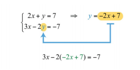.png?revision=1 "solving linear systems by elimination assignment")
This leaves you with an equivalent equation with one variable, which can be solved using the techniques learned up to this point.
Step 3 : Solve for the remaining variable. To solve for \(x\), first distribute \(−2\):
Step 4 : Back substitute to find the value of the other coordinate. Substitute \(x= 1\) into either of the original equations or their equivalents. Typically, we use the equivalent equation that we found when isolating a variable in step 1.
\(\begin{aligned} y&=-2x+7\\&=-2(\color{OliveGreen}{1}\color{black}{)+7}\\&=-2+7\\&=5 \end{aligned}\)
The solution to the system is \((1, 5)\). Be sure to present the solution as an ordered pair.
Step 5 : Check. Verify that these coordinates solve both equations of the original system:
\(\color{Cerulean}{Check:}\:\:\color{black}{(1,5)}\)
\(\begin{array}{c|c} {Equation\:1:}&{Equation\:2:}\\{2x+y=7}&{3x-2y=-7}\\{2(\color{OliveGreen}{1}\color{black}{)+(}\color{OliveGreen}{5}\color{black}{)=7}}&{3(\color{OliveGreen}{1}\color{black}{)-2(}\color{OliveGreen}{5}\color{black}{)=-7}}\\{2+5=7}&{3-10=-7}\\{7=7\quad\color{Cerulean}{\checkmark}}&{-7=-7\quad\color{Cerulean}{\checkmark}} \end{array}\)
The graph of this linear system follows:
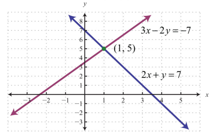.png?revision=1 "solving linear systems by elimination assignment")
The substitution method for solving systems is a completely algebraic method. Thus graphing the lines is not required.
Example \(\PageIndex{2}\)
\(\left\{\begin{aligned}2x−y&=1\\2x−y&=3\end{aligned}\right.\).
In this example, we can see that \(x\) has a coefficient of \(1\) in the second equation. This indicates that it can be isolated in one step as follows:
\(\begin{aligned} x-y&=3 \\ x-y\color{Cerulean}{+y}&=3\color{Cerulean}{+y} \\ x&=3+y \end{aligned}\)
\(\left\{\begin{aligned} 2\color{Cerulean}{x}\color{black}{-y}&=12 \\ x-y&=3 \Rightarrow \color{Cerulean}{x}\color{black}{=3+y} \end{aligned} \right.\)
Substitute \(3+y\) for \(x\) in the first equation. Use parentheses and take care to distribute.
\(\begin{aligned} 2x-y&=12\\2(\color{OliveGreen}{3+y}\color{black}{)-y}&=12 \\6+2y-y&=12 \\6+y&=12 \\ 6+y\color{Cerulean}{-6}&=12\color{Cerulean}{-6}\\y&=6 \end{aligned}\)
Use \(x=3+y\) to find \(x\).
\(\begin{aligned} x&=3+y\\&=3+\color{OliveGreen}{+6}\\&=9 \end{aligned}\)
\((9, 6)\). The check is left to the reader.
Example \(\PageIndex{3}\)
\(\left\{\begin{aligned}3x−5y&=1\\7x&=−1\end{aligned}\right.\).
In this example, the variable \(x\) is already isolated. Hence we can substitute \(x=−1\) into the first equation.
\((−1, −4)\). It is a good exercise to graph this particular system to compare the substitution method to the graphing method for solving systems.
Exercise \(\PageIndex{1}\)
\(\left\{\begin{aligned}3x+y&=4\\8x+2y&=10\end{aligned}\right.\).
Solving systems algebraically frequently requires work with fractions.
Example \(\PageIndex{4}\)
\(\left\{\begin{aligned}2x+8y&=5\\24x−4y&=−15\end{aligned}\right.\).
Begin by solving for \(x\) in the first equation.
\(\begin{aligned} 2x+8y&=5\\2x+8y\color{Cerulean}{-8y}&=5\color{Cerulean}{-8y} \\ \frac{2x}{\color{Cerulean}{2}}&=\frac{-8y+5}{\color{Cerulean}{2}} \\ x&=\frac{-8y}{2}+\frac{5}{2} \\ x&=-4y+\frac{5}{2} \end{aligned}\)
\(\left\{\begin{aligned} 2x+8y&=5 \Rightarrow \color{Cerulean}{x}\color{black}{=-4y+\frac{5}{2}} \\ 24\color{Cerulean}{x}\color{black}{-4y}&=-15\end{aligned}\right.\)
Next, substitute into the second equation and solve for \(y\).
Back substitute into the equation used in the substitution step:
\(\begin{aligned} x&=-4y+\frac{5}{2} \\ &=-4\left(\color{OliveGreen}{\frac{3}{4}} \right)\color{black}{+\frac{5}{2}} \\ &=-3+\frac{5}{2} \\ &=-\frac{6}{2} + \frac{5}{2} \\ &=-\frac{1}{2} \end{aligned}\)
\((-\frac{1}{2},\frac{3}{4})\)
As we know, not all linear systems have only one ordered pair solution. Recall that some systems have infinitely many ordered pair solutions and some do not have any solutions. Next, we explore what happens when using the substitution method to solve a dependent system.
Example \(\PageIndex{5}\)
\(\left\{\begin{aligned}−5x+y&=−1\\10x−2y&=2\end{aligned}\right.\).
Since the first equation has a term with coefficient \(1\), we choose to solve for that first.
Next, substitute this expression in for \(y\) in the second equation.
\(\begin{aligned} 10x-2y&=2 \\ 10x-2(\color{OliveGreen}{5x-1}\color{black}{)}&=2 \\ 10x-10x+2&=2 \\ 2&=2 \quad\color{Cerulean}{True} \end{aligned}\)
This process led to a true statement; hence the equation is an identity and any real number is a solution. This indicates that the system is dependent. The simultaneous solutions take the form \((x, mx + b)\), or in this case, \((x, 5x − 1)\), where \(x\) is any real number.
\((x, 5x−1)\)
To have a better understanding of the previous example, rewrite both equations in slope-intercept form and graph them on the same set of axes.
We can see that both equations represent the same line, and thus the system is dependent. Now explore what happens when solving an inconsistent system using the substitution method.
Example \(\PageIndex{6}\)
\(\left\{\begin{aligned}−7x+3y&=3\\14x−6y&=−16\end{aligned}\right.\).
Solve for \(y\) in the first equation.
\(\begin{aligned} -7x+3y&=3 \\ -7x+3y\color{Cerulean}{+7x}&=3\color{Cerulean}{+7x} \\3y&=7x+3 \\ \frac{3y}{\color{Cerulean}{3}}&=\frac{7x+3}{\color{Cerulean}{3}}\\y&=\frac{7}{3}x+1 \end{aligned}\)
\(\left\{\begin{aligned} -7x+3y&=3 \Rightarrow \color{Cerulean}{y}\color{black}{=\frac{7}{3}x+1} \\ 14x-6\color{Cerulean}{y}&=-16\end{aligned}\right.\)
Substitute into the second equation and solve.
Solving leads to a false statement. This indicates that the equation is a contradiction. There is no solution for \(x\) and hence no solution to the system.
No solution, \(Ø\)
A false statement indicates that the system is inconsistent, or in geometric terms, that the lines are parallel and do not intersect. To illustrate this, determine the slope-intercept form of each line and graph them on the same set of axes.
In slope-intercept form, it is easy to see that the two lines have the same slope but different \(y\)-intercepts.
Exercise \(\PageIndex{2}\)
\(\left\{\begin{aligned}2x−5y&=3\\4x−10y&=6\end{aligned}\right.\).
\((x, \frac{2}{5}x−\frac{3}{5}) \)
Key Takeaways
- The substitution method is a completely algebraic method for solving a system of equations.
- The substitution method requires that we solve for one of the variables and then substitute the result into the other equation. After performing the substitution step, the resulting equation has one variable and can be solved using the techniques learned up to this point.
- When the value of one of the variables is determined, go back and substitute it into one of the original equations, or their equivalent equations, to determine the corresponding value of the other variable.
- Solutions to systems of two linear equations with two variables, if they exist, are ordered pairs \((x, y)\).
- If the process of solving a system of equations leads to a false statement, then the system is inconsistent and there is no solution, \(Ø\).
- If the process of solving a system of equations leads to a true statement, then the system is dependent and there are infinitely many solutions that can be expressed using the form \((x, mx + b)\).
Exercise \(\PageIndex{3}\) Substitution Method
Solve by substitution.
- \(\left\{\begin{aligned} y&=4x−1\\−3x+y&=1\end{aligned}\right.\)
- \(\left\{\begin{aligned}y&=3x−8\\4x−y&=2 \end{aligned}\right.\)
- \(\left\{\begin{aligned}x&=2y−3\\x+3y&=−8 \end{aligned}\right.\)
- \(\left\{\begin{aligned}x&=−4y+12\\x+3y&=12 \end{aligned}\right.\)
- \(\left\{\begin{aligned}y&=3x−5\\x+2y&=2 \end{aligned}\right.\)
- \(\left\{\begin{aligned}y&=x\\2x+3y&=10 \end{aligned}\right.\)
- \(\left\{\begin{aligned}y&=4x+1\\−4x+y&=2 \end{aligned}\right.\)
- \(\left\{\begin{aligned}y&=−3x+5\\3x+y&=5 \end{aligned}\right.\)
- \(\left\{\begin{aligned}y&=2x+3\\2x−y&=−3 \end{aligned}\right.\)
- \(\left\{\begin{aligned}y&=5x−1\\x−2y&=5 \end{aligned}\right.\)
- \(\left\{\begin{aligned}y&=−7x+1\\3x−y&=4 \end{aligned}\right.\)
- \(\left\{\begin{aligned}x&=6y+2\\5x−2y&=0 \end{aligned}\right.\)
- \(\left\{\begin{aligned}y&=−2−2x\\−y&=−6 \end{aligned}\right.\)
- \(\left\{\begin{aligned}x&=−3x−4\\y&=−3 \end{aligned}\right.\)
- \(\left\{\begin{aligned}y&=−\frac{1}{5}x+\frac{3}{7}\\x−5y&=9 \end{aligned}\right.\)
- \(\left\{\begin{aligned}y&=\frac{2}{3}x−\frac{1}{6}\\x−9y&=0 \end{aligned}\right.\)
- \(\left\{\begin{aligned}y&=\frac{1}{2}x+\frac{1}{3}\\x−6y&=4 \end{aligned}\right.\)
- \(\left\{\begin{aligned}y&=−\frac{3}{8}x+\frac{1}{2}\\2x+4y&=1 \end{aligned}\right.\)
- \(\left\{\begin{aligned}x+y&=6\\2x+3y=\frac{1}{6} \end{aligned}\right.\)
- \(\left\{\begin{aligned}x−y&=3\\−2x+3y&=−2 \end{aligned}\right.\)
- \(\left\{\begin{aligned}2x+y&=2\\3x−2y&=\frac{1}{7} \end{aligned}\right.\)
- \(\left\{\begin{aligned}x−3y&=−\frac{1}{13}\\x+5y&=−5 \end{aligned}\right.\)
- \(\left\{\begin{aligned}x+2y&=−3\\3x−4y&=−2 \end{aligned}\right.\)
- \(\left\{\begin{aligned}5x−y&=12\\9x−y&=10 \end{aligned}\right.\)
- \(\left\{\begin{aligned}x+2y&=−6\\−4x−8y&=24 \end{aligned}\right.\)
- \(\left\{\begin{aligned}x+3y&=−6\\−2x−6y&=−12 \end{aligned}\right.\)
- \(\left\{\begin{aligned}−3x+y&=−4\\6x−2y&=−2 \end{aligned}\right.\)
- \(\left\{\begin{aligned}x−5y&=−10\\2x−10y&=−20 \end{aligned}\right.\)
- \(\left\{\begin{aligned}3x−y&=9\\4x+3y&=−1 \end{aligned}\right.\)
- \(\left\{\begin{aligned}2x−y&=5\\4x+2y&=−2 \end{aligned}\right.\)
- \(\left\{\begin{aligned}−x+4y&=0\\2x−5y&=−6 \end{aligned}\right.\)
- \(\left\{\begin{aligned}3y−x&=5\\5x+2y&=−8 \end{aligned}\right.\)
- \(\left\{\begin{aligned}2x−5y&=1\\4x+10y&=2 \end{aligned}\right.\)
- \(\left\{\begin{aligned}3x−7y&=−3\\6x+14y&=0 \end{aligned}\right.\)
- \(\left\{\begin{aligned}10x−y&=3\\−5x+12y&=1 \end{aligned}\right.\)
- \(\left\{\begin{aligned}−\frac{1}{3}x+\frac{1}{6}y&=\frac{2}{3}\\ \frac{1}{2}x−\frac{1}{3}y&=−\frac{3}{2} \end{aligned}\right.\)
- \(\left\{\begin{aligned}\frac{1}{3}x+\frac{2}{3}y&=1 \\ \frac{1}{4}x−\frac{1}{3}y&=−\frac{1}{12} \end{aligned}\right.\)
- \(\left\{\begin{aligned}\frac{1}{7}x−y&=\frac{1}{2}\\ \frac{1}{4}x+\frac{1}{2}y&=2 \end{aligned}\right.\)
- \(\left\{\begin{aligned}−\frac{3}{5}x+\frac{2}{5}y&=\frac{1}{2}\\ \frac{1}{3}x−\frac{1}{12}y&=−\frac{1}{3} \end{aligned}\right.\)
- \(\left\{\begin{aligned}\frac{1}{2}x&=\frac{2}{3}y\\x−\frac{2}{3}y&=2 \end{aligned}\right.\)
- \(\left\{\begin{aligned}−\frac{1}{2}x+\frac{1}{2}y&=\frac{5}{8} \\ \frac{1}{4}x+\frac{1}{2}y&=\frac{1}{4} \end{aligned}\right.\)
- \(\left\{\begin{aligned}x−y&=0\\−x+2y&=3 \end{aligned}\right.\)
- \(\left\{\begin{aligned}y&=3x\\2x−3y&=0 \end{aligned}\right.\)
- \(\left\{\begin{aligned}2x+3y&=18\\−6x+3y&=−6 \end{aligned}\right.\)
- \(\left\{\begin{aligned}−3x+4y&=20\\ 2x+8y&=8 \end{aligned}\right.\)
- \(\left\{\begin{aligned}5x−3y&=−1\\ 3x+2y&=7 \end{aligned}\right.\)
- \(\left\{\begin{aligned}−3x+7y&=2\\ 2x+7y&=1 \end{aligned}\right.\)
- \(\left\{\begin{aligned}y&=3\\y&=−3 \end{aligned}\right.\)
- \(\left\{\begin{aligned}x&=5\\x&=−2 \end{aligned}\right.\)
- \(\left\{\begin{aligned}y&=4\\y&=4\end{aligned}\right.\)
1. \((2, 7)\)
3. \((−5, −1)\)
5. \((2, 6)\)
7. \(∅\)
9. \((x, 2x+3)\)
11. \((\frac{1}{2}, −\frac{5}{2})\)
13. \((4, −2)\)
15. \((3, \frac{12}{5})\)
17. \((−3, −\frac{7}{6})\)
19. \((2, 4)\)
21. \((3, −4)\)
23. \((−\frac{8}{5}, −\frac{7}{10})\)
25. \((x, −\frac{1}{2}x−3)\)
27. \(∅\)
29. \((2, −3)\)
31. \((−8, −2)\)
33. \((\frac{1}{2}, 0)\)
35. \(∅\)
37. \((1, 1)\)
39. \((−\frac{11}{10}, −\frac{2}{5})\)
41. \((−\frac{1}{2}, \frac{3}{4})\)
43. \((0, 0)\)
45. \((−4, 2)\)
47. \((−\frac{1}{5}, \frac{1}{5})\)
49. \(∅\)
Exercise \(\PageIndex{4}\) Substitution Method
Set up a linear system and solve it using the substitution method.
- The sum of two numbers is \(19\). The larger number is \(1\) less than three times the smaller.
- The sum of two numbers is \(15\). The larger is \(3\) more than twice the smaller.
- The difference of two numbers is \(7\) and their sum is \(1\).
- The difference of two numbers is \(3\) and their sum is \(−7\).
- Where on the graph of \(−5x+3y=30\) does the \(x\)-coordinate equal the \(y\)-coordinate?
- Where on the graph of \(\frac{1}{2}x−\frac{1}{3}y=1\) does the \(x\)-coordinate equal the \(y\)-coordinate?
1. The two numbers are \(5\) and \(14\).
3. The two numbers are \(4\) and \(−3\).
5. \((−\frac{1}{5}, −\frac{1}{5})\)
Exercise \(\PageIndex{5}\) Discussion Board Topics
- Describe what drives the choice of variable to solve for when beginning the process of solving by substitution.
- Discuss the merits and drawbacks of the substitution method.
1. Answers may vary
IMAGES
VIDEO
COMMENTS
1/12. 1/8. 6x - 2y = 28x + 3y = 14Explain how knowing how to find the least common multiple (LCM) of two numbers can help you solve the system of equations presented here by eliminating the x-terms. The LCM of 6 and 8 is 24. Knowing this, multiply the first equation by 4 and the second by −3 to get opposite coefficients.
Example 1. We're asked to solve this system of equations: 2 y + 7 x = − 5 5 y − 7 x = 12. We notice that the first equation has a 7 x term and the second equation has a − 7 x term. These terms will cancel if we add the equations together—that is, we'll eliminate the x terms: 2 y + 7 x = − 5 + 5 y − 7 x = 12 7 y + 0 = 7.
Infinite number of solutions. 23) −14 =. 24) (2, 0) (−1, 1) Create your own worksheets like this one with Infinite Algebra 1. Free trial available at KutaSoftware.com. ©q R2h041222 cK7uitqaL ASPovfPthwEanrQed vLOLrCy.6 w AAVlXl9 wrxivgghCtUsC xrmeAsfeGrivpe9du.Q Q iMwaHdMeB GwSijtZht xIrnOfNiRnFiotLeH 1AAlSgheWb4r0aG X1K.J.
Elimination Method. Elimination Method (Systems of Linear Equations) The main concept behind the elimination methodis to create terms with opposite coefficientsbecause they cancel each other when added. In the end, we should deal with a simple linear equation to solve, like a one-step equation in [latex]x[/latex] or in [latex]y[/latex].
Systems of equations: trolls, tolls (2 of 2) Testing a solution to a system of equations. Systems of equations with graphing: y=7/5x-5 & y=3/5x-1. Systems of equations with graphing: exact & approximate solutions. Setting up a system of equations from context example (pet weights) Setting up a system of linear equations example (weight and price)
Elimination method review (systems of linear equations) Equivalent systems of equations review. Math > Algebra (all content) > System of equations > ... Let's explore a few more methods for solving systems of equations. Let's say I have the equation, 3x plus 4y is equal to 2.5. And I have another equation, 5x minus 4y is equal to 25.5.
Learn how to solve linear systems by elimination, a method that involves adding or subtracting equations to eliminate one variable and find the solution. This book chapter from Mathematics LibreTexts explains the steps and examples of using the elimination method in different cases.
Section 5.3 Solving Systems of Linear Equations by Elimination 213 EXAMPLE 2 Solving a System of Linear Equations by Elimination Solve the system by elimination. −6x + 5y = 25 Equation 1 −2x − 4y = 14 Equation 2 Step 1: Notice that no pairs of like terms have the same or opposite coeffi cients. One way to solve by elimination is to multiply Equation 2 by 3 so that the x-terms have a ...
This lesson focuses on solving systems of linear equations using elimination. See different methods for solving equations using elimination through several examples. Click Create Assignment to assign this modality to your LMS.
Solve the system of equations. To solve the system of equations, use elimination. The equations are in standard form and the coefficients of m are opposites. Add. {n + m = 39 n − m = 9 _ 2n = 48 Solve for n. n = 24 Substitute n=24 into one of the original n + m = 39 equations and solve form. 24 + m = 39 m = 15 Step 6.
Introduction; 2.1 Solve Equations Using the Subtraction and Addition Properties of Equality; 2.2 Solve Equations using the Division and Multiplication Properties of Equality; 2.3 Solve Equations with Variables and Constants on Both Sides; 2.4 Use a General Strategy to Solve Linear Equations; 2.5 Solve Equations with Fractions or Decimals; 2.6 Solve a Formula for a Specific Variable
4.3: Solving Systems by Elimination. Page ID. David Arnold. College of the Redwoods. When both equations of a system are in standard form \ (Ax + By = C\), then a process called elimination is usually the best procedure to use to find the solution of the system. Elimination is based on two simple ideas, the first of which should be familiar.
What is the Elimination Method? It is one way to solve a system of equations. The basic idea is if you have 2 equations, you can sometimes do a single operation and then add the 2 equations in a way that eleiminates 1 of the 2 variables as the example that follows shows.
Step 1. Eliminate one variable to obtain a linear system in two variables. Step 2. Solve the new linear system for both of its variables. Step 3. Substitute the values found in Step 2 into one of the original equations. and solve for the remaining variable. When you obtain a false equation, such as 0.
Let's solve a few more systems of equations using elimination, but in these it won't be kind of a one-step elimination. We're going to have to massage the equations a little bit in order to prepare them for elimination. So let's say that we have an equation, 5x minus 10y is equal to 15. And we have another equation, 3x minus 2y is equal to 3.
Use this lesson to introduce students to the elimination method for solving systems of equations. Students will learn that adding multiples of the original equations produces a new equation of a line that has the same intersection point as the original equations. This visual introduction helps students self-check their algebraic steps along the way.
Free lessons, worksheets, and video tutorials for students and teachers. Topics in this unit include: solving linear systems by graphing, substitution, elimination, and solving application questions. This follows chapter 1 of the principles of math grade 10 McGraw Hill textbook.
Section 8.3 Solving Systems by Elimination. A1.3.12 Represent and solve problems that can be modeled using a system of linear equations and/or inequalities in two variables, sketch the solution sets, and interpret the results within the context of the problem;
4.3: Solving Linear Systems by Elimination; 4.4: Applications of Linear Systems; 4.5: Solving Systems of Linear Inequalities (Two Variables) A system of linear inequalities consists of a set of two or more linear inequalities with the same variables. The inequalities define the conditions that are to be considered simultaneously.
Solving linear equations using Gaussian elimination and back substitution (Str§1.3). Cost (number of operations, Str§1.3). ... to solve the corresponding linear system of equations.This may be alleviated by some degree using complete (full) pivoting. ... and then point assignment to cluster the rest of the data) (l)Outlier/ anomaly detection ...
Use Gaussian elimination to solve the given 2 × 2 2 × 2 system of equations. 2x + y 4x + 2y = 1 = 6 2 x + y = 1 4 x + 2 y = 6. Solution. Write the system as an augmented matrix. [ 2 4 1 2 1 6] [ 2 1 1 4 2 6] Obtain a 1 1 in row 1, column 1. This can be accomplished by multiplying the first row by 1 2 1 2.
Solve by substitution: Solution: Step 1: Solve for either variable in either equation. If you choose the first equation, you can isolate y in one step. 2x + y = 7 2x + y− 2x = 7− 2x y = − 2x + 7. Step 2: Substitute the expression − 2x + 7 for the y variable in the other equation. Figure 4.2.1.