short case study on drought in india

Accessibility Links

• Skip to content
• Skip to search IOPscience
• Skip to Journals list
• Accessibility help
• Accessibility Help

Click here to close this panel.

Purpose-led Publishing is a coalition of three not-for-profit publishers in the field of physical sciences: AIP Publishing, the American Physical Society and IOP Publishing.

Together, as publishers that will always put purpose above profit, we have defined a set of industry standards that underpin high-quality, ethical scholarly communications.

We are proudly declaring that science is our only shareholder.

Unprecedented drought in South India and recent water scarcity

Vimal Mishra 4,1,2 , Kaustubh Thirumalai 3 , Sahil Jain 1 and Saran Aadhar 1

Published 16 April 2021 • © 2021 The Author(s). Published by IOP Publishing Ltd Environmental Research Letters , Volume 16 , Number 5 Citation Vimal Mishra et al 2021 Environ. Res. Lett. 16 054007 DOI 10.1088/1748-9326/abf289

You need an eReader or compatible software to experience the benefits of the ePub3 file format .

Article metrics

8430 Total downloads

Share this article

Author e-mails.

[email protected]

Author affiliations

1 Civil Engineering, Indian Institute of Technology (IIT) Gandhinagar, Gandhinagar, Gujarat 382355, India

2 Earth Sciences, Indian Institute of Technology (IIT) Gandhinagar, Gandhinagar, Gujarat 382355, India

3 Department of Geosciences, University of Arizona, 1040 E. 4th Street, Tucson, AZ 85721, United States of America

Author notes

4 Author to whom any correspondence should be addressed.

Vimal Mishra https://orcid.org/0000-0002-3046-6296

Kaustubh Thirumalai https://orcid.org/0000-0002-7875-4182

Saran Aadhar https://orcid.org/0000-0003-1645-4093

• Received 25 November 2020
• Accepted 26 March 2021
• Published 16 April 2021

Peer review information

Method : Single-anonymous Revisions: 1 Screened for originality? Yes

Buy this article in print

Peninsular Indian agriculture and drinking water availability are critically reliant on seasonal winter rainfall occurring from October to December, associated with the northeastern monsoon (NEM). Over 2016–2018, moderate-to-exceptionally low NEM rainfall gave rise to severe drought conditions over much of southern India and exacerbated water scarcity. The magnitude and dynamics of this drought remain unexplored. Here, we quantify the severity of this event and explore causal mechanisms of drought conditions over South India. Our findings indicate that the 3-year cumulative rainfall totals of NEM rainfall during this event faced a deficit of more than 40%—the driest 3-year period in ∼150 years according to the observational record. We demonstrate that drought conditions linked to the NEM across South India are associated with cool phases in the equatorial Indian and Pacific Oceans. Future changes in these teleconnections will add to the challenges of drought prediction.

Export citation and abstract BibTeX RIS

Original content from this work may be used under the terms of the Creative Commons Attribution 4.0 license . Any further distribution of this work must maintain attribution to the author(s) and the title of the work, journal citation and DOI.

1. Introduction

Deficiency of the summer monsoonal precipitation is one of the main drivers of meteorological drought in India, which if prolonged, can transform into more impactful agricultural and hydrological droughts (Mishra and Singh 2010 , Mishra et al 2010 , Mo 2011 ). Agricultural and hydrological droughts can pose lasting impacts on food production and water availability, respectively (Van Loon 2015 , Samaniego et al 2018 , Mishra 2020 ). India experiences two major monsoon seasons—the Indian summer monsoon (ISM), also known as the southwestern monsoon and the lesser-studied northeastern monsoon (NEM) or the winter monsoon (Gadgil and Gadgil 2006 , Rajeevan et al 2012 ). The ISM is the major source of precipitation for much of India over the period of June to September (hereafter JJAS) and has been the focus of extensive study (Gadgil and Gadgil 2006 , Singh et al 2019 ). On the other hand, the NEM is more important in selected parts of India and is associated with rainfall during the period between October and December (hereafter OND) (Kripalani and Kumar 2004 , Zubair and Ropelewski 2006 , Yadav 2012 ). In particular, the NEM significantly impacts peninsular India, where certain parts of South India receive a majority of their annual rainfall totals during the OND season (Rajeevan et al 2012 ). Despite lesser precipitation totals compared to the ISM, the NEM is critically important for water availability, agriculture, and the livelihood of millions of people residing in peninsular India.

Previously, studies have indicated that both monsoon seasons have experienced profound changes over the past few decades (Mishra et al 2012 , Rajeevan et al 2012 , Roxy et al 2015 , Singh et al 2019 ). For instance, seasonal mean precipitation associated with the ISM has shown a declining trend leading to more frequent monsoon-season deficits (Mishra et al 2012 , Christensen et al 2013 , Roxy et al 2015 ). Similarly, the increase in precipitation associated with the NEM over the last few decades has been attributed to the warming of the Indian Ocean (Mishra et al 2012 , Roxy et al 2015 ). Furthermore, the El Niño Southern Oscillation (ENSO) and Indian Ocean Dipole (IOD) phenomena are well-known drivers of deficits in monsoon rainfall (Ashok et al 2001 , Kumar et al 2007 ) and are also expected to undergo changes with ongoing increases in greenhouse gases (Cai et al 2018 , Timmermann et al 2018 ). Addressing the mechanisms of why and how these monsoon seasons are shifting under a warming world is critical for improving predictions of drought conditions in India.

Whereas previous studies have shown strong linkages between summer monsoon droughts in India and sea surface temperature (SST) variability in the equatorial Indian and Pacific Oceans (Kripalani and Kulkarni 1997 , Barlow et al 2002 , Niranjan Kumar et al 2013 , Roxy et al 2015 ), few studies have focused on the causes of rainfall deficits associated with the NEM (Dimri et al 2016 ). From 2016 to 2018, South India witnessed severe drought conditions, which significantly impacted agriculture and water availability in the region ('Chennai water crisis: City's reservoirs run dry,' BBC 2019 ). The densely populated states of Andhra Pradesh, Karnataka, and Tamil Nadu continuously declared drought in 2016, 2017, and 2018 related to the deficits in NEM precipitation. The drought caused water crises in both urban and rural areas (Aguilera 2019 ). Despite the profound impacts of the 2016–18 drought in South India, its magnitude, drivers, and mechanisms remain unexplored. In this study, we focus on the 2016–2018 drought, quantify its severity, and investigate its causes and relationships with regional and global ocean–atmosphere variability. We place this extreme event in the context of the previous droughts and conclude that its severity was unprecedented over the observational record.

2. Data and methods

The NEM (October–December) is a dominant source of rainfall in South India (Rajeevan et al 2012 ). South India (Latitude: 8°N–15°N; Longitude: 74°E–81°E)) comprises of five Indian states and three union territories. The region encompasses nearly 19% of India's area and harbors around 250 million people, which is one-fifth of the total population of India (Census of India 2011 ). South India is an agriculturally rich part of the country, with over 60% of its rural population engaged in agriculture (Aulong et al 2012 ). The population depends largely on the NEM for agricultural production. We used gridded daily precipitation data available at 0.5° spatial resolution for the period of 1870–2018 (Mishra et al 2019 ). Mishra et al ( 2019 ) used station observations from India Meteorology Department (IMD) to develop the gridded precipitation for the pre-1900 (1870–1900) period, which was merged with the gridded data available for the post-1900 period (1901–2018; (Pai et al 2014 )) from IMD. More details on the gridded precipitation data and evaluation of its quality can be obtained from Mishra et al ( 2019 ). The gridded data capture orographic precipitation along the Western Ghats, Northeast, and the foothills of Himalaya (Pai et al 2014 , Mishra et al 2019 ).

Total water storage (TWS) data were obtained from the Gravity Recovery and Climate Experiment (GRACE) and GRACE follow on (GRACE-FO) missions. TWS is available for the period April 2002 to June 2017 from the GRACE satellites. The GRACE-FO mission provides the data from June 2018 to present. Therefore, the TWS data for July 2017 to May 2018 is not available. We obtained TWS from GRACE and GRACE-FO from NASA's Jet Propulsion Lab (JPL: https://podaac.jpl.nasa.gov/dataset/TELLUS_GRAC-GRFO_MASCON_CRI_GRID_RL06_V2 ) for the 2002–2019 period. The GRACE mascon product (RL06 V2) contains gridded monthly global water storage anomalies relative to mean, which is available at 0.5° spatial resolution (Wiese et al 2016 ). To remove the seasonal cycle from TWS, monthly mean TWS was removed from each month, and scale factors were applied.

To assess the influence of SSTs on the 2016–18 drought, we used monthly data from the HadSST dataset (Hadley Centre) for the period 1870–2018 at 2.0° spatial resolution (Rayner et al 2003 ). We obtained surface air temperatures (SATs) from Berkley Earth (Rohde et al 2013 ) to analyze anomalous temperature conditions during NEM droughts. Since SST data has a strong warming trend, we used Ensemble Empirical Mode Decomposition (EEMD; (Wu and Huang 2009 )) to remove the secular trend (Wu et al 2011 ) from SST time series as in Mishra ( 2020 ). The EEMD method has an advantage over conventional detrending as it removes both linear and non-linear trends (Mishra 2020 ). We estimated SST and precipitation anomalies for the NEM (October–December) to diagnose the linkage between precipitation and SST. To examine the coupled variability of precipitation and SST, we use maximum covariance analysis (MCA; (Bretherton et al 1992 )). In addition, we used empirical orthogonal function (EOF) analysis to obtain the dominant modes of variability in rainfall during the NEM when SST was not used. The MCA, performed on two fields (here precipitation and SST) together, identifies the leading modes of variability in which the variations of the two fields are strongly coupled (Mishra et al 2012 ). Sea level pressure (SLP) and wind fields (horizontal, u and meridional, v) were obtained from the European Centre for Medium-Range Weather Forecasts Reanalysis version 5 (ERA-5; (Hersbach and Dee 2016 )) for the period 1979–2018 to understand the mechanism of the northeast monsoon. Further, SLP and wind fields were regridded to 2° to make them consistent with SST.

Towards predictability of NEM rainfall, we employed univariate and multivariate techniques. We use the lagged relationship between SST anomalies and rainfall over South Asia during the NEM as a predictor of OND rainfall. We used SST anomalies from the Nino 3.4 region and over the northern Indian Ocean (NIO; 6°–24°N, 40°–100°E) as a predictor of monthly NEM precipitation using the following three equations:

3.1. Unprecedented recent failure of northeast monsoon rainfall

South India receives more than 40% of its total annual precipitation during the NEM season (figure S1 (available online at stacks.iop.org/ERL/16/054007/mmedia )), and thus deficits in NEM rainfall pose significant water-related challenges in the region. To investigate the long-term observational history of NEM rainfall in the region, we used rainfall observations from the IMD (Pai et al 2014 ), spanning from 1870 to 2018. Domain-averaged precipitation anomalies associated with the NEM indicate that most of South India experienced exceptional (>40%) precipitation deficits during 1874–1876 and 2016–2018 (figure 1 ). We calculated precipitation anomalies during the NEM for one, two, and three consecutive year durations over the 1870–2018 period to estimate abnormal deficit-years in the long-term record (figures 1 , 2 and S4, table 1 ). There are five pronounced periods of drought (>29% deficits) in the overall record including the recent drought of 2016–2018, the droughts during 2001–03, 1949–1951, 2002–04, and the well-known Great Drought of 1876–78 (Cook et al 2010 , Singh et al 2018 ), which was associated with the Great Madras Famine (Blanford 1884 , Mishra et al 2019 ). Among these events, our analysis indicates that the Great Drought and the recent event of 2016–18 are the most severe (figure 1 ). During 2016–18, South India experienced the worst NEM drought over the last 150 years with a precipitation deficit of 45%, whereas the 1874–76 drought was the second-worst, with a deficit of 37% (table 1 ). We note that the 1-year and 2-year duration NEM deficits for 1876 (69%) and 1876–77 (54%) were comparable to the deficits during 2016 (63%) and the 2016–17 (52%) durations (table 1 , figures S2–S4). However, the consecutive 3-year NEM deficit for 2016–18 was more significant than the Great Drought. We find that annual rainfall anomalies additionally indicate drought conditions in 2016, 2017, and 2018 (figure S5). Moreover, 2 and 3-year annual rainfall anomalies for 2016–17 and 2016–18 also show a major rainfall deficit in South India (figure S5). Thus, we conclude that the 2016–18 drought caused by the failure of the NEM also contained severe annual rainfall deficits.

Figure 1.  Three-year cumulative precipitation anomalies (mm) during the Northeast monsoon (NEM, October–December). (a), (b) The spatial pattern of 3 year cumulative precipitation anomalies (mm) during 1874–1876 and 2016–2018 periods, respectively, in southern India (denoted by the green box). (c) Area-averaged (over the green box) 3 year moving-mean precipitation anomalies (%) for the period 1870–2016. Red dots in (c) demarcate the two periods of interest, and show that the 2016–18 was the 1st and 1874–76 was the 2nd worst drought in last 150 years. Long-term precipitation data is based on station observations from the Indian Meteorological Department (IMD).

Download figure:

Figure 2.  Total water storage (TWS) anomalies from the GRACE and GRACE–FO during 2002–2019. (a)–(c) TWS anomalies (cm) during December 2016, June 2017, and June 2019. (d) 12-month moving-sum precipitation anomalies (cm, in blue) and monthly TWS anomalies (cm, in red) aggregated over South India (south of 15°N). Note that the July 2017 to May 2018 period contains missing data as the GRACE-FO dataset is only available from June 2018 onwards. The Pearson correlation coefficient between TWS anomalies and precipitation anomalies is 0.63.

Table 1.  Top five driest years for one, two, and three-year cumulative northeast monsoon (OND).

Over individual NEM seasons, the two most extreme dry events occurred in 1876 and 2016 with precipitation deficits of 69% and 63%, respectively (table 1 ). The rainfall deficit in 2016 was more severe in comparison to the lack of precipitation in 2017 and 2018 (figure S2). The failure of the NEM in 2016 as well as relatively low rainfall totals over the consecutive years were the main causes behind the 2016–18 drought in South India (table 1 ). Overall, the 3-year NEM drought of 2016–2018 was more severe than the Great Drought of 1874–1876. Infamously, the 1876 drought resulted in famine and the deaths of millions of people (Mishra et al 2019 , Mishra 2020 ). The more recent 2016–18 NEM drought considerably influenced water availability in the region and caused a water crisis across South India ('Chennai water crisis: City's reservoirs run dry,' BBC 2019 ).

Furthermore, the 2016–2018 NEM drought in South India was unprecedented in the last 150 years and had severe implications for water availability. TWS from the GRACE and GRACE–FO satellites showed a considerable loss in South India due to the recent (2016–2018) drought (figure 2 ). Twelve months moving precipitation anomalies pinpoint the onset of drought in South India during October 2016 and show that it continued till October 2018 (figure 2 ). Although there was a weak recovery from drought conditions for two months in November and December 2018, these rainfall totals were not enough to negate the influence of the overall event (2016–2018), which continued till August 2019 (figure 2 ), and was only alleviated by stronger NEM rains later that year. We also note that 12-month precipitation anomalies and TWS anomalies are well-correlated ( r = 0.63), where local observations indicate that rainfall is the major contributor of TWS (Asoka et al 2017 ). Thus, we attribute the loss in regional TWS to the long-term 3-year drought, which was precipitated by the lack of NEM rainfall.

Total water loss in South India estimated from the GRACE satellite was 79 km 3 in December 2016 (figure 2 (a)). Similarly, GRACE–FO data reveal that total water loss in June 2017 and 2019 was 46.5 and 41.7 km 3 , respectively (figures 2 (b) and (c)). Recovery in TWS occurred in late 2019 due to improved NEM rainfall over the region. The 2016–2018 drought caused a significant loss in TWS, which also likely resulted in a significant depletion in groundwater across South India. We caveat that we did not estimate the overall loss in groundwater due to uncertainty in soil moisture (Long et al 2013 , Castle et al 2014 )—an estimate outside the scope of this work—however we suspect that the groundwater depletion was driven by the drought in addition to increased groundwater extraction (Thomas et al 2017 ) during the drought (Asoka et al 2017 ). Despite the uncertainty in the estimation of total water loss from GRACE satellites (Long et al 2013 ), the combined influence of depletion in surface-water and groundwater during this event led to unprecedented water scarcity in South India (Aguilera 2019 , 'Chennai water crisis: City's reservoirs run dry,' BBC 2019 ).

3.2. Mechanism of deficit during the Northeast monsoon

We examined circulation patterns to understand mechanisms behind variability in NEM rainfall. To do so, we first examined climatological surface temperatures (SAT and SST), sea-level pressure (SLP), and wind fields at 850 hPa during the OND season (figure 3 ). SLP and wind fields were taken from the ERA-5 reanalysis dataset (Hersbach and Dee 2016 ) whereas SSTs and SATs were taken from HadSST (Rayner et al 2003 ) and Berkley Earth (Rohde et al 2013 ), respectively. Climatologically during boreal fall, cooling SATs over the northwestern Pacific and northern latitudes alongside comparatively warmer mean-annual SSTs over the northern Indian Oceans set up easterly wind flow across the Bay of Bengal (figures 3 (a) and (b)). In particular, warm SSTs in the western Indian Ocean can elicit easterlies across the Indian Ocean and favor moisture transport from the Bay of Bengal into peninsular India. These moisture-bearing winds, which become northeasterly before landfall, bring NEM rainfall to South India (Rajeevan et al 2012 ). Strong winds from across the South China Sea, driven by the underlying SAT and SLP patterns ultimately facilitate NEM rainfall. Thus, El-Niño-like conditions in the Pacific with cooler SSTs in the northern portion of the western tropical Pacific Ocean, juxtaposed with cooler SSTs in the eastern Indian Ocean and warmer SSTs in the west (i.e. resembling positive IOD-like conditions), all serve to enhance NEM rainfall over South India. It is to be expected that circulation patterns which weaken these processes ought to yield diminished NEM rainfall.

Figure 3.  Atmospheric and oceanic patterns during the 2016–18 drought in South India. (a), (b) Climatological mean surface-air temperature (SAT, °C) and sea-surface temperature (SST, °C), mean sea-level pressure (SLP, Pa) and wind at 850 hPa (in (b)) during the October–December (OND) season. (c), (d) SST, SLP, and wind anomalies associated with the NEM during the OND season of 2016, (e), (f) 2017, and (g), (h) 2018. Mean SLP and wind fields were obtained from ERA-5 whereas SST was taken from HadSST and SAT from BEST.

To better understand the causes of rainfall deficits, we investigated anomalous patterns during the NEM season for 2016, 2017, and 2018 (figure 3 ). In 2016 and 2017, as expected, cool SST anomalies prevailed in the tropical Indo-Pacific and were associated with La Niña conditions in the central Pacific along with negative IOD-like conditions in the Indian Ocean (figures 3 (c)–(f)). Both years witnessed anomalously cooler SSTs in the eastern tropical Indian Ocean and western tropical Pacific, and warmer SSTs in the western Indian Ocean and central Pacific. These SST patterns, alongside SLP and adjacent continental SAT patterns, gave rise to anomalous westerlies in the equatorial Indian Ocean, which weakened moisture transport from the Bay of Bengal during the NEM season of both events (figures 3 (c)–(f)). Moreover, both years were associated with anomalously low SLP and cooler surface temperatures across the Indian sub-continent and Bay of Bengal, sustaining an anomalous anticyclonic pattern which inhibited moisture transport into South India (figures 3 (c)–(f)). In 2018, the rainfall deficit conditions were slightly alleviated due to favorable warm conditions in the western tropical Indian Ocean and cooling in the East (development of a positive IOD event) alongside the development of El-Niño-conditions in the Pacific. However, it should be noted that western Indian Ocean warming was not particularly pronounced that year and alongside cooler temperature anomalies in the northern Indian Ocean, resulted in an overall deficit in NEM rainfall that year.

Next, we analyzed surface temperature and precipitation anomalies for the five most severe dry events in South India over the 1870–2018 period during the NEM season (figure 4 ). The major droughts in South India occurred in 1876, 2016, 1938, 1988, and 1974 (in order of severity). Out of these five droughts, four occurred during La Niña conditions. In contrast, the well-studied drought of 1876 during the NEM was linked with El Niño (figure 4 )—a finding reported previously (Cook et al 2010 , Singh et al 2018 , Mishra et al 2019 ). However, it should be noted that cool SST conditions prevailed in the Pacific Ocean over the 1870–1876 period and the transition from the cool to warm phase occurred during the NEM season of 1876 (Singh et al 2018 ). Additionally, the western Indian Ocean was not anomalously warm as it typically is during El Niño years (figure 4 (a)). Nevertheless, temperature and SLP anomaly composites for the most severe dry and wet NEM years reveal a general propensity for cooler SSTs in the Indo–Pacific (i.e. La Niña conditions) to be associated with precipitation deficits over South India (figures S6 and S7). On the other hand, warming in the central Pacific and Indian Oceans is associated with a stronger NEM and surplus precipitation (figure S7). Overall, OND cooling in the Indian and central Pacific oceans results in lower SLP and weaker wind fields, which ultimately drive rainfall deficits in South India.

Figure 4.  Sea surface temperature (SST)/surface air temperature (SAT) and precipitation (P) anomalies for the top five droughts that occurred in South India during the northeast monsoon for 1870–2018 period. SST and SAT datasets were obtained from Hadley Center and Berkley Earth, respectively. SAT data over few regions are not available for 1876.

3.3. SST variability during Northeast Monsoon

To clarify the relationship between SST and precipitation anomalies associated with the NEM, we performed MCA, which helps delineate the leading patterns responsible for co-variability between South Indian NEM rainfall and tropical SSTs. The first leading mode exhibits typical ENSO-like patterns of covariance and explains 77.2% of total variance (figure 5 (a)). As demonstrated above with patterns of the major droughts (figure 4 ), MCA also indicates that negative SST anomalies over the central Pacific (i.e. La Niña) and Indian Oceans (negative IOD) result in below normal NEM precipitation over South India (figure 5 (b)). The second leading mode of MCA exhibits a relatively weaker relationship between precipitation and SST anomalies during the NEM (figure 5 ). The second mode fingerprints the role of SST warming in the Indian Ocean as a driver of increased NEM precipitation in South India (Roxy et al 2015 ). We also note that there appears to be a slight dichotomy between northern and southern South India, where NEM precipitation in the latter region is more strongly linked with ENSO (figure 5 ). On the other hand, precipitation over the northern parts of South India is more strongly associated with the second leading mode (figure 5 ). This finding might help explain some of the ambiguity surrounding the mechanisms of the impact of the 1876–78 Great Drought on South Indian rainfall. Overall, the leading mode of SST and precipitation variability during the NEM shows that cold SST anomalies in the Indo-Pacific facilitate drought conditions over South India.

Figure 5.  Links between South Indian precipitation and sea surface temperature (SST) during the Northeastern Monsoon season. (a), (b) Correlation patterns obtained from the first leading mode of maximum covariance analysis (MCA) performed between precipitation across South India (8°N–15°N and 74°E–81°E; see Green Box in figure 1 ) and SST during the October–November–December (OND) season over 1870–2018. (c), (d) Same as in the above panels but for the second leading mode of MCA. Rainfall was obtained from the IMD dataset whereas SST was retrieved from HadSST.

We performed EOF analysis to identify the dominant patterns of NEM rainfall in South India (figure 6 ). The first leading mode from the EOF analysis picks out rainfall variability across the entirety of South India and explains 50% of total variance (figure 6 (a)). The second leading mode reveals a bipolar rainfall pattern across the northern and southern parts of South India and explains 11% of the total variance (figure 6 ). We note that the characteristics of rainfall variability derived from the first and second modes of EOF analysis are consistent with the leading modes obtained from the MCA (figure 5 ). Taken together, our findings inferred from both EOFs and MCA show that the first leading mode affects rainfall across South India, whereas the second leading mode delineates opposing rainfall trends in the North versus the southern parts of South India (figure 6 ).

Figure 6.  The leading modes obtained from the empirical orthogonal function (EOF) analysis of rainfall during the NEM for the 1870–2018 period. (a) The first leading EOF mode of NEM, which explains 50.6% of the total variance in NEM rainfall in South India. (b) Lagged correlation between the first leading principle component (PC 1) and 3-month mean SST anomalies over different regions (Nino 3.4 (5°S–5°N, 120–170°W), North Indian Ocean (NIO; 6°–24°N, 40–100°E), North Pacific Ocean (NPO; 30°N–50°N, 120°E–175°W), North Atlantic Ocean (NAO; 6°–24°N, 10–60°W), Pacific Decadal Oscillation (PDO), and Southern Oscillation Index (SOI)). (c) and (d) same as (a) and (b) but for the second leading EOF mode and the corresponding PC 2. Year − 1, Year + 0, and Year + 1 represent the previous, current, and next year of the NEM season, respectively.

We calculated principal components (PCs) associated with the leading modes of variability derived from the EOF analysis (PC1 and PC2) to examine the predictability of NEM rainfall using SST anomalies (figure S8). We also computed the correlation between PC1 and SST anomalies in addition to oceanic indices (table S1) at different time lags (tables S2 and S3). We find that the first principal component (PC1) is strongly correlated ( r = 0.23, P -value < 0.05) to SSTs from April–June (AMJ) in the Nino 3.4 region (figure 6 ). However, PC2 is more appropriately delineated by ( r = 0.33, P -value < 0.05) SST anomalies from OND in Nino 3.4 and in the NIO (figure 6 ). We use this lagged relationship between oceanic indices and SST anomalies with PCs to establish a predictive model for NEM rainfall (as in Zhou et al 2019 ). Focusing on the first mode of variance, we used climatological Nino 3.4 SSTs from AMJ to predict rainfall in South India during OND (figure S9). We find that the OND rainfall is more skillfully predicted using AMJ Nino 3.4 anomalies in comparison to SST anomalies over OND NIO (figure S9). We also note that there is no significant increase in prediction skill when both AMJ Nino 3.4 and OND SST anomalies were used as opposed to Nino 3.4 SST anomalies alone (figure S9) due to high year-to-year variability between Nino 3.4 and NIO (figure S10). Overall, our analysis shows that SST anomalies at Nino 3.4 and over NIO can be used to predict rainfall during the NEM over South India with limited prediction skill.

4. Summary and conclusions

South India faced a severe water crisis during 2016–2018. In June 2019, a 'day zero' was declared in Chennai, Tamil Nadu, due to groundwater depletion and drying of four major reservoirs that supply water (Murphy and Mezzofiore 2019 ), largely induced by this event. We have shown that this extreme deficit was brought about by one of the worst droughts in the last 150 years. The 2016–2018 drought was worse than the 1874–1876 Great Drought, which was linked to the Great Madras famine and the deaths of several million in South India (Mishra et al 2019 ). The severity of the 2016–18 event during the NEM season peaked in 2016—the second singular driest year on record (after 1876). Dynamically, our study implicates negative IOD and La Niña conditions as facilitators for NEM rainfall deficits, where landward moisture transport from the Bay of Bengal into peninsular India is inhibited. The prevalence of La Niña throughout 2016 and 2017 (DiNezio et al 2017 ) further worsened the drought that started in 2016. Such rainfall deficits over consecutive years can result in multi-year drought, which have substantial and adverse impacts on surface and groundwater storage, and profoundly affect water availability and agriculture in the densely populated South Indian region. Although the intensity and timing of this recent event raise the possibility of anthropogenic forcing influencing NEM droughts, future work focusing on detection and attribution is required to separate the influence of natural variability (Thirumalai et al 2017 , Williams et al 2020 , Winter et al 2020 ). Moreover, potential changes in future patterns of SST variability in the Indian Ocean and tropical Pacific will add substantial uncertainty to projections and prediction of NEM rainfall.

Acknowledgments

We acknowledge the India Meteorological Department for providing the precipitation data. The last author appreciates financial assistance from the Indian Ministry of Human Resource Development (MHRD). The study is partially funded by the Ministry of Earth Sciences and Ministry of Water Resources forum projects. KT was supported by NSF Grant No. OCE-1903482 and acknowledges the University of Arizona and the Department of Geosciences for support.

Data availability statement

The data that support the findings of this study are available upon reasonable request from the authors.

Supplementary data

Thank you for visiting nature.com. You are using a browser version with limited support for CSS. To obtain the best experience, we recommend you use a more up to date browser (or turn off compatibility mode in Internet Explorer). In the meantime, to ensure continued support, we are displaying the site without styles and JavaScript.

• View all journals
• My Account Login
• Explore content
• About the journal
• Publish with us
• Sign up for alerts
• Open access
• Published: 15 March 2017

Droughts in India from 1981 to 2013 and Implications to Wheat Production

• Xiang Zhang 1 , 2 ,
• Renee Obringer 3 ,
• Chehan Wei 4 ,
• Nengcheng Chen 1 , 5 &
• Dev Niyogi 2 , 3  

Scientific Reports volume  7 , Article number:  44552 ( 2017 ) Cite this article

25k Accesses

111 Citations

1 Altmetric

Metrics details

• Environmental impact
• Natural hazards

Understanding drought from multiple perspectives is critical due to its complex interactions with crop production, especially in India. However, most studies only provide singular view of drought and lack the integration with specific crop phenology. In this study, four time series of monthly meteorological, hydrological, soil moisture, and vegetation droughts from 1981 to 2013 were reconstructed for the first time. The wheat growth season (from October to April) was particularly analyzed. In this study, not only the most severe and widespread droughts were identified, but their spatial-temporal distributions were also analyzed alone and concurrently. The relationship and evolutionary process among these four types of droughts were also quantified. The role that the Green Revolution played in drought evolution was also studied. Additionally, the trends of drought duration, frequency, extent, and severity were obtained. Finally, the relationship between crop yield anomalies and all four kinds of drought during the wheat growing season was established. These results provide the knowledge of the most influential drought type, conjunction, spatial-temporal distributions and variations for wheat production in India. This study demonstrates a novel approach to study drought from multiple views and integrate it with crop growth, thus providing valuable guidance for local drought mitigation.

Similar content being viewed by others

Drought Atlas of India, 1901–2020

Spatiotemporal drought analysis by the standardized precipitation index (SPI) and standardized precipitation evapotranspiration index (SPEI) in Sichuan Province, China

Spatiotemporal drought analysis in Bangladesh using the standardized precipitation index (SPI) and standardized precipitation evapotranspiration index (SPEI)

Introduction.

As an extreme event, drought severely affects global plant growth and food production 1 , 2 , 3 . Considering climate change and anthropogenic influences 4 , an overall enhanced drought risk for crop yield in the future is well documented 5 , 6 , 7 . In India, this risk is greater due to deviated monsoon rains 8 , 9 , 10 , depleted groundwater 11 , and the pressure of food demand from a population of 1.252 billion 12 , 13 .

Drought in India has been studied since the 1960 s 14 , 15 . With regard to the drought mechanism, it was found that prolonged ‘breaks’ in the southwest monsoon resulted in severe summer droughts in the Indian subcontinent due to upper tropospheric blocking ridges over East Asia 16 , 17 . With respect to drought monitoring, remotely sensed and in-situ data (e.g., precipitation, runoff, temperature, and vegetation data) have been used to assess drought condition alone 18 , 19 or in a combination approach 20 , 21 , 22 , 23 . In addition, reanalysis products, near real-time drought monitoring, and new drought indices have also been studied in India 24 , 25 , 26 . From the aspect of drought distribution and trend, several studies have found distinctive drought frequencies existed in different regions of India 27 , 28 , 29 , 30 . Besides that, Ojha et al . 31 predicted that drought events were expected to increase in the west central, peninsular, and central northeast regions of India in 2050–2099. Considering drought impact, Subash and Mohan 32 found that the monthly distribution of monsoon rainfall in terms of Standardized Precipitation Index (SPI) accounted for a 44% yield variability in rice. Similarly, SPI-7 in April and May was found to be substantially correlated with wheat production 33 .

One of our recent studies also analyzed drought trends and variability in India for the period 1901–2004 34 . Results indicated an increasing trend in drought severity and frequency. More regional droughts in the agriculturally important southern coast India, central Maharashtra, and Indo-Gangetic plains were also highlighted indicating higher food security and socioeconomic vulnerability. However, this preliminary study only focused on precipitation-based meteorological drought. In addition, it was recognized that while drought stress could be identified, the implications on crop production required a more comprehensive consideration of crop phenology.

Building off these studies, it is now possible to reconstruct major types of drought by using long-term multi-sensory datasets, including meteorological, hydrological, soil moisture, and vegetation droughts. Definitions of drought types can be found in Dracup et al . 35 and Wilhite and Glantz 36 , while in this study, we separate the conventional term of agricultural drought into two types of drought (i.e., soil moisture, and vegetation droughts). This new approach will help us to have a refined view on drought transformations. Therefore, it is timely to conduct a comprehensive analysis of the distribution, duration, severity, and trends of these droughts simultaneously as their interactions are still relatively unknown, especially in India. The relationship between these four different kinds of drought and crop production is also lacking in the previous studies 32 , 33 , 34 . For example, questions such as which type of drought has the most significant impact on wheat yield loss, and does this relationship vary with time, need to be addressed. Furthermore, as India has benefited from extensive irrigation, conventional indices such as soil moisture index will not be able to fully depict the water-stress condition. Here a comprehensive approach is presented to investigate multiple droughts in India so as to assess their influences on wheat production.

For the first time, four kinds of drought, including meteorological, hydrological, soil moisture, and vegetation were studied at the same time using occurrence, spatial-temporal evolution, severity, duration, and evolution from 1981 to 2013. Particular attention was offered to the drought evolution during the wheat growing (spanning from October through April). The specific goal of this study is to improve the understanding of different droughts and their influences on wheat yield from a finer and systemic view thereby increasing the efficiency of linking drought stress with impact on crop yield at a regional scale.

Results and Discussion

Analysis of retrospective droughts from 1981–2013.

Historical droughts were reconstructed using gridded observed precipitation, model-simulated total runoff, soil moisture, and remotely-sensed vegetation data. A time sequence of mean SPI, Standardized Runoff Index (SRI), Standardized Soil Moisture Index (SSI), and Vegetation Condition Index (VCI) in the study area for every month from 1981–2013 can be found in Supplementary Fig. S1 . It is not easy to determine whether the study area became drier or wetter by visual inspection alone. While the persistence of soil moisture and hydrological conditions is distinctive as these two exhibit less variability relative to precipitation. When precipitation anomalies occurred, corresponding changes in hydrology and soil moisture were often observed immediately. However, to quantify the above preliminary judgements and gain more precise knowledge, more quantitative analyses were conducted.

The occurrence of droughts for different years was listed first (details in Supplementary Tables S1–4 ). Years when at least three kinds of droughts occurred during the wheat growth season are 1985, 1990, 1993, 1997, 1999, 2000, 2001, 2004, 2006, and 2010. They were judged as significantly drought-impacted years for wheat production. 60% of years when meteorological droughts occurred were after 2000, with 91% of them concentrated in January to February while 43% of hydrological droughts occurred in the 1990 s, and 53% of vegetation droughts occurred before 1993. In addition, vegetation drought was more than double in February than in other months. It was also found that the severity of most meteorological and soil moisture droughts was equivalent of D1 (as used in the United States or global drought monitor), while the other two reaches D3 or even D4 (Severity thresholds are shown in Supplementary Table S8 ). For this study area, hydrological and vegetation droughts are more influential based on their level of severity, and supportive evidence of the areal extent is also provided.

The top drought year by spatial extent or severity are listed for all wheat growth months and all four drought types (shown in Tables 1 and 2 ). It is found that 19 out of 28 years with the largest spatial extent are well correlated to years with the most severe drought conditions. It is interesting to note that in October 2000, the largest area of meteorological, hydrological, and vegetation drought occurred at the same time as the most severe hydrological and vegetation drought. Corresponding to the two water-stress sensitive stages for crops (Heading and Anthesis), the most influential droughts occurred in 1985 and 2006 when at least four of the top droughts occurred with the maximum areal extent or highest severity (wheat phenology information is shown in Supplementary Table S10 ). In terms of severity, hydrological and vegetation droughts are usually more severe than meteorological and soil moisture droughts. This difference is also valid in terms of spatial extent. It is also notable that even the most severe meteorological droughts in study area are mainly featured by local and moderate impact, with averaged 44.8% of the whole spatial extent and D1 severity. In addition, severe meteorological droughts only occurred in January 2007, February 2006, and March 2004.

At pixel level (grid space is 0.5 degree), the number of years with meteorological, hydrological, soil moisture, and vegetation drought (severity of D1 or higher) was analyzed. As shown in Fig. 1 , the temporal extent of droughts provides the number of years under drought conditions for every month of the crop growth season. It was found that almost all study areas experienced more than 8 times the average number of droughts during January for the 33 year period, while occurrences of meteorological drought in November and December were less than 4. Regarding hydrological drought, there was little monthly variation showing only about 4–8 drought years. Soil moisture drought occurred more frequently (over 8 times) from October to February, while March and April had only about 4. The temporal extent of vegetation drought is notable due to the heterogeneous distribution of occurrences in contrast to the other three. There is no significant difference for different months, however, in some months, the occurrence varied greatly at different pixels (i.e., from under 4 to above 16). No obvious spatially concentrated region was found.

The temporal extent data was calculated by Matlab R2014b (Version 8.4, URL: http://www.mathworks.com ) [Software] with the method described in the next section. Then the data was input into ArcGIS Desktop (Version 10.2.3348, URL: http://www.esri.com ) [Software] to generate this color rendered map layer. Administrative boundary layer of the study area was obtained from DIVA-GIS (URL: http://www.diva-gis.org/Data ). DIVA-GIS provides free spatial data for geographical information system. Finally all these maps were organized and labeled in the Microsoft Visio Professional 2013 (Version 15.0.4569.1506, URL: https://products.office.com/en-us/visio ) [Software].

This result suggested that during the entire wheat growth season, there was no large monthly difference for hydrological and vegetation droughts. Meteorological droughts are particularly concentrated in January, and soil moisture droughts during October to February. The different number of years in which a grid cell was under drought conditions was spatially highlighted across the study domain, especially for vegetation drought. Overall, October, January, and February are judged as three drought-prone months when all four kinds of drought usually occur at the same time.

Concurrent droughts

In addition to the above retrospective analysis of different drought types, concurrent drought analysis was also conducted. The concurrent drought during the wheat growing season was analyzed from four aspects, including temporal distribution (year and month), spatial distribution, concurrent types, and frequency. The conjunctional feature of regional droughts in each month during the wheat growing season is provided from a regional perspective in Supplementary Table S5 . Firstly, it was found that 17 concurrent droughts occurred in 12 years during the wheat growth in 1981–2013. February was identified as a multi-drought prone month, with over 41% of the historical concurrent droughts. There were no concurrent droughts in November. Besides that, two-drought based conjunctions account for over 76% of concurrent types, and only February 1985 was impacted by all four kinds of droughts. The wheat production experienced the highest frequency of concurrent drought in 1993, with three times of vegetation drought in October, December, and February, respectively. Additionally, it was found that over 88% concurrent droughts included the hydrological drought. This result not only showed the high frequency of hydrological drought, but also suggested the important and interconnected role of not just precipitation but more so surface hydrology in the study area.

To understand the spatial distribution of concurrent droughts in all eleven kinds of conjunctions, the number of years under concurrent droughts in each grid was illustrated in Fig. 2 . Overall, the most number of years under concurrent drought ranges from one to eight. During wheat growing season, October, January, and February were found to have the most concurrent droughts regardless of the spatial location. November and December have three common combinations, including hydrological with soil moisture drought, hydrological with vegetation drought, and soil moisture with vegetation drought. These concurrent types are also the most common types when comparing with others. Besides that, it was found that no matter what kind of the concurrent drought occurred in April, most of them were usually distributed in the southern part of the domain. The conjunction of all four kinds of drought mostly occurred in October, January, and February.

Drought evolution

Based on monthly drought data, the evolution process is shown in Table 3 and Fig. 3 . It was interesting to find that there was no time lag between these four kinds of drought, except for the evolution from meteorological to vegetation drought. This result indicates that in the study area, the transformation between meteorological, hydrological, and soil moisture drought is typically within 1 month for the wheat belt. It also appears that it takes less than 1 month for soil moisture drought to become vegetation drought, but the complete drought evolution (from meteorological to vegetation drought) lasts about 1 month. This is to say, with a sharp decrease in rainfall, there can be a rapid evolution to meteorological, hydrological, and soil moisture droughts in the same month. Vegetation will show significant water stress only after this month. This suggests that for the future assessments, at least weekly drought data is needed in order to have a more detailed view of evolution.

Relationship between domain-mean monthly ( a ) SPI-SRI, ( b ) SPI-SSI, ( c ) SRI-SSI, ( d ) SPI-VCI, ( e ) SPI-VCI with a 1 month shift, and ( f ) SSI-VCI from 1981–2013. Linear regression equation with sample size (n) and coefficient of determination (R 2 ) were shown.

The reason for this rapid evolution of droughts in the study region is an interesting study question. There are several factors that can only be conjectured within the scope of the present study. The study region is already known as a global hotspot for land–atmosphere coupling in global climate model studies. Preliminary review of a short span of satellite and reanalyses data suggests that for drought to trigger the rainfall deficit occurs first, then this especially in crop growing region appears to a rapid evapotranspiration (ET) increase possibly as a vegetation growth and temperature feedback induced by rainfall anomaly. This then creates a larger effective precipitation deficit, which reflects in the soil moisture loss. These processes are typically a week-long time scale (but confounded within the monthly time scale analyzed in this study). The hydrological response appears to be a separate reduction and while the soil moisture and ET play a role they are likely more synergistic than causal. This conjecture and initial analysis will be assessed in a more detailed follow up study using higher temporal resolution soil moisture fields, coupled regional meteorological studies assessing the local moisture recycling potential, dynamic vegetation growth and reanalyses fields. The reduction in rainfall and the high demand of water from crop on the ground linked with the intensive water usage accentuates the drought evolutions. In reality this seems to be offset by the irrigation in this region (which is analyzed next).

Results from the linear regression analysis suggested 59% of hydrological variations can be explained by precipitation anomalies, 54% of soil moisture by hydrology, while the coefficient of determination between precipitation and soil moisture is only 0.22. This result indicates that runoff is primarily controlled by rainfall, and is the main water source for soil in this study area. Interestingly however, there are 31 months with hydrological drought but without soil moisture drought, but only 18 months with both kinds of drought. The former is about 72% more than the latter. Considering natural con-occurrence of the processes that cause these two droughts in the same month, their numbers were expected to be comparative. This result demonstrated the signature of ground water-based irrigation agriculture in the study area (after the Green Revolution in India in the 1960 s to 1970 s). The Green Revolution improved wheat production significantly in India by adopting high-yield variety seeds, chemical fertilizers, pesticides, and irrigation 37 . Our results are thus indicative of the irrigation activity where in more surface water had been pumped out for irrigation when dealing with the drought stress. Both soil moisture and precipitation have low correlations with simultaneous or 1 month shifted vegetation conditions. This result further revealed the considerable anthropogenic and other factor impacting crop management in this study area. Given these types of drought evolution characteristics, it can be suggested that rapid mitigation strategies would be required after meteorological drought occurrence in this region.

Drought trends

Results of drought trend analysis, including the statistical mean value of duration, frequency, areal extent with linear regression, Mann-Kendall analysis, and latitudinal variation are provided below (see more details in Supplementary Tables S6–8 and Fig. S2 ).

From the perspective of duration trends (see Supplementary Table S6 ), it was found that only meteorological drought lingered slightly longer since 1981, from 1 to 1.2 months per drought event. At the same time, the duration of the other three droughts shortened to 1.1, 1.4, and 1.3 months per event and the mean duration of soil moisture drought fell sharply by half. This result demonstrated the mean duration of all drought types was slightly longer than 1 month in the study area. In other words, more “flash droughts” occurred, compared with multi-months or years-long drought.

From the view of frequency (see Supplementary Table S7 ), which means how many times drought events occurred in every decade, meteorological and soil moisture drought exhibited an upward trend (from 2 to 11, and from 5 to 10), while the other two decreased (from 13 to 11, and from 20 to 9). That is to say, there are increased rainfall and soil moisture anomalies with fewer anomalies of runoff and vegetation. In the latest decade, there was an average of 10 times (with a standard deviation of 0.96) of every type of droughts.

Regarding the areal extent (see Supplementary Table S8 and Fig. S3 ), overall, only meteorological drought impacted increasingly larger areas, reaching 18.0% of the whole study area in the 2000 s from 12.7% in the 1980 s. In recent decades, the other three droughts are more likely to form as local drought events. The areal extent of every hydrological and soil moisture drought decreased slightly from 21.4% to 18.9%, and from 24.3% to 19.9%, respectively while the area of vegetation drought shrank from 32.9% to 23.2%. The mean areal extent for all four drought types is 20% in the latest decade with a standard deviation of 2.27.

Based on this statistical analysis, more prolonged, frequent, and larger area of meteorological drought was found, which is consistent with our previous study 34 . On the contrary, hydrological and vegetation droughts were relieved by shorter duration, less frequency, and smaller areal extent. Soil moisture drought occurred more frequently, but in a local and short-term manner.

For the spatial domain of monthly drought severity trends, the Mann-Kendall analysis results are shown in Fig. 4 . It is easy to find distinct contrasts between trends in different drought types during the wheat growth season. Meteorological drought generally became more serious in the northeastern areas in October and March, and in December and January for the central southern regions. In particular, the magnitude of change in January is remarkable, suggesting a much greater rainfall deficit. No significant trend was found in February and April. For hydrological and soil moisture droughts, part of the region near the upper boundary was notably relieved especially in October, November, and December, while other areas and other months did not show a significant severity trend. Due to the high sensitivity of soil moisture stress from December to March for wheat yield, this result suggested the soil water supply became more favorable in these sub-regions likely due to irrigation. Vegetation drought trends are significant due to the larger areal extent. Overall, vegetation became much drier in the northeast areas in November and April, and in December for the south, while other regions and other months became wetter or showed little trend. Therefore, in the last three decades, only meteorological and vegetation droughts increased in severity for certain sub-regions. This result highlighted different susceptible regions for each month to response more serious meteorological and vegetation droughts.

Severity trend of ( a ) meteorological, ( b ) hydrological, ( c ) soil moisture, and ( d ) vegetation drought for every month of wheat growth between 1981 and 2013. Significance level of 0.05 was applied in the Mann-Kendall analysis. The severity trend data was calculated by Matlab R2014b (Version 8.4, URL: http://www.mathworks.com ) [Software] with the method described in the next section, which was realized by Jeff Burkey (URL: https://www.mathworks.com/matlabcentral/fileexchange/11190-mann-kendall-tau-b-with-sen-s-method--enhanced ). Then the data was ingested into ArcGIS Desktop (Version 10.2.3348, URL: http://www.esri.com ) [Software] to generate this color rendered map layer. Administrative boundary layer of the study area was obtained from DIVA-GIS (URL: http://www.diva-gis.org/Data ). DIVA-GIS provides free spatial data for geographical information system. Finally all these maps were organized and labeled in the Microsoft Visio Professional 2013 (Version 15.0.4569.1506, URL: https://products.office.com/en-us/visio ) [Software].

To determine detailed latitudinal drought trends, change in the number of years under drought by latitudinal value since 1981 is shown in Supplementary Fig. S3 . Varied change patterns were found for meteorological drought, but overall, there was some tendency for a southern shift in January, while for other months, they are spatially concentrated in the north or south. No latitudinal movement was found in hydrological drought. Regions above 28°N experienced more serious soil moisture drought, and is obvious from October to December. Vegetation drought is spatially concentrated above 28°N in October to December, while below 28°N in February to March. Understanding the reason for this spatial discrimination is another notable feature that needs to be studied in a follow up study.

Relationship of drought with crop yield

The above analysis demonstrated the relationship between drought and wheat growth from the perspective of occurrence, distribution, and trend. The numerical relationship between them is also presented and shown in Table 4 and Supplementary Fig. S4 . Interestingly, it was found that during the entire wheat growth season, only soil moisture and vegetation drought correlated well with final wheat yields for certain months. Generally speaking, the soil moisture index in the Emergence stage (October and November) is significantly related to wheat yield anomaly (correlation coefficient r was 0.38 and 0.45, with the p value of 0.03 and 0.01). The vegetation condition index is much more closely correlated in the Anthesis stage (February and March), as the correlation coefficient r was 0.75 and 0.74, with both p values of 0.00. In addition, soil moisture and vegetation drought indices both have high correlation coefficients in October and February. No significant correlation was found in the Heading and Maturity stages (i.e., December, January, and April). The reason that correlation coefficients between vegetation drought and yield loss are low in April is probably related to the impact from harvest activity. Overall, these results demonstrated that VCI in the Anthesis stage was a good indicator for final yield loss. Alternative indicators are VCI in October and SSI in November. SPI is the default drought index used worldwide, especially in developing countries, and results indicate that it should be used with caution for agricultural drought assessment. These results also highlight the need to address drought stress and food security discussions for climate studies in a more comprehensive manner with explicit consideration of crop phenology and evolution of different drought types. Further, future studies and assessments should exercise caution in correlating rainfall deficits or SPI-like estimates for current and future climate to crop yield loss or food security. Consideration of the role of crop phenology, drought evolution, and local management practices is necessary in developing drought impact assessments in a more systems approach.

Data and Methods

Site description.

Next to rice, wheat is the most important food-grain of India and is the staple food of millions in that region. The Indo-Gangetic Plain (IGP) region of India has been referred to as the ‘bread basket’ or ‘food bowl’ of the country. Punjab, Haryana, Uttar Pradesh, and Bihar are the four prominent wheat producing states in IGP and were selected as the primary area of study ( Supplementary Fig. S5 ). These states mainly belong to the Northwestern and Northeastern Plains Zone based on agro-climatic conditions. They account for about 58% of wheat area and about 67% of the total wheat production in India in 2013–2014, according to the Department of Agriculture, India. In fact, these areas have earned the distinction of being called the “Granary of India”.

The area of wheat growth in the study area increased slowly from about 1,400 ha to 1,800 ha, but production rose to more than 60 million tonnes from about 25 million tonnes due to yield increases ( Supplementary Fig. S6 ). The overall yield trend was notable increasing from 45 to 85 million tons per million ha, although fluctuations were noted. From 1980–1990 and 2002–2014, the actual yield was below the trend, while from 1991–2001, the actual yield was higher than average.

Monthly mean air temperatures in the study area ranged from about 10 °C in December and January to more than 30 °C from May to August ( Supplementary Fig. S5 ). The temporal variation of rainfall was significant: 64.85% of the annual precipitation was concentrated in the monsoon season (July to September), while the total amount of precipitation was only 25.4 cm during the wheat growth season (i.e., October to April). However, the amount of rainfall required for wheat cultivation varies between 30 cm and 100 cm. Therefore, the study area was classified as a drought-prone area for wheat production, which is also highlighted in our previous study 34 . Since rainfall is not the only factor to influence wheat yield, this study will help determine the percentage of yield loss caused by different types of drought condition in India.

It is worth noting that the irrigation rate of this study area is over 40% in 2009–2010 according to the Open Government Data (OGD) Platform India. This is brought by the Green Revolution since 1960 s in India 37 . Due to this kind of human intervention, precipitation-only or soil moisture-only based drought index will not be able to truly capture the surface drought condition. Therefore, a multi-index approach is adopted to study the drought in this area.

Drought occurrence and severity

Four widely used drought indices were selected, including the Standardized Precipitation Index (SPI), Standardized Runoff Index (SRI), Standardized Soil moisture Index (SSI), and the Vegetation Condition Index (VCI) (see the Supplementary Text and Table S9 ). Monthly scales of SPI, SRI, SSI, and VCI from 1981 to 2013 were used to determine occurrence and severity of meteorological, hydrological, soil moisture, and vegetation droughts, respectively. By studying soil moisture drought and vegetation drought explicitly, we can quantify changes of specific environmental variables more directly, compared with a multi-variate integrated agricultural drought index (e.g., Vegetation Drought Response Index (VegDRI)).

To obtain the value of SPI, grid precipitation data from 1981 to 2013 was obtained from Global Precipitation Climatology Centre (GPCC) full data reanalysis version 7 products. The GPCC full data reanalysis monthly product is comprised of monthly totals on a regular grid with 0.5° spatial grid spacing. Based on 67200 stations worldwide, GPCC data was regarded with high accuracy 38 , 39 , 40 . Data input for calculating SRI and SSI came from the Modern-Era Retrospective analysis for Research and Applications, Version 2 (MERRA-2) product. MERRA-2 is the first long-term global reanalysis to assimilate space-based observations of aerosols and surface landscape and represent their interactions with other physical processes in the climate system 41 . In this study, the two-dimensional, monthly mean, and time-averaged land surface product (MERRA-2 tavgM_2d_lnd_Nx) was selected. Based on that, monthly runoff and root zone soil moisture values were obtained spanning from 1981 to 2013, with spatial resolution resampled to 0.5°*0.5° from 1/2°*2/3°.

In addition to the above data, VCI was also used to quantify the vegetation deficit 42 , 43 . VCI compares the current NDVI to the range of values observed for the same period in previous years. Unlike NDVI, VCI has the capability to separate short-term weather-related fluctuations from long-term ecological changes. Lower and higher VCI values indicate bad and good vegetation state conditions, respectively. To obtain VCI, the Global Inventory Modeling and Mapping Studies (GIMMS)-NDVI from NASA was used 44 , 45 , 46 . Details of VCI computation can be found in the Supplementary Text online. The latest version, termed the third generation NDVI data set (GIMMS NDVI3g) was selected for the period from July 1981 to December 2013, with a spatial resolution of 0.5° resampled from 1/12°. Bi-weekly GIMMS NDVI3g was also averaged to a monthly mean value to match the temporal resolution of precipitation, runoff, and soil moisture.

We acknowledge that station-based data is more direct and reliable to detect local extremes. However, due to the limited availability of station-based data and the need for having concurrent variables to assess drought evolution, the above grid datasets were adopted in this study. In addition, the suitability and reliability of the above grid datasets used in drought research are well documented 18 , 19 , 20 , 21 , 22 , 23 .

Areal extent, temporal extent, frequency, duration, and distribution of droughts

As described above, occurrences of meteorological, hydrological, soil moisture, and vegetation droughts were determined by SPI, SRI, SSI, and VCI respectively. Concurrent meteorological, hydrological, soil moisture, and vegetation droughts in the same month were determined by considering the SPI, SRI, SSI, and VCI values together. Then, the spatial/areal extent of the drought in each month was estimated by counting the total number of grid cells that experienced a drought and dividing that by the total number of grid cells in the study domain to estimate the percentage area under drought in a given period of time. To obtain the temporal drought extent, the number of years that each grid cell experienced a drought in a given month from 1981–2013 was counted. The temporal extent of concurrent droughts adopted the similar approach, while considering the occurrences of multi-droughts at the same time. For example, to calculate the concurrent meteorological drought and hydrological drought, the number of years each grid cell experienced these two droughts for the same month from 1981–2013 was counted.

The mean duration of drought in each decade was calculated as well. First the total number of drought events in one decade was counted. This is also called the frequency of drought in one decade. Then the duration of each drought event in this decade was summed up to get the total duration time. Finally, the mean duration of each drought in this decade was obtained by dividing the total duration time by drought occurrence numbers.

To analyze the latitudinal distribution of drought, every row of SPI/SRI/SSI/VCI data in the study area was first compressed to one mean value thereby transforming the drought map for every year into a column vector. The number of years under drought in each triennium was then obtained by summing up the column vectors for each three year period. Finally, all eleven triennium drought vectors were arranged by time to investigate the latitudinal trend.

Evolution process of drought

The evolution process is a qualitative process defined by the United States National Weather Service 47 and the National Drought Mitigation Center 48 as the formation process from meteorological to hydrological, then to soil moisture, and finally to vegetation drought. This multi-view process is valuable to probe into the water deficit transformation in different drought related variables. However, many current studies lack quantitative analysis about this feature. In this study, the theoretical analysis on how one kind of drought can influence the others is firstly shown in Supplementary Text and Fig. S7 . The time required for transformation between drought types, called time lags, was still unknown for this study area. So the cross-correlation analysis was adopted as the second step to obtain their evolution lags. To determine the degree of relevancy between the evolution process of these four kinds of droughts, linear regression analysis was also used ( Supplementary Text ). In this study, the anthropogenic signature of the extensive irrigation (brought by the Green Revolution in India) was evaluated by analyzing this evolution process as well. Besides that, a copula-based analysis 49 maybe also useful to study the relationship between different kinds of drought. Both of these assessments would be considered in our future study.

Drought trend by Mann-Kendall analysis

There are at least three different conclusions regarding drought trend: increase, decrease, and no change (see Dai 50 , Sheffield et al . 51 , and Mallya et al . 34 ). In this study, a more comprehensive analysis was conducted to answer this question specifically for India’s wheat belt. Besides the above statistical analyses about areal extent, frequency, and duration changes to estimate drought trends, we also used Mann-Kendall’s trend test at a significance level of 0.05 ( Supplementary Text ). The Mann-Kendall test 52 , 53 has been used in many previous studies for the detection of trends in hydrologic and climatic data 54 , 55 , 56 . In addition, Sen’s slope method 57 was also used to quantify the magnitude of trend ( Supplementary Text ).

Wheat is mainly a winter season (“Rabi”) crop in India and is usually planted in October and harvested in April. To evaluate the relationship between drought and wheat yield, the entire growing season was selected for this study. The phenology stages of wheat were listed as emergence, heading, anthesis, and maturity ( Supplementary Table S10 ). The sensitivity of wheat yield to soil moisture stress varied during different phenological stages ( Supplementary Table S10 ). Therefore, the relationship between drought and wheat yield for every month during the growing season was necessary for this study. This approach is different from a general drought study, such as our antecedent study 34 . The analysis of drought impacts on crop productivity was completed by using the drought indices from October to April for every year. Besides that, it is also noted that the potential of the crop to extract water from depths varies during different stages of the crop growth 58 . Therefore, considering the soil moisture in different depths will provide a finer approach to analyze the relationship between crop and soil moisture, such as the study by Narasimhan and Srinivasan 58 . To utilize that approach, gridded soil moisture is being developed as part of a regional reanalyses and will be included in our future work.

Crop yield data was available for wheat from 1980–2014 through the Directorate of Economics and Statistics, Department of Agriculture, India ( http://eands.dacnet.nic.in/ ) and Agricultural Statistics at a Glance 2014. These data are available by state for India. The yield anomalies index for every year was calculated as yield loss ( Supplementary Text ). Spearman correlation coefficients were then calculated calculated to identify relationships between the crop yield anomaly and drought indices.

Additional Information

How to cite this article: Zhang, X. et al . Droughts in India from 1981 to 2013 and Implications to Wheat Production. Sci. Rep. 7 , 44552; doi: 10.1038/srep44552 (2017).

Publisher's note: Springer Nature remains neutral with regard to jurisdictional claims in published maps and institutional affiliations.

Wu, H., Hubbard, K. G. & Wilhite, D. A. An agricultural drought risk-assessment model for corn and soybeans. Int. J. Climatol. 24 , 723–741, doi: 10.1002/joc.1028 (2004).

Article   Google Scholar  

Sheffield, J. et al. A Drought monitoring and forecasting system for sub-Sahara African water resources and food security. Bull. Am. Meteorol. Soc . 95 , 861–882, doi: 10.1175/bams-d-12-00124.1 (2014).

Lesk, C., Rowhani, P. & Ramankutty, N. Influence of extreme weather disasters on global crop production. Nature 529 , 84–87, doi: 10.1038/nature16467 (2016).

Article   CAS   ADS   PubMed   Google Scholar  

AghaKouchak, A., Feldman, D., Hoerling, M., Huxman, T. & Lund, J. Water and climate: recognize anthropogenic drought. Nature 524 , 409–411 (2015).

Li, Y., Ye, W., Wang, M. & Yan, X. Climate change and drought: a risk assessment of crop-yield impacts. Climate Res. 39 , 31–46 (2009).

Article   CAS   ADS   Google Scholar  

Zhao, M. & Running, S. W. Drought-induced reduction in global terrestrial net primary production from 2000 through 2009. Science 329 , 940–943, doi: 10.1126/science.1192666 (2010).

Dai, A. Increasing drought under global warming in observations and models. Nat. Clim. Change 3 , 52–58, doi: 10.1038/nclimate1633 (2013).

Article   ADS   Google Scholar  

Jayaraman, K. S. Monsoon rains start to ease India’s drought. Nature 423 , 673–673 (2003).

Lobell, D. B., Schlenker, W. & Costa-Roberts, J. Climate trends and global crop production since 1980. Science 333 , 616–620, doi: 10.1126/science.1204531 (2011).

Thomas, J. & Prasannakumar, V. Temporal analysis of rainfall (1871-2012) and drought characteristics over a tropical monsoon-dominated state (Kerala) of India. J. Hydrol. 534 , 266–280, doi: 10.1016/j.jhydrol.2016.01.013 (2016).

Panda, D. K. & Wahr, J. Spatiotemporal evolution of water storage changes in India from the updated GRACE-derived gravity records. Water Resour. Res. 52 , 135–149, doi: 10.1002/2015WR017797 (2016).

Rosegrant, M. W. & Cline, S. A. Global food security: challenges and policies. Science 302 , 1917–1919 (2003).

Lobell, D. B. et al. Prioritizing climate change adaptation needs for food security in 2030. Science 319 , 607–610 (2008).

Article   CAS   PubMed   Google Scholar  

Mallik, A. K. & Govindaswamy, T. S. The drought problems of India in relation to agriculture. Ann. Arid Zone 31 , 106–113 (1962).

Google Scholar  

Ramage, C. Summer drought over western India. Yearb. Assoc. Pac. Coast Geogr . 30 , 41–54 (1968).

Raman, C. R. V. & Rao, Y. P. Blocking highs over Asia and monsoon droughts over India. Nature 289 , 271–273, doi: 10.1038/289271a0 (1981).

Pal, I. & Al-Tabbaa, A. Regional changes of the severities of meteorological droughts and floods in India. J. Geogr. Sci. 21 , 195–206, doi: 10.1007/s11442-011-0838-5 (2011).

Singh, R. P., Roy, S. & Kogan, F. Vegetation and temperature condition indices from NOAA AVHRR data for drought monitoring over India. Int. J. Remote Sens. 24 , 4393–4402, doi: 10.1080/0143116031000084323 (2003).

Bhuiyan, C., Singh, R. P. & Kogan, F. N. Monitoring drought dynamics in the Aravalli region (India) using different indices based on ground and remote sensing data. Int. J. Appl. Earth Obs. Geoinf. 8 , 289–302, doi: 10.1016/j.jag.2006.03.002 (2006).

Murthy, C. S., Sai, M. V. R. S., Chandrasekar, K. & Roy, P. S. Spatial and temporal responses of different crop-growing environments to agricultural drought: a study in Haryana state, India using NOAA AVHRR data. Int. J. Remote Sens. 30 , 2897–2914, doi: 10.1080/01431160802558626 (2009).

Shakya, N. & Yamaguchi, Y. Vegetation, water and thermal stress index for study of drought in Nepal and central northeastern India. Int. J. Remote Sens. 31 , 903–912, doi: 10.1080/01431160902902617 (2010).

Chandrasekar, K. & Sai, M. V. R. S. Monitoring of late-season agricultural drought in cotton-growing districts of Andhra Pradesh state, India, using vegetation, water and soil moisture indices. Nat. Hazards 75 , 1023–1046, doi: 10.1007/s11069-014-1364-4 (2015).

Yaduvanshi, A. & Srivastava, P. K. & Pandey, A. C. Integrating TRMM and MODIS satellite with socio-economic vulnerability for monitoring drought risk over a tropical region of India. Phys. Chem. Earth 83 , 14–27, doi: 10.1016/j.pce.2015.01.006 (2015).

Shah, R. & Mishra, V. Evaluation of the reanalysis products for the monsoon season droughts in India. J. Hydrometeorol. 15 , 1575–1591, doi: 10.1175/jhm-d-13-0103.1 (2014).

Shah, R. D. & Mishra, V. Development of an experimental near-real-time drought monitor for India. J. Hydrometeorol. 16 , 327–345, doi: 10.1175/jhm-d-14-0041.1 (2015).

Vyas, S. S. et al. A combined deficit index for regional agricultural drought assessment over semi-arid tract of India using geostationary meteorological satellite data. Int. J. Appl. Earth Obs. Geoinf. 39 , 28–39, doi: 10.1016/j.jag.2015.02.009 (2015).

Ganguli, P. & Reddy, M. J. Evaluation of trends and multivariate frequency analysis of droughts in three meteorological subdivisions of western India. Int. J. Climatol. 34 , 911–928, doi: 10.1002/joc.3742 (2014).

Mishra, A. & Liu, S. C. Changes in precipitation pattern and risk of drought over India in the context of global warming. J. Geophys. Res-Atmos. 119 , doi: 10.1002/2014jd021471 (2014).

Mishra, V., Shah, R. & Thrasher, B. Soil moisture droughts under the retrospective and projected climate in India. J. Hydrometeorol. 15 , 2267–2292, doi: 10.1175/jhm-d-13-0177.1 (2014).

Thomas, T., Nayak, P. C. & Ghosh, N. C. Spatiotemporal analysis of drought characteristics in the bundelkhand region of central India using the standardized precipitation index. J. Hydro. Eng . 20 , doi: 10.1061/(asce)he.1943-5584.0001189 (2015).

Ojha, R., Kumar, D. N., Sharma, A. & Mehrotra, R. Assessing severe drought and wet events over India in a future climate using a nested bias-correction approach. J. Hydro. Eng . 18 , 760–772, doi: 10.1061/(asce)he.1943-5584.0000585 (2013).

Subash, N. & Mohan, H. S. R. Trend detection in rainfall and evaluation of standardized precipitation index as a drought assessment index for rice-wheat productivity over IGR in India. Int. J. Climatol. 31 , 1694–1709, doi: 10.1002/joc.2188 (2011).

Yadav, R. R., Misra, K. G., Yadava, A. K., Kotlia, B. S. & Misra, S. Tree-ring footprints of drought variability in last similar to 300 years over Kumaun Himalaya, India and its relationship with crop productivity. Quaternary Sci. Rev. 117 , 113–123, doi: 10.1016/j.quascirev.2015.04.003 (2015).

Mallya, G., Mishra, V., Niyogi, D., Tripathi, S. & Govindaraju, R. S. Trends and variability of droughts over the Indian monsoon region. Weather Clim. Ext . 12 , 43–68, doi: 10.1016/j.wace.2016.01.002 (2016).

Dracup, J. A., Lee, K. S. & Paulson, E. G. On the definition of droughts. Water Resour. Res. 16 , 297–302, doi: 10.1029/WR016i002p00297 (1980).

Wilhite, D. A. & Glantz, M. H. Understanding: the drought phenomenon: the role of definitions. Water Int. 10 , 111–120, doi: 10.1080/02508068508686328 (1985).

Chakravarti, A. K. Green revolution in India. Ann. Assoc. Am. Geogr . 63 , 319–330, doi: 10.1111/j.1467-8306.1973.tb00929.x (1973).

Schneider, U. et al. GPCC’s new land surface precipitation climatology based on quality-controlled in situ data and its role in quantifying the global water cycle. Theor. Appl. Climatol. 115 , 15–40, doi: 10.1007/s00704-013-0860-x (2014).

Ziese, M. et al. The GPCC drought index–a new, combined and gridded global drought index. Earth Syst. Sci. Data 6 , 285–295 (2014).

Williams, A. P. et al. Contribution of anthropogenic warming to California drought during 2012–2014. Geophys. Res. Lett. 42 , 6819–6828, doi: 10.1002/2015gl064924 (2015).

Molod, A., Takacs, L., Suarez, M. & Bacmeister, J. Development of the GEOS-5 atmospheric general circulation model: evolution from MERRA to MERRA2. Geosci. Model Dev . 8 , 1339–1356 (2015).

Kogan, F. N. Global drought watch from space. Bull. Am. Meteorol. Soc . 78 , 621–636, doi: 10.1175/1520-0477(1997)078&lt;0621:GDWFS&gt;2.0.CO;2 (1997).

Unganai, L. S. & Kogan, F. N. Drought monitoring and corn yield estimation in southern Africa from AVHRR data. Remote Sens. Environ. 63 , 219–232, doi: 10.1016/S0034-4257(97)00132-6 (1998).

Pinzon, J. E. & Tucker, C. J. A non-stationary 1981–2012 AVHRR NDVI3g time series. Remote Sens . 6 , 6929–6960.

Zhu, Z. et al. Global data sets of vegetation leaf area index (LAI) 3g and fraction of photosynthetically active radiation (FPAR) 3g derived from global inventory modeling and mapping studies (GIMMS) normalized difference vegetation index (NDVI3g) for the period 1981 to 2011. Remote Sens. 5 , 927–948 (2013).

Zeng, F. W., Collatz, G. J., Pinzon, J. E. & Ivanoff, A. Evaluating and quantifying the climate-driven interannual variability in global inventory modeling and mapping studies (GIMMS) normalized difference vegetation index (NDVI3g) at global scales. Remote Sens . 5 , 3918–3950 (2013).

National Weather Service, What is Drought Why is Drought Important. http://www.nws.noaa.gov/os/brochures/climate/Drought2.pdf (2008) (Data of access: 21/10/2016).

National Drought Mitigation Center, Types of Drought. http://drought.unl.edu/DroughtBasics/TypesofDrought.aspx (2016) (Data of access: 21/10/2016).

Kao, S.-C. & Govindaraju, R. S. A copula-based joint deficit index for droughts. J. Hydrol. 380 , 121–134, doi: 10.1016/j.jhydrol.2009.10.029 (2010).

Sheffield, J., Wood, E. F. & Roderick, M. L. Little change in global drought over the past 60 years. Nature 491 , 435–438, doi: 10.1038/nature11575 (2012).

Mann, H. B. Nonparametric tests against trend. Econometrica 13 , 245–259 (1945).

Article   MathSciNet   Google Scholar  

Kendall, M. G. Rank Correlation Methods . 1–272 (Oxford University Press, 1948).

Xin, X., Yu, R., Zhou, T. & Wang, B. Drought in late spring of south China in recent decades. J. Clim . 19 , 3197–3206 (2006).

Mishra, V., Cherkauer, K. A. & Shukla, S. Assessment of drought due to historic climate variability and projected future climate change in the Midwestern United States. J. Hydrometeorol. 11 , 46–68, doi: 10.1175/2009jhm1156.1 (2010).

Mishra, V. & Cherkauer, K. A. Retrospective droughts in the crop growing season: Implications to corn and soybean yield in the Midwestern United States. Agric. For. Meteorol . 150 , 1030–1045, doi: 10.1016/j.agrformet.2010.04.002 (2010).

Sen, P. K. Estimates of the regression coefficient based on Kendall’s tau. J. Am. Stat. Assoc . 63 , 1379–1389 (1968).

Narasimhan, B. & Srinivasan, R. Development and evaluation of soil moisture deficit index (SMDI) and evapotranspiration deficit index (ETDI) for agricultural drought monitoring. Agric. For. Meteorol . 133 , 69–88, doi: 10.1016/j.agrformet.2005.07.012 (2005).

Download references

Acknowledgements

Xiang was supported by the China Scholarship Council (CSC) under the State Scholarship Fund to pursue his study at Purdue University (No. 201506270080). DN acknowledges support from NSF CAREER AGS 0847472, USDA/NIFA grant on drought triggers and global trade 2011–67019–20042 and 2015–67023–23109, USDA NIFA Hatch project 1007699, and the financial support given by the Earth System Science Organization, Ministry of Earth Sciences, Government of India (Grant No./Project No. MM/SERP/CNRS/2013/INT-10/002) to conduct this research under Monsoon Mission. Nengcheng acknowledges support from the Union Foundation of Ministry of Education of the People’s Republic of China (6141A02231601) and the Project of Creative Research Groups of Natural Science Foundation of Hubei Province of China (2016CFA003). We thank the Global Precipitation Climatology Centre (GPCC) for GPCC v7 precipitation data, Global Modeling and Assimilation Office, NASA for MERRA-2 runoff and soil moisture data, Global Inventory Modeling and Mapping Studies, NASA for NDVI data, Department of Agriculture, India for wheat yield data, Jeff Burkey for Matlab code to compute Mann-Kendall test with Sen’s slope, Taesam Lee for Matlab code to compute SPI/SRI/SSI, which was also validated by SPI program provided by National Drought Mitigation Center, and Yuke Zhou for Matlab code to convert raw GIMMS NDVI3g data to Geotiff. We thank Dallas Staley for her professional help in editing the paper.

Author information

Authors and affiliations.

State Key Laboratory of Information Engineering in Surveying, Mapping, and Remote Sensing (LIESMARS), Wuhan University, Wuhan, 430079, China

Xiang Zhang & Nengcheng Chen

Department of Agronomy-Crops, Soil, Environmental Science, Purdue University, West Lafayette, 47906, IN, USA

Xiang Zhang & Dev Niyogi

Department of Earth, Atmospheric, and Planetary Sciences, Purdue University, West Lafayette, 47906, IN, USA

Renee Obringer & Dev Niyogi

Lyles School of Civil Engineering, Purdue University, West Lafayette, 47906, IN, USA

Collaborative Innovation Center of Geospatial Technology, Wuhan, 430079, China

Nengcheng Chen

You can also search for this author in PubMed   Google Scholar

Contributions

X.Z. developed the method, experiment, and wrote the manuscript. R.O. and C.W. collected the data and assisted in the experiment. N.C. and D.N. assisted in the result analysis and provided overall guidance including conceiving the study. All authors reviewed and edited the manuscript.

Corresponding author

Correspondence to Nengcheng Chen .

Ethics declarations

Competing interests.

The authors declare no competing financial interests.

Supplementary information

Supplementary information (pdf 1710 kb), rights and permissions.

This work is licensed under a Creative Commons Attribution 4.0 International License. The images or other third party material in this article are included in the article’s Creative Commons license, unless indicated otherwise in the credit line; if the material is not included under the Creative Commons license, users will need to obtain permission from the license holder to reproduce the material. To view a copy of this license, visit http://creativecommons.org/licenses/by/4.0/

Reprints and permissions

About this article

Cite this article.

Zhang, X., Obringer, R., Wei, C. et al. Droughts in India from 1981 to 2013 and Implications to Wheat Production. Sci Rep 7 , 44552 (2017). https://doi.org/10.1038/srep44552

Download citation

Received : 24 October 2016

Accepted : 10 February 2017

Published : 15 March 2017

DOI : https://doi.org/10.1038/srep44552

Share this article

Anyone you share the following link with will be able to read this content:

Sorry, a shareable link is not currently available for this article.

Provided by the Springer Nature SharedIt content-sharing initiative

This article is cited by

Analysing spatio-temporal drought characteristics and copula-based return period in indian gangetic basin (1901–2021).

• Debarati Bera
• Dipanwita Dutta

Environmental Science and Pollution Research (2024)

Analyzing the impact of meteorological drought on crop yield of Kerala, India: a wavelet coherence approach

• Geethu G. Das
• Ameesha J. Fathima

Paddy and Water Environment (2024)

Micronutrient and redox homeostasis contribute to Moringa oleifera-regulated drought tolerance in wheat

• Sahana Basu
• Amlan A. Prabhakar
• Gautam Kumar

Plant Growth Regulation (2023)

Incorporating the climate oscillations in the computation of meteorological drought over India

• D. Chiru Naik
• Sagar Rohidas Chavan

Natural Hazards (2023)

Evaluation and projection of drought over India using high-resolution regional coupled model ROM

• Md Saquib Saharwardi
• Pankaj Kumar
• Disha Sachan

Climate Dynamics (2022)

By submitting a comment you agree to abide by our Terms and Community Guidelines . If you find something abusive or that does not comply with our terms or guidelines please flag it as inappropriate.

Quick links

• Explore articles by subject
• Guide to authors
• Editorial policies

Sign up for the Nature Briefing: Anthropocene newsletter — what matters in anthropocene research, free to your inbox weekly.

India: Managing the Complex Problem of Floods and Droughts

• Floods and droughts are on the rise in India. But they need not become disasters. It depends on how society manages them.
• The World Bank has put forward the EPIC Response framework to better manage these climate extremes. It emphasizes that floods and droughts be addressed as different ends of the same spectrum, and the whole of society be involved in the response – including the government, private sector, local government, academia, and civil society.
• The Framework is now being piloted in India’s flood-prone state of Assam, along with a new tool that enables various agencies to assess the status of their flood and drought protection programs, identify where collaboration can be enhanced, and track progress over time.

Floods and droughts have long been a part of life in India. Almost 150 years ago, the Ganga canal system was developed to bring water to farmers in the fertile upper Gangetic Plain.  In southern India too, the early 20 th century Krishna Raja Sagar Dam and other systems helped manage floods and prevent crop failures.

Today, however, the challenges are of a different magnitude altogether. The monsoon has become more erratic and unpredictable, bringing extreme rainfall on the one hand and sudden drought on the other. Worryingly, India's drought-prone area has increased by 57 percent since 1997 1 , while instances of heavy rainfall have risen by almost 85 percent since 2012.  This can have far-reaching impacts, affecting several generations.

To mitigate the impacts of floods and droughts, India has launched many policies and programs to improve water security and build climate resilience – several with World Bank support. This includes advances in technologies such as flood forecasting models, hydromet services and early warning systems, greater dam safety, and a national plan for disaster management. Even so, these measures, although laudable, will not be enough to address the scale of India’s water woes.

Importantly, floods and droughts don’t need to become disasters. It depends on how society manages these climatic extremes. While national governments tend to deal with them in a siloed manner, what is needed is a paradigm shift in the way these events are managed altogether. It is a complex problem that requires a multi-sectorial approach to reduce the risks and impacts.

Given the urgency of staying ahead of the changing climate, the World Bank, with support from Deltares, a Netherlands-based research institute, has put forward a new perspective to better manage these risks – the EPIC Response framework  (Enable, Plan, Invest, Control).

The framework is being piloted by the World Bank supported Assam Integrated River Basin Management Program . The program seeks to reduce the vulnerability of Assam’s people to climate-related disasters and help the state develop its substantial water resources in an integrated and sustainable manner.  

Speaking of the program, Mr. Bhaskar Das, Chief Technical Officer, Flood and River Erosion Management Agency of Assam (FREMAA) pointed out: “The Water Resources Department and the State Disaster Management authorities are working in close coordination and in an integrated manner.”

To demonstrate the applicability of the EPIC Response framework in other Indian states, a workshop, co-organized by the Indian Water Partnership and the World Bank , was held in New Delhi in April 2023. Various central government agencies, leading experts and a mix of states that face recurrent floods and droughts participated.

While these states - Assam, Bihar, Karnataka, Kerala and Odisha - face many common challenges, they have different climatic, economic, and social conditions. In Karnataka, for instance, around 20,000 water bodies have dried up and, in many districts, groundwater is depleting by the day. In Assam, on the other hand, where the mighty Brahmaputra flows, floods, riverbank erosion, and encroachment of riverine areas are the major challenges. In Bihar, too, where many rivers flow down from the mountains of Nepal carrying large sediment loads, more than 70 percent of the land is flood prone. What’s more, 28 out of Bihar’s 38 districts are affected by either floods or droughts, and sometimes by both every year.

The workshop underscored three key messages:

·       Addressing floods and droughts as different ends of the same spectrum.

·       Collaboration between various water agencies and presenting a joint government response to the challenge.

·       Involving the whole of societ y in the response - private sector, local government, academia, and civil society.

Delivering his keynote address, Mr. Kushvinder Vohra, Chairman, Central Water Commission , stated: “Floods and droughts are one of the most pressing issues of our time.” Therefore, he stressed, it is essential to develop climate-resilient structural and non-structural solutions for effective water governance.

The newly developed EPIC Response Assessment Methodology (ERAM) tool that is being piloted in Assam was also presented at the workshop. The tool is a decision support system that enables various agencies to assess the status of their hydro-climatic risk management systems, identify areas where program components can be strengthened, ascertain where collaboration can be enhanced, and track progress over time. The results can facilitate a policy dialogue to generate a common understanding of their programs’ status, as well as the challenges and opportunities for enhancing flood and drought risk management systems.  

Commenting on the relevance of the EPIC framework in the Indian context, Mr. A.B. Pandya, Secretary General, International Commission on Irrigation & Drainage , said: “The EPIC framework serves as a good guideline and benchmark against which the readiness of the individual region or subregion can be assessed.”

Outlining the complex situation in Bihar, Mr. Pravin Kumar from the Bihar State Disaster Management Authori ty (BSDMA) spoke about their mandate to develop disaster management policy, lay down guidelines, approve plans across departments, coordinate implementation of plans, recommend funds for mitigation measures and review measures taken. He said that the EPIC Response Framework and the ERAM tool will be useful to assess these measures.

[1] “Drought in Numbers”, United Nations Convention to Combat Desertification 2022. 

The workshop, Improving Flood and Drought Governance: Applying the EPIC Response Framework, took place on April 28, 2023, in New Delh i.

This site uses cookies to optimize functionality and give you the best possible experience. If you continue to navigate this website beyond this page, cookies will be placed on your browser. To learn more about cookies, click here .

• ENVIRONMENT

India’s water crisis could be helped by better building, planning

Severe drought threatens the country, and poor infrastructure is making it worse. But there are potential solutions.

The parched bed of a reservoir on the outskirts of Chennai, India.

Once the wettest place on Earth, Cherrapunji, a town in northeastern India, has faced a drought each winter for the past few years. Kerala, a state in the southwest, flooded devastatingly in 2018, but saw its wells run dry soon after.

Chennai, a growing south-Indian metropolis, was inundated by rains in 2015 —but this summer, waiting for the monsoon, its 11 million residents have watched three of its four reservoirs run dry. Meanwhile, across India, the groundwater that provides an invaluable buffer between monsoons is severely depleted and in danger of being irreversibly lost.

Welcome to the new India: hot and desiccated and wet and flooded, all at once, with the fates of 1.3 billion people and rich biodiversity hotspots riding upon increasingly unpredictable rains.

The southwest monsoon, which usually drenches India from June to September, has come ten days late this year, bringing 30 percent less rain than normal for the month of June. In the north, Delhi has thus far seen almost no rain, while in southern India reservoir levels in southern India are running dangerously low. Headlines in newspapers scream “zero-day” and “running dry” and “historic drought.”

Chennai, a megacity now dependent on tanker trucks, leads the grim news. But Bangalore, India’s answer to Silicon Valley, is not far behind. There are murmurs that this burgeoning, bulging city will have used all its groundwater by 2020.

The dire predicaments of these two urban areas is a cautionary tale—a symptom of the larger malaise that plagues water management in a country that is soon to be the most populous on Earth.

In this photo taken on June 20, 2019, Chennai residents get water from a community well after reservoirs for the city ran dry. The drought is the worst in living memory for the bustling capital of Tamil Nadu state, India's sixth largest city.

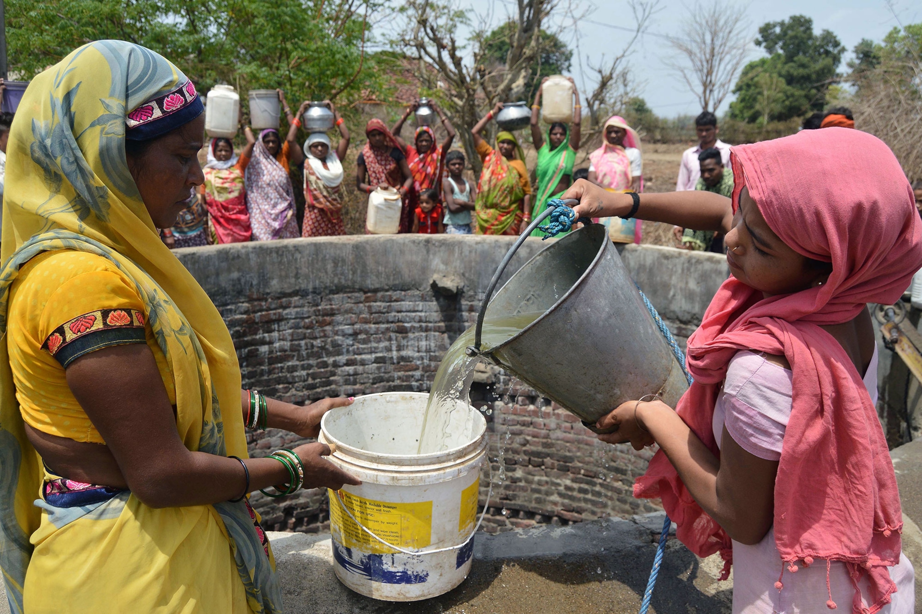
Women from the aboriginal Kol community collect drinking water at a well in Nawargawa village in Madhya Pradesh state on June 16, 2019. Around 40 families in the village rely on the well for drinking water during the heatwave conditions in the remote region in central India.

Buy me a river

Bangalore sits smack in the center of the lower half of the Indian peninsula, about 3,000 feet above sea level. A city of 12 million, one of the fastest growing in the world, it contributes $110 billion to India’s GDP. “Bangalore deserves to be water-secure,” says S. Vishwanath, director of Biome Environmental Solutions , a local design firm.

For Hungry Minds

Yet Bangalore has no perennial water source of its own. It has to pump water nearly 90 miles and up nearly 900 feet from the Cauvery, a sacred river that flows south of the city.

The city draws 1450 million liters per day (MLD), about 385 million gallons, from the Cauvery, with withdrawals slated to go up by 775 MLD (210 million gallons) in a couple of years, when new pipes will be laid. Still, the water does not reach everybody.

“Bangalore’s water woes are not as much a problem of supply, as it is of distribution,” Vishwanath says.

A quarter of Bangalore’s population, living mostly on its periphery, is not connected to the river water supply and is forced to mine groundwater to survive. This area of the city, replete with tech parks, is where most of the growth is.

Rampant groundwater extraction, unmonitored and unregulated, has caused Bangalore’s water table to plunge to depths of nearly 1,000 feet. Muddy and contaminated, the diminished resource threatens the future of the citizens who depend upon it.

Since in some places the groundwater is now below the level of the river itself, the river has begun to feed the groundwater. The Cauvery is thus being sucked dry from two sides—by the giant pipes that pump water into the city and by the bore wells that drive deeper each year, lowering the water table to levels below that of the river and forcing the river to feed it.

Water is pumped from the Bendsura reservoir to a tanker in this aerial photograph taken in Beed district, Maharashtra, India, on Sunday, Apr. 14, 2019.

Unreliable supply

Here’s what’s most unsettling: Bangalore’s current water distribution problems could evolve into a fundamental crisis of supply, because flows in the life-giving Cauvery are no longer secure.

Climate models predict a 5 percent increase in the river’s flow due to rising temperatures, which should bring more evaporation and heavier rains. However, that is not what recent trends in the basin show. Instead, dry season flows from the upstream regions of the river have been declining.

“These models don’t seem to be able to explain the recent past,” says hydrologist Veena Srinivasan, Fellow at the Ashoka Trust for Research in Ecology and the Environment (ATREE), Bangalore. The problem, she says, is that the models are not yet powerful and sophisticated enough to incorporate the effects on climate and weather of local changes in the landscape.

There have been plenty of changes. In the catchment regions of the Cauvery, widespread clear-cutting of forests to make way for transmission lines, coffee and palm-oil plantations, and other cash crops has affected the soil’s ability to retain and release water.

Research has also shown that large-scale deforestation affects South Asia’s monsoon, depressing precipitation levels—because fewer trees means fewer leaves transpiring water back to the atmosphere, resulting in warmer and drier conditions.

According to a study done by Coffee Agroforestry Network (CAFNET), this region has seen a decrease of 14 rainy days a year over the past three to four decades. Moreover, agricultural land-use has also changed near the river, with traditional paddy-fields giving way to coffee plantations. Paddy, with its requirement for standing water, meant that the fields traditionally acted as a spongesa sponge. Coffee and palm-oil plantations, in contrast, require heavy irrigation and see significant run-off.

“We don’t seem to be connecting the dots,” says Harini Nagendra , professor of sustainability at Azim Premji University in Bangalore. “Instead of trying to get more water into the Cauvery, we are investing time in fighting over its dwindling resources.”

If the Cauvery is dwindling, and groundwater is near exhausted, what options does Bangalore have?

First, catch the rain

Bangalore gets between 800 and 900 millimeters (32-36 inches) of rain in a year, which is hardly a meager amount. If the city were to catch half of that, it would translate to more than 100 liters (27 gallons) per capita per day, far more than adequate for domestic and drinking purposes. Rainwater harvesting has been slow to catch on in the city, in spite of laws requiring it, but it’s now steadily picking up.

You May Also Like

The deceptively simple plan to replenish California’s groundwater

Here’s what worries engineers the most about U.S. infrastructure

These cities are sinking into the ground

The next step would be to funnel some of the harvested rain via “recharge wells” back into groundwater, to begin to restore it. Two Bangalore NGOs, Biome Environmental Trust and Friends of Lakes, have launched a citizens’ initiative to dig a million recharge wells in the city—that’s about one every 90 feet. The idea is that these wells will pump back 60 percent of the rainwater into the shallow aquifer that has been depleted by overuse—and by the fact that only around 10 percent of rainwater currently can seep through cracks and gaps in the city’s pavement.

A local community of well-diggers called the mannu-vaddars man the effort. Using hand toolstools, they dig 30-to-40-foot-deep open wells that strike the shallow aquifer. Once it has been recharged the wells themselves become sustainable and cheap water source.

Vishwanath has other plans for recharging groundwater. Bangalore returns about 80 percent of its water to rural areas in the form of wastewater that flows in seasonal streams and rivers. Much of it is untreated—putrid, dark, and thick with sewage and hazardous heavy metals.

“Waste treatment plants are being put in place to treat 1440 MLD,” says Vishwanath. Once that begins to function, ‘fit for purpose’ water, cleaned of heavy metals but still rich in nutrients like phosphorus, will be returned to rural areas for use in agriculture. Vishwanath’s idea is to treat some of the wastewater further, to render it potable, and use that to recharge groundwater.

There is one gaping hole in the hopeful vision evoked by these ideas: India’s woeful lack of the institutions and governance needed to oversee such efforts and manage the water supply soundly, according to rules that are enforced.

A Chennai resident fills a pot with water from a tap on June 26, 2019. Chennai is getting less than two-thirds of the water it normally uses each day.

In Bangalore, the governmental department that oversees groundwater extraction has just six employees, and thus no earthly way to monitor and enforce the law in this sprawling city. One digger of illegal borewells freely admitted to me that he had paid a bribe to get a permit for a deep well—after he had already dug it.

At the larger river-basin level, there are no institutions in place to manage water resources at all.

“We are all fixated on technological solutions to the water crisis,” Vishwanath laments. “What we really need are robust institutions and governance at the river basin level so that we can understand what is happening to land-use change, sand-mining, forest cover, and groundwater extraction—all of which affects river flows.”

Without strong government involvement, known solutions to India’s water crisis won’t be implemented at a large enough scale to affect the bigger picture. Chennai is a case in point.

Chennai’s fossil water addiction

With a GDP of $78 billion, home to 40 percent of India’s automobile industry, Chennai has boxed itself into a corner as far as water resources go. Located on the east coast, it gets two-thirds of its rains from the northeast monsoon that arrives in November and December and only a third from the southwest monsoon—the one that this year has been less than enthusiastic.

The city depends on four small municipal reservoirs; it doesn’t have access to larger reservoirs, shared with agriculture, that it can borrow water from in a drought. Moreover, these four reservoirs service only 35 percent of the city’s water needs. Seven of 11 million people in Chennai depend upon fossil groundwater, w accessed either by privately dug borewells or by tank trucks that bring water in from distant borewells. The tankers are controlled by powerful water-mafias.

“The state [controlling only 35 percent of the water supply] becomes the minority, and its influence gets subverted as private [tanker] interests have captured value addition in water. They run it like a business,” says Vishwanath. The water mafias are well-connected to politicians, bureaucrats, and the police, making them difficult to dislodge. With taps running dry, voices are getting shrill and the government, as a band-aid measure, has set aside ten million dollars for a 50-wagon train to ferry 10 million liters (about 3 million gallons) of water every day from the Cauvery to Chennai.

Chennai, like many cities in India, has built over its wetlands . The pavement prevents groundwater from being recharged during rainy months—and instead causes low-lying areas to flood.

A man walks along a water pipe on the bottom of the dried-out Porur Lake in Chennai on Friday, July 5, 2019. Failed rains last year and delays in this year's annual monsoon have left nearly half of India facing drought-like conditions.

“The increasingly short attention span of policy makers, decision makers, the media, and even of citizens is frightening,” Nagendra says. “We focus on drought issues in the summer, and forget them once the monsoon strikes. We then focus on the challenges of too much water via flooding, and again forget this when the summer hits. Ironically the causes are much the same for both drought and floods—loss of wetlands, cutting of trees, building over lakes, rivers and interconnecting channels. But no one seems to make the link.”

The problem is nationwide; Chennai and Bangalore are just the leading edge. “The real crisis will come in the smaller cities and towns that are now fast urbanizing,” Nagendra says. “And the real hope of doing something may also lie there, as many of these areas have not yet faced ecosystem degradation and collapse at the scale that megacities have.”

Srinivasan is optimistic even for the degraded megacities.

“In a city with urban sprawl, the water problem is eminently solvable,” she says. “You build out your infrastructure for rainwater harvesting, you recharge the aquifers with treated wastewater, and make sure paving has enough give for rainwater to seep through.”

If India can just build the institutions to do all that, there will indeed be hope.

Related Topics

• GROUNDWATER
• FRESH WATER
• WATER QUALITY
• WATER CONSERVATION

Europe’s water crisis is much worse than we thought

The delicate art of catching fog in the desert

Japan releases nuclear wastewater into the Pacific. How worried should we be?

England’s chalk streams were millions of years in the making. Can they survive today?

The U.S. plans to limit PFAS in drinking water. What does that really mean?

• Environment
• Perpetual Planet

History & Culture

• History & Culture
• History Magazine
• Mind, Body, Wonder
• Paid Content
• Terms of Use
• Privacy Policy
• Your US State Privacy Rights
• Children's Online Privacy Policy
• Interest-Based Ads
• About Nielsen Measurement
• Do Not Sell or Share My Personal Information
• Nat Geo Home
• Attend a Live Event
• Book a Trip
• Inspire Your Kids
• Shop Nat Geo
• Visit the D.C. Museum
• Learn About Our Impact
• Support Our Mission
• Advertise With Us
• Customer Service
• Renew Subscription
• Manage Your Subscription
• Work at Nat Geo
• Sign Up for Our Newsletters
• Contribute to Protect the Planet

Copyright © 1996-2015 National Geographic Society Copyright © 2015-2024 National Geographic Partners, LLC. All rights reserved

Living with droughts

As per a Global Assessment Report on Disaster Risk Reduction: Special Report on Drought 2021 , released by the UN Office for Disaster Risk Reduction (UNDRR) recently “the impact of severe droughts on India’s GDP is expected to be about 2-5% per annum, despite the decreasing contribution of agriculture in the country’s expanding economy.”

India’s economy is rightly called the ‘gamble of monsoon’ and the arid and semi-arid regions in the western, northern and peninsular parts experience more frequent droughts, a slow-onset disaster.

Droughts have deep impacts on societies, ecosystems and economies. The costs are borne disproportionately by the most vulnerable people. As per UNDP, the impact of severe droughts as in 2002 includes large-scale ecological damage, mass migration and death.

“The extensive impacts of drought are consistently underreported, even though they span large areas, cascade through systems and scales, and linger through time. They affect millions of people and many sectors and domains -- such as agricultural production, public water supply, energy production, waterborne transportation, tourism, human health and biodiversity -- contributing to food insecurity, poverty and inequality,” says the report.

In fact, in north-west­ern India, a combination of drought and groundwater overabstraction led to decreasing trends in groundwater levels and reduced resilience to future droughts (Pathak and Dodamani, 2019).

Impact of climate change

"Climate change is increasing temperatures and disrupting rainfall patterns, thus increasing the frequency, severity and duration of droughts in many regions. As the world moves towards being 2°C warmer, urgent action is required to better understand and more effectively manage drought risk to reduce the devastating toll on human lives and livelihoods," says the report commissioned by the UNDRR.

The report which incorporates inputs from the World Meteorological Organization (WMO) notes that the number of droughts will grow dramatically because of climate change, environmental degradation and demographic shifts. This will pose a threat to the achievement of the Sendai Framework for Disaster Risk Reduction, the Sustainable Development Goals and human and ecosystems health and wellbeing.

The biggest impacts of climate change have to do with water. Urgent action is therefore needed to improve drought management and prevention, such as through the development and the strengthening of Multi-Hazard Early Warning Systems (MHEWS) to enable multi-hazard, all-media emergency alerting. Impact based MHEWS help societies to prepare for, and respond to, all types of disasters, including those related to hydrometeorological hazards.

As drought is a slow onset event, early warning and alerting offers opportunities to enhance collective action that can save lives and minimize potential economic and environmental damages. A powerful way to adapt to climate change is to invest in early warning services and meteorological and hydrological services.

Case study: India

The report has a section on case studies that explores the countries’ capacities to respond to drought-related impacts vary. They highlight how limited knowledge on possible impacts, poor assessments of vulnera­bilities and costs, little coordination at national and regional levels, and lack of awareness on policy options are key impediments to effective drought management.

The India case study highlights the Deccan Plateau region (about 43% of southern and eastern India), which has faced major drought conditions in recent times in 2000–2003 and 2015–2018. Significant drought conditions occur once in 3 years (Mishra and Singh, 2010).

Rainfed agriculture is the dominant source of food production in this low rainfall area where droughts are embedded into society and the economy. “In terms of drought preparedness in agri­culture, crisis management plans and drought contingency plans are prepared each season, which, to varying extents, connect with coping strategies at farm level (e.g. choice of crop variety),” the report says.

The water demands of rapid urban­ization and industrialization in recent years have seen groundwater systems dry up without appro­priate aquifer replenishment.

Also, in India drought-related decisions and policies are made at national and state levels, the centre being the main authority and “drought declaration” being the most import­ant step in governmental response to a drought situation. However, institutions treat drought as discrete, episodic and outlier events, choosing to respond only when drought emergencies arise. This leads to perpetuation and aggravation of drought vulner­abilities, agrarian crisis and natural resources degradation.

The key aspects discussed in the India case study were drought impacts and risk governance; substantial variance in the quality of drought monitoring; exacerbation of pre-existing vulnerabilities during droughts. The case study notes that monitoring, early warning and technical improvements to drought manage­ment systems – ongoing and planned – need to focus on “practical” tools that can be embedded and sustained in operational systems that capture the dynamic vulnerability and strengthen existing systems.

“The hazard posed by drought can be compounded by exacerbating effects such as the co-occurrence of droughts and heatwaves, antecedent soil moisture deficits and the feedback and connections among droughts, heatwaves, wildfires and even floods,” as per the report.

Key recommendations

Addressing the full complexity of drought and reducing risk will require partnerships, greater public awareness and support, and participation and action at all levels.

The report calls for proactive and innovative approaches to drought risk management -- reflecting the long-held view of WMO which has campaigned for more proactive, coordinated and sustainable management policies to replace the current crisis-driven piecemeal response.

The report recommends the establishment of new coordination and collaboration mechanisms to rapidly advance the understanding and management of drought risk. This is the philosophy behind  WMO's Integrated Drought Management Programme  which is based on the  three pillars of monitoring and early warning; vulnerability and impact assessment; drought risk mitigation, preparedness and response .

Specific recommendations include -

• Prevention has far lower human, financial and environmental costs than reaction and response.
• Increased understanding of complex systemic risks and improved risk governance can lead to effective action on drought risk.
• Drought resilience partnerships at the national and local levels will be critical to managing drought in a warming world where rainfall will become ever more unpredictable and require practical solutions to tackle issues like deforestation, excessive use of fertilizers and pesticides, overgrazing, salination, waterlogging and soil erosion.
• A mechanism for drought management at the international and national levels could help address the complex and cascading nature of drought risk.
• Financial systems and services need to evolve to encourage cooperative approaches, to promote social protection mechanisms and to encourage risk transfer and contingent financing, so as to provide diversified adaptive support to drought risk management.

Click through the PLOS taxonomy to find articles in your field.

For more information about PLOS Subject Areas, click here .

Loading metrics

Open Access

Peer-reviewed

Research Article

Drought and temporary migration in rural India: A comparative study across different socio-economic groups with a cross-sectional nationally representative dataset

Roles Conceptualization, Data curation, Formal analysis, Methodology, Writing – original draft, Writing – review & editing

* E-mail: [email protected]

Affiliation Department of Policy and Management Studies, TERI School of Advanced Studies, New Delhi, NCT of Delhi, India

Roles Conceptualization, Writing – review & editing

Roles Conceptualization, Methodology, Writing – review & editing

Affiliation Division of Preventive Oncology & Population Health, National Institute of Cancer Prevention and Research, Indian Council of Medical Research, Noida, Uttar Pradesh, India

• Badsha Sarkar, 
• Swarup Dutta, 
• Prashant Kumar Singh

• Published: October 7, 2022
• https://doi.org/10.1371/journal.pone.0275449
• Reader Comments

Vast stretches of India comes under meteorological drought this year or the other. A huge population base in rural India are rendered highly vulnerable to this drought because of their primary dependency on agriculture and in turn they may respond through temporary migration out of the drought affected rural areas in search of alternative livelihoods. This study aims to investigate the association between drought and temporary migration in rural India by fitting binary logistic regression models on a cross-sectional dataset involving both National Sample Survey Organization (NSSO) 64 th round data and India Meteorological Department (IMD) rainfall data. The paper also examines whether this association varies across the different socio-economic groups. Out of the total temporary migrants generated in rural India in the study period, 99.46% migrated internally and 67.12% were rural to urban migrants. The study finds that there is a positive association between drought instances and probability of a household to have at least one temporary migrant member in rural India (OR 1.64 with p<0.001) while controlling all other covariates. The study also concludes that the probability of temporary migration on account of drought is more severe among the socio-economically marginalised sections of the rural population compared to their better-off counterparts.

Citation: Sarkar B, Dutta S, Singh PK (2022) Drought and temporary migration in rural India: A comparative study across different socio-economic groups with a cross-sectional nationally representative dataset. PLoS ONE 17(10): e0275449. https://doi.org/10.1371/journal.pone.0275449

Editor: Md Nazirul Islam Sarker, Neijiang Normal University, CHINA

Received: January 13, 2022; Accepted: September 15, 2022; Published: October 7, 2022

Copyright: © 2022 Sarkar et al. This is an open access article distributed under the terms of the Creative Commons Attribution License , which permits unrestricted use, distribution, and reproduction in any medium, provided the original author and source are credited.

Data Availability: The data underlying the results presented in the study are based on National Sample Survey Organisation (NSSO) 64th round available from: http://www.icssrdataservice.in/ after registration.

Funding: The first author is registered under a PhD program which earlier was supported by UGC NET JRF scheme of Government of India.

Competing interests: The authors have declared that no competing interests exist.

Introduction

India is a highly drought affected country. The percentage area under drought in the country has increased from 10% to 20% during the period 1959 to 2009 [ 1 ] along with an increase in intensity of monsoon droughts [ 2 – 4 ]. India is projected to face an increasing future trend of droughts which will be more severe, frequent, long and with greater spatial extent under warming climate scenarios [ 5 , 6 ]. Characteristics such as high levels of poverty, high levels of borrowing, less crop diversity, agriculture as the major source of income and low level of agricultural insurance increase people’s vulnerability to drought [ 7 ]. Drought causes decrease in grain yields [ 8 , 9 ]. One fifth of India’s population are living below international poverty line [ 10 ] and half of its population are still dependent on agriculture and these make the Indian population vulnerable to drought. Impacts of droughts can be felt across economy, environment and society. The most immediate socio-economic impacts of droughts are manifested in widespread disruption in rural societies on account of livelihood insecurity, greater indebtedness, reduction in the consumption of cereals, rise in school dropout rates, psychological and health problems, loss of social status among the most vulnerable sections, increase in social tensions and erosion of social capitals including outmigration of the population from the drought affected regions [ 11 – 13 ]. In the year 2020 alone, around 3,856,000 people were estimated to be internally displaced in India due to disasters including droughts [ 14 ].

The association between drought and human migration has been studied in many regions around the world including Brazil [ 15 ], Canada [ 16 , 17 ], China [ 18 ], Ethiopia [ 19 , 20 ], Kenya [ 21 ], Mali [ 22 , 23 ], Nepal [ 24 ], Northern Latin America and the Caribbean [ 25 ], Syria [ 26 ], United States of America [ 27 ] etc. In India, a few studies have found a positive association between drought and migration by analysing Census of India and International Crops Research Institute for the Semi-Arid Tropics (ICRISAT) datasets [ 28 – 30 ]. This association between drought and migration is also evidenced in a few field based studies spread across different parts of India like Karnataka [ 31 ], Odisha [ 32 – 34 ], Tamil Nadu [ 35 ], West Bengal [ 36 , 37 ], Hindu Kush-Himalayas [ 38 ] etc. This drought and migration nexus may vary across the different intersectional groups based on their different levels of access to resources and the different adaptation strategies adopted. A number of studies informs that the socio-economic backgrounds play an important role while taking decisions regarding migrations in the instances of drought or any other natural hazards in India [ 7 , 32 , 33 , 35 , 36 , 39 – 42 ]. On this background, this study aims to investigate the association between drought and temporary migration in rural India by employing secondary datasets and applying quantitative methods. The paper also examines whether this association varies across the different socio-economic groups. After this short introduction, the paper will describe the datasets and statistical models used in the study, followed by a description of results and discussions and finally will end up in a conclusion.

Materials and methods

Socio-economic data.

The socio-economic data source used for this study is from National Sample Survey Organisation (NSSO) 64 th round conducted between 1 st July 2007 and 30 th June 2008 called Employment and Unemployment and Migration Particulars with schedule 10.2 which is a nationally representative large sample survey. The survey was conducted under the aegis of National Sample Survey Office, Ministry of Statistics and Programme Implementation (MoSPI), Government of India (GoI). NSSO is in charge of carrying out extensive sample surveys across all over India. NSSO primarily collects data through national household surveys on numerous socioeconomic topics, Annual Survey of Industries (ASI) etc. In addition to conducting these surveys, NSSO gathers information on rural and urban pricing and contributes significantly to the advancement of crop statistics by supervising the area enumeration and crop estimating surveys conducted by state agencies. In addition, it keeps track of a frame of urban area units for use in sample surveys in cities. NSSO 64 th round is the latest available data on temporary migration from any government sources in India. The survey covered the whole of Indian Union except; Leh (Ladakh) and Kargil districts of Jammu and Kashmir, interior villages of Nagaland situated beyond 5km of the bus route and villages of Andaman and Nicobar Islands which remain inaccessible throughout the year. Data was collected from 12,589 first stage units (FSUs) - 7,921 rural and 4,668 urban—distributed over all the 35 states and union territories through a stratified multi-stage random sampling design. A sample of about 10 households was drawn from each selected village and urban block comprising a total 125,578 households (79,091 in rural areas and 46,487 in urban areas) and a total of 572,254 persons (374,294 in rural areas and 197,960 in urban areas). The data of this survey is available in public domain and can be accessed upon registration and request to ICSSR Data Service (available at http://www.icssrdataservice.in/ ). This source also contains more details about the sampling procedure of the survey. This study was approved by a Student Research Committee instituted by TERI School of Advanced Studies, New Delhi. Separate approval for conducting this research was not required since this study was based completely on secondary datasets generated by Government agencies and those datasets are freely available in the public domain.

Sample size for the study

The study is cross-sectional in design and the unit of analysis is household. As discussed above the total sample size at household level in NSSO 64 th round is 125,578 which reduces to 79,091 after deducting the urban sample. After deducting the non-reporting cases of religion (2), social group (6), land possession (66), marital status (4), and educational status (19) the household sample size at rural areas further reduces to 78,994 which constitutes the total sample size for this study. The study classifies this total sample size into 3 equal economic groups (based on Monthly Per capita Consumption Expenditure [MPCE] tertiles) of lower economic group (LEG = 26,316), middle economic group (MEG = 26,342) and higher economic group (HEG = 26,336). The same total sample size is again decomposed into 4 social groups of Others (19,512), Other Backward Class (OBC = 30,974), Scheduled Castes (SC = 15,085) and Scheduled Tribes (ST = 13,423).

Outcome variable

In this study a temporary migrant household is considered to be the dependent variable. To record data on temporary migration, NSSO 64 th round used the criteria of if a parson has stayed away from the place of enumeration for a continuous period of at least one month but less than six months during last one year for employment or in search of employment then that person is categorised as a temporary migrant. The present study codes a household with at least one temporary migrant member as 1 and a household without any temporary migrant member as 0. Out of the total temporary migrants in rural India, 99.46% migrated within national border and 67.12% were rural to urban migrants.

Key explanatory variables

The meteorological data used in this study are from India Meteorological Department (IMD) gridded rainfall binary files (0.25*0.25) (available at https://www.imdpune.gov.in/Clim_Pred_LRF_New/Grided_Data_Download.html ). Point level annual (1 st of January to 31 st of December) rainfall data were extracted with the help of GRADS 2.2 on yearly basis and were imported to QGIS 3.10.0 as shape files and interpolated (inverse distance weighted). All the data points falling within one district were averaged to get the annual rainfall data of that district. Districts which have experienced an annual rainfall negatively deviated by an amount of 40% or more than the normal rainfall (50 years average annual rainfall between 1951 to 2000 for that district [ 43 ]) for at least one year between five years preceding the NSSO survey i.e. between 2003 to 2007 [ 28 , 44 – 46 ] are classified as drought ( DR ) affected. If the district had no drought year within the specified time period then the district was coded as 1 and a district with at least one drought year was coded as 2. The districts with a positive deviation of rainfall of at least 40% or more within the specified time period of 2003 to 2007 were classified as flood ( FL ) affected. Drought and flood data were merged with the NSSO data at district level.

Other than the meteorological variables, other background characteristics like demographic, economic, social and geographical, which may influence a household to undertake a temporary migration decision, have also been considered in this study either as household characteristics or as household head characteristics. The selection of the covariates depends on both the literature [ 47 – 50 ] and availability in NSSO 64 th round dataset. The study has considered eight household characteristics including household size ( SIZE : up to 5 members and more than 5 members), whether the household has at least one non-resident (out-migrant) member ( OUT ), religion ( REL : Hinduism, Islam and Others), social groups ( SOCIAL : Others, Other Backward Class, Scheduled Castes and Scheduled Tribes), household land possession ( LAND : up to 1 hectare, 1.01 to 4 hectares and more than 4 hectares), household occupation type ( OCCU : self-employed in agriculture, self-employed in non-agriculture, agricultural labour, other labour and others), and MPCE categorised into 3 tertile classes with equal frequencies. The dimension of geographical variability was incorporated through the consideration of state of residence ( STATE ) with Bihar as the reference category. Four other variables have been employed to capture the characteristics of the household head as sex ( SEX : male and female), age ( AGE : 15–24, 25–34, 35–44, 45–54, 55–64, up to 14 & 64 and above), marital status ( MAR : currently married, never married, widowed, divorced/separated), and educational level ( EDU : not literate, literate but up to primary, above primary but up to secondary and above secondary). A more detail description of explanatory variables and their measurements are provided in S11 Table in S1 File . Pairwise correlation coefficient matrix shows that the r 2 values range between +6 to -6 (S1-S8 Tables in S1 File ).

Model specifications

Eq 2 describes the odds ratio in the form of probability of household i to have at least one temporary migrant member divided by the probability complement. A logarithm of the odds ratio makes the logistic regression model a function of different independent variables ( X i ) in Eq 3 where α denotes intercept, β denotes coefficients and ε i denotes the error term. Eqs 4 and 5 depicts more comprehensive forms of the binary logistic regression models for the study.

Data arrangement was done in SPSS 25 and Excel 13 and the regression models were built using STATA 15.

Characteristics of the overall sample

Out of the total sample size of 78,994 households, 15.6% had at least one member who undertook a temporary migration during the last year (see Table 1 for unweighted sample characteristics and S12 Table in S1 File for weighted sample estimates). An amount of 9.3% and 13.2% households belong to a district which had faced a drought and flood for at least once in the last five years respectively. In terms of household characteristics, almost 70% of households are composed of up to 5 members. There are about 46.4% households where already at least one member of the household had migrated out (non-resident). In terms of religious affiliation, 78.6% households are affiliated with Hinduism. Almost 3/4 th of households belong to one or the other reserved social categories. About four out of five households (80.7%) possess only up to 1 hectare of land. In majority of the households (50.6%) the major source of income is self-employment either in agricultural or in non-agricultural activities whereas 33.8% households bring their major source of income from selling labour. There are about one third households with MPCE level below Rs. 774.20. Majority of the households (84.9%) are male headed and 50% of the household heads are of 35–54 years age group. As per personal details of household heads, 85.3% are currently married and 41.3% are not literate. In terms of geographical distribution of the sample, number of states contributing more than 5% share in migration are 6 which are Uttar Pradesh (11.4%), Bihar (8.9%), Andhra Pradesh (7.1%), West Bengal (6.9%), Maharashtra (6.4%) and Madhya Pradesh (5.6%).

• PPT PowerPoint slide
• PNG larger image
• TIFF original image

https://doi.org/10.1371/journal.pone.0275449.t001

Temporary migration rates by key explanatory variables and covariates across different socio-economic groups

Cross tabulation between migration and drought does not give any conclusive relationship between the two (see Table 2 for unweighted temporary migration rates and S13 Table in S1 File for weighted sample estimates). Households in the MEG, HEG and SC categories who belong to drought affected districts show marginally higher rates of temporary migration. On the other hand, the households in the overall sample, MEG, HEG, OBC and ST when belonging to flood affected districts have higher rates of temporary migration. Temporary migration rates are higher for households with family size more than 5 members and households with no out-migrant members across all the samples. Households affiliated with Islam have higher migration rates in all groups except HEG and ST. The SCs have higher migration rates in overall sample as well as in LEG and MEG. Households with up to 1 hectare of land possession have the higher migration rates except in HEG and ST. Households whose main income source is labour (either agricultural or non-agricultural) have higher migration rates compared to entrepreneurial households. Households within the lowest MPCE group produce the higher rates of migration. Male headed households produce more migrants over female headed households. Households with household heads aging between 45–54 have higher migration rates except MEG. Households with currently married household heads and household heads with no literacy produce more migrants. Among the larger states, Jharkhand is the highest migration rate generating state in the overall sample (26.9%), LEG (33.2%), MEG (24.9%), OBC (25.4%) and SC (38.5%) categories whereas Bihar produces the highest migration rate in the HEG (16.6%), West Bengal in Others (23.6%) and Gujarat in ST (29.2%) category.

https://doi.org/10.1371/journal.pone.0275449.t002

Associations between household characteristics, household head characteristics, geographical variables and temporary migration across the different socioeconomic groups

Households with more than 5 members and households without any out-migrant member are associated with higher probability for migration in comparison to their respective counterparts across all the groups after controlling all the covariates (Tables 3 and 4 ). Households affiliated with Islam are more probable to migration in comparison to Hindus across all the samples except OBC (OR 1.05 with p = 0.323) and SC (OR 0.98 with p = 0.933) while controlling all the covariates. In the overall sample and across all the three economic groups, the socially marginalised households are more probable to have at least one migrant member when compared to socially better off sections except MEG. With the increase in household land possession size the probability of migration goes on decreasing. In comparison to households where the main income source is self-employment in agriculture, the households with self-employment in non-agriculture, agricultural labour and other labour have higher probability for migration. The likelihood of migration decreases with increasing MPCE tertiles. The probability for member(s) of female headed household to undertake migration as compared to male headed households is invariably low (at a p-value less than 1%) in all the categories with the highest being observed among the STs (OR 0.63 with p<1%). Households with heads aged between 45–54 years show higher probability for migration in overall sample (OR 1.15 with p<10%), HEG (OR 1.39 with p<5%) and Others (OR 1.51 with p<5%). In terms of marital status of household heads, widowed headed households have higher probabilities for migration compared to households headed by currently married persons except STs. Households with illiterate household heads have higher probabilities for migration compared to others. Across all the states the households belonging to Bihar show higher probability of migration across all the groups except for overall, HEG and ST. ST households belonging to Nagaland (OR 3.63 with p<1%), Jharkhand (OR 1.75 with p<5%), Assam (OR 1.72 with p<10%) and Gujarat (OR 1.68 with p<10%) are more likely to be mobile compared to Bihar. Nagaland also scores higher probability in the overall sample (OR 2.24 with p<1%) and the HEG (OR 2.11 with p<1%).

https://doi.org/10.1371/journal.pone.0275449.t003

https://doi.org/10.1371/journal.pone.0275449.t004

Association between drought and temporary migration across the different socioeconomic groups

There is a positive association between drought and temporary migration in the overall sample (OR 1.64 with p<1%) as well as among the socio-economically marginalised sections compared to their better off counterparts after controlling all the covariates (Tables 3 and 4 ). Households in the LEG have more than two times (OR 2.32 with p<1%) likelihood for having at least one temporary migrant member when they are based at a drought affected district in comparison to a district not affected by drought while controlling all other variables. This ratio decreases to one and half times (OR 1.55 with p<1%) for households belonging to the MEG and the association renders statistically insignificant when HEG is concerned. Among the households belonging to OBC, the probability for having at least one migrant member is almost two times greater (OR 1.95 with p<1%) when they belong to a drought affected district in comparison to a non-drought affected district. This ratio is 1.92 for SC and 1.59 for ST with less than 1% p-value. The association between drought and migration for the Others category households is statistically insignificant. The association between flood and migration is insignificant for all the categories except SC (OR 0.86 with p<10%) and ST (OR 1.74 with p<1%).

Robustness checks

For checking the consistency of the results of binary logistic regression models, multiple linear regression models were fitted onto the same datasets at household level. The results show that the direction of relationship still holds true in the simple OLS models but this time with lesser intensity (S9 Table in S1 File ). There is a positive association between drought and probability of a household to have at least one temporary migrant member (OR 1.05 with p<1%). This association holds positive for households in the marginal socio-economic categories like LEG (OR 1.17 with p<1%), MEG (OR 1.05 with p<1%), ST (OR 1.05 with p<1%), SC (OR 1.09 with p<1%) and OBC (OR 1.09 with p<1%) and statistically insignificant for HEG and Others.

Again datasets were prepared for the individual level (rather the household level which has been the unit of analysis till now) for age group 15–64 and binary logistic regression models were fitted (S10 Table in S1 File ). At individual level analysis almost the similar relationships between drought and migration hold true as seen for the binary logistic regression models at household level. Drought is positively associated with migration for the overall sample (OR 1.69 with p<1%) and also for the marginalised socio-economic classes of LEG (OR 2.36 with p<1%), MEG (OR 1.52 with p<1%), ST (OR 1.76 with p<1%), SC (OR 1.81 with p<1%) and OBC (OR 1.90 with p<1%) and not significant for HEG and Others.

The criteria for drought definition for the study is set till now as at least 40% negative deviation in the annual rainfall from the normal rainfall for the district. Household level binary logistic regression models were also constructed for other measures of drought with 10% to 60% negative annual rainfall deviations at every 5% intervals. Other than 40% negative annual rainfall deviation measure of drought, the only other measure which produces statistically significant relationships between drought and temporary migration is 35% negative annual deviation but this time with lesser intensity.

The study investigates the association between drought occurrence and probability of a household to have at least one temporary migrant member with NSSO 64 th round data and IMD data fitted into quantitative models. This is one of the few studies especially on the Indian population where association between temporary migration and a specific natural hazard (here drought) has been investigated as against the dominant trend of using one or the other constructs of climate change or climate variability [ 30 , 52 , 53 ]. This association has been assessed at household level and across the different socioeconomic groups in rural India after combining the objective meteorological data from IMD with NSSO sample survey data. Out of the total temporary migrants in rural India, 99.46% migrated within the national border and 67.12% were rural to urban migrants. The study reveals a strong association between occurrence of drought and the probability of a household having at least one temporary migrant member. This finding is consistent with a study [ 28 ] which has found that drought frequency in the origin state brings with it an increase in the inter-state migration in India by analysing Census of India data 1991 and 2001. Again both the studies did not find any statistical association between flood (“excess precipitation”) and migration. A similar finding also has come up from another study [ 29 ] which with the exploration of ICRISAT cross-sectional data of 2013–14 found that climatic risks (which was reported to be heavily related to drought) brings an increase in the probability of migration in semi-arid parts of India. Real and futuristic migration intentions data may produce somewhat contradictory associations with drought as one study [ 54 ] employing perceived increased severity of drought and future migration intentions, has reported a negative association between the two.

The positive association between drought and migration may be explained with the help of conceptual frameworks proposed in the literature time to time. Migration may be influenced by a range of drivers including economic, social, political, demographic and environmental [ 47 ]. Drought may either directly influence migration through squeezing the ecosystem services (like increasing water shortages [ 55 ]) or through manipulating the other drivers of migration (like decreasing crop yield [ 8 , 9 ] or through intensifying social conflicts and decaying local social capitals [ 56 ]). These cumulative effects of drivers being filtered through other personal, household/community level factors may produce a migration. Another contribution of the study is the consideration of household as the unit of analysis. As per one of a theoretical strands of New Economics of Labour Migration [ 57 ] a household may distribute its workforce across diversified geographies/sectors as a risk aversive insurance strategy as if one geography/sector suffers from any crisis, the remittances from the other geography/sector(s) may keep the household going.

The study reveals a variation in the association between drought and migration across different socio-economic groups where socio-economically marginalised households have more probability for migration than their socio-economically better-off counterparts. This finding is consistent with a few field-based studies which point out that the decisions of migration and non-migration during the instances of droughts are very much influenced by the different socioeconomic backgrounds of the people in India [ 7 , 32 , 33 , 35 , 36 , 39 , 40 , 42 ]. An explanation through the lens of intersectionality may produce some relevant interpretation in this regard. An intersectional analysis illuminates how different households and groups relate differently to drought, due to their situatedness in power structures based on context-specific and dynamic social categorisations [ 58 ]. Drought may be experienced differently by different socioeconomic groups based on their different sets of resource availability and different adaptation/coping strategies. For relatively better socially and/or economically endowed households in-situ adaptation may be more preferred, but for poorly endowed households migration may be a result of failure to adapt in-situ or migration itself may be an opportunity for adaptation to drought if planned properly [ 59 ].

An examination of the association between temporary migration and covariates reveals that temporary migration as a livelihood strategy is highly concentrated among the socioeconomically marginalised sections of Indian rural population. It is the households belonging to marginalised social groups, households with smaller land possessions, households with main income source from agricultural labour and other labour, households with lower MPCE levels and households having illiterate heads are the ones with greater probability for having temporary migrant members. Various previous studies also had come up with similar findings [ 36 , 49 , 50 , 60 – 64 ]. Mere the occurrence of these socioeconomic drivers of temporary migration (i.e. belonging to marginalised sections) may not be enough to cause temporary migration to happen. There are certain other household characteristics or prerequisites which may facilitate a household to undertake a decision on temporary migration that this study has identified like households with more than 5 members, households without any out-migrant member, households affiliated with Islam, male headed households, households with head aged between 45–54 years and widowed headed households. It may be argued that having a minimum household size may facilitate a household to retain enough workforce at home while a section of it goes out of the village temporarily. Many of these prerequisites of migration have also come up in other studies from time to time [ 47 , 65 ].

The states of Uttar Pradesh, Andhra Pradesh, Bihar, West Bengal, Maharashtra etc. are the home to rural population who majorly belong to socioeconomically disadvantaged sections and this makes these states greater contributor of temporary migrants in India. Deprivations in the historical lines as well as lacuna in the present policy interventions may explain the production and reproduction of marginality in rural areas of these states. One of the processes of creating marginalisation may be exclusion from the traditional livelihood asset base like forest evection especially in the case of ST population [ 66 ]. In contrast to permanent and semi-permanent migrants who are drawn from more affluent parts of the community, temporary migration is mostly used by this impoverished and deprived socioeconomic segments of the Indian population as a technique to alleviate poverty [ 67 ]. However, temporary migration continues to be a costly and risky endeavour in terms of both tagibilities and intangibilities [ 65 , 68 ]. This may be the reason why initiatives to increase rural employment, like NREGA, may be able to reduce temporary migration even if they only compensate part of the economic benefits gained through temporary migration [ 69 ]. However, a few research also suggest that temporary migration is not just a survival strategy of poor people [ 70 , 71 ]. They contend that temporary migration can act as both a shelter of liberation and a path towards accumulation.

The study is not without limitations. Absence of any recent government dataset on temporary migration made the analysis dependent on a dataset (NSSO 64 th round) which was surveyed 13/14 years back and this may be the prime limitation of the study. One of the important limitations are related to the measurement issues of both migration and drought. The definition of temporary migration used in NSSO is restricted only to a very short time duration (away from the village for 1 month or more but less than 6 months during last 365 days) where a relaxation of time may have included a much broader picture. Consideration of more advanced measurements of drought in terms of Standardised Precipitation Index (SPI) or Standardised Precipitation Evapotranspiration Index (SPEI) or consideration of soil moisture drought or agricultural drought would have provided a more grounded analysis. Another dimension of measurement issue is the temporal discrepancy between drought and migration as drought is measured on a yearly basis which ranges between 1 st of January to 31 st of December and migration between 1 st of July to 30 th of June. One important limitation about model specification is absence of pull factors. The type of econometric model used in the study makes the results limited to correlational conclusions only rather than causation between drought and temporary migration. Some more advanced econometric models like instrumental variable models or structural equation models may serve this purpose. Here one thing needs mentioning is that in the study almost half of the districts affected with drought are concentrated in a single state of Tamil Nadu itself as the state was hit by a severe drought in 2003. A different geographical pattern of drought may have produced a different drought migration nexus. It is out of scope for this analysis to say whether this temporary migration in relation to drought is forced (displacement) or voluntary (planned migration). Again its also not possible to say whether this migration is an adaptation to drought or a failure to adaptation to drought as for this type of conclusions impact data of migration needs to be analysed.

The study finds that there is a positive association between drought instances and the probability of a household to have at least one temporary migrant member in rural India by fitting binary logistic regression models on a dataset involving NSSO 64 th round data and IMD rainfall data while controlling all other confounding variables. The study also concludes that the probability of temporary migration on account of drought is more among the socio-economically marginalised sections of the society compared to their better-off counterparts.

Supporting information

https://doi.org/10.1371/journal.pone.0275449.s001

Acknowledgments

The authors acknowledge the comments made by Dr. Seema Sangita and Dr. Montu Bose on the previous versions of this research. The comments of the academic editor and the four reviewers are also acknowledged.

• View Article
• Google Scholar
• 4. Pai D, Guhathakurta P, Kulkarni A, Rajeevan M. Variability of meteorological droughts over India. In: Nayak MNR, editor. Observed climate variability and change over the Indian Region. Singapore: Springer; 2017. p. 73–87.
• PubMed/NCBI
• 33. Panda A. Climate change, drought and vulnerability: A historical narrative approach to migration from Western Odisha, India. In: Rajan SI, Bhagat RB, editors. Climate change, vulnerability and migration. London: Routledge India; 2017. p. 193–211.
• 34. Sahu BK. Migration and household labor use for adopting climatic stress: A study of drought-affected areas in Odisha. In: Sarap DNR, editor. Rural labour mobility in times of structural transformation. Singapore: Palgrave Macmillan; 2017. p. 237–68.
• 37. Raha S, Gayen SK. Drought-induced human mobility in Purulia district of West Bengal. In: Rukhsana , Haldar A, Alam A, Satpati L, editors. Habitat, ecology and ekistics: Advances in Asian human-environmental research. Cham: Springer; 2021. p. 263–77.
• 40. Korra V. Dynamics of distress seasonal migration: A study of a drought-prone Mahabubnagar district in Telangana. In: Rajan SI, Bhagat RB, editors. Climate change, vulnerability and migration. 1st Edition. London: Routledge India; 2017. p. 212–36.
• 43. IMD. Rainfall Statistics of India– 2017. India Meteorological Department, 2018 ESSO/IMD/HS/Rainfall Report/01(2018)/24.
• 51. Gujarati D, Porter D. Basic econometrics. 5th ed: The McGraw− Hill Companies; 2008.
• 67. Bhagat RB, Keshri K. Internal migration in India. In: Bell M, Bernard A, Charles-Edwards E, Zhu Y, editors. Internal migration in the countries of Asia. Cham: Springer; 2020. p. 207–28.

South India’s Two-Year Drought From 2016 Was Worst In 150 Years, Study Finds

DMK party workers stage a protest over the water crisis in Tamil Nadu in Chennai, June 24, 2019. Photo: R. Senthil Kumar/PTI

Southern India was hit by severe drought from 2016 to 2018 arising from low rainfall during the northeast monsoon, which occurs during the winter. So severe was the impact that a water crisis erupted in Chennai, India’s sixth-largest city of 11 million inhabitants, as four of the city’s major reservoirs went bone-dry and groundwater levels plummeted. In the summer of 2019, a “Day Zero” was declared and residents scrambled to obtain water from tankers.

Now, after examining rainfall data over the past 150 years, researchers in India and the US conclude that the 2016-2018 northeast monsoon drought was unprecedented with more than 40 percent deficit in northeast monsoonal rainfall during the three years.

The recent drought was worse than the Great Drought of 1874-1876, which led to crop failure and which in turn resulted in the Great Madras Famine of 1876 to 1878, claiming millions of lives. The team demonstrates that cool phases in the equatorial Indian and Pacific Oceans are associated with the rainfall deficit.

“The consecutive failure of the northeast monsoon can result in a water crisis in Southern India,” lead author Vimal Mishra, associate professor at Indian Institute of Technology, Gandhinagar, told Mongabay-India, adding that “it has considerable implications to agricultural productivity.”

While India receives most of its annual rainfall during the Indian summer monsoon (June to September), southern India receives about 40 percent of its rainfall from October to December in what is known as the northeastern monsoon (NEM) or the winter monsoon. It is crucial for drinking water and agriculture contributing to the livelihood of millions.

The southern Indian states of Andhra Pradesh, Karnataka and Tamil Nadu continuously declared drought from 2016 to 2018 linked to low northeast monsoonal rainfall. Over 60 percent of the rural population in southern India is engaged in agriculture and relies on rainfall from the winter monsoon.

Failure of northeast monsoon 

How severe was the recent drought compared to those Southern India has experienced in the past? What are the causes of the deficit in the northeast monsoon? Mishra’s team sought to answer these questions.

To investigate the long-term history of NEM droughts in the region, the team used rainfall observations from the India Meteorology Department from 1870 to 2018. Data on total water storage was obtained from NASA’s Gravity Recovery and Climate Experiment (GRACE) satellites for April 2002 to June 2017 while the GRACE Follow-On (GRACE-FO) mission provided data for 2018 onwards.

Over the past 150 years, there were five main periods of drought with more than 29 percent deficit in rainfall (1876, 2016, 1938, 1988, and 1974 in order of severity). Looking at single year rainfalls, 1876 was the driest year with a precipitation deficit of 69 percent followed by 2016 with a deficit of 63 percent. But when considering cumulative rainfall over three years, 2016 to 2018 was the worst NEM drought with a precipitation deficit of 45 percent while the 1874 to 1876 drought, or the Great Drought as it is known, was the second-worst with a deficit of 37 percent.

The GRACE satellite indicated that total water loss in Southern India in December 2016 was 79 cubic kilometres (km3) while the GRACE-FO data showed that the loss was 46.5 km3 in June 2017 and 41.7 km3 in June 2019. Loss in total water storage likely resulted in significant depletion of groundwater in the region, say the authors.

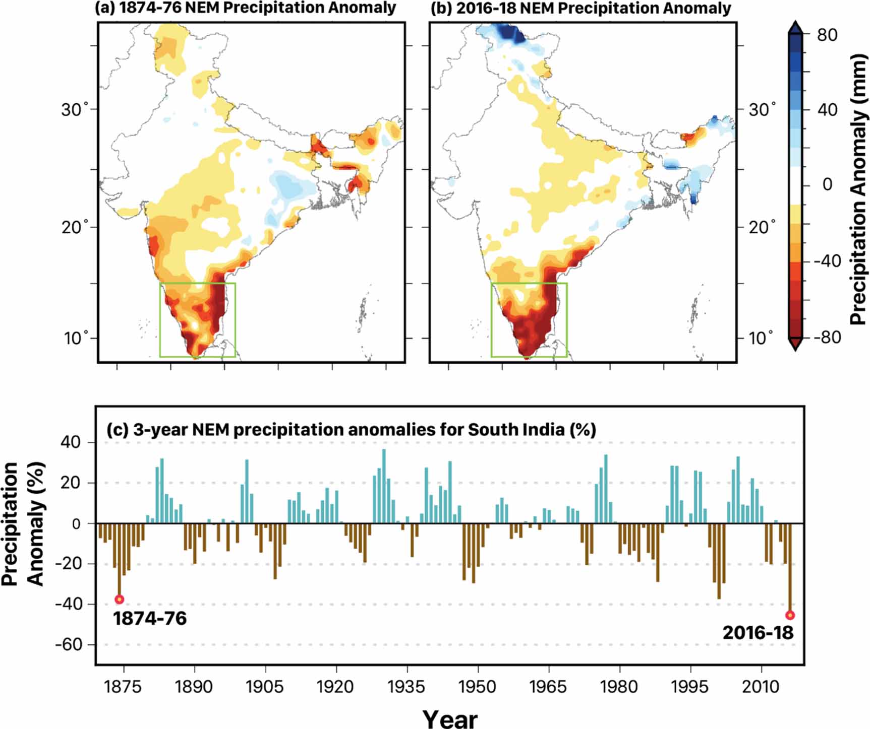
Associated factors

The team examined sea surface temperatures (SST), sea-level pressure and wind fields during the winter monsoon to understand how circulation patterns affect variability in northeast monsoonal rainfall. Sea surface temperature over the equatorial Indian and Pacific Oceans affects year-to-year variability of the northeast monsoon, explained Mishra. “SST anomalies cooler than normal are linked to a weak northeast monsoon.”

In 2016 and 2017, cool SST anomalies prevailed in the tropical Indo-Pacific Ocean and were associated with La Niña in the central Pacific, the researchers observed. La Niña is a climate pattern that occurs irregularly every two to seven years. During La Niña, the surface waters over the equatorial Pacific Ocean are cool and this affects global weather patterns.

At the same time, the researchers noted anomalous cooling was seen in the Indian Ocean. Such patterns along with those seen in sea-level pressure and surface-air temperatures gave rise to anomalous westerlies in the equatorial Indian Ocean, which weakened moisture transport from the Bay of Bengal during the northeast monsoon, explained the authors.

Interestingly, the study revealed that out of five of the major droughts that struck southern India over the past 150 years, four occurred during La Niña.

Deepti Singh, assistant professor at Washington State University, who was not connected with the study, notes that the paper “links the recent severe, multi-year drought primarily to La Niña conditions in the tropical Pacific Ocean in 2016-2017 and 2017-18.”

This finding “implies that there is potential to predict them a few months in advance since La Niña events can be predicted with some skill in the summer,” said Singh, adding that “this means that stakeholders can prepare for and mitigate their impacts.”

While the study does not explain what made the 2016-2018 drought one of the strongest on record, “it demonstrates that natural climate variability can lead to extreme events.” She stresses that a better understanding of these drivers can inform our ability to predict severe droughts in the future. “Timely predictions of such events can help better manage and potentially reduce their societal impacts,” Singh says.

“This is particularly important since extreme La Niña conditions are projected to become more frequent with warming and if this link holds, it might mean increasing drought risks to the region, which will likely be worsened by hotter conditions.”

This article was originally published by Mongabay India and has been republished here under a Creative Commons license.

Silence of the Wolves: How Human Landscapes Alter Howling Behaviour

After Intense Debates About Timelines, Next IPCC Synthesis Report to Arrive in 2029

Why Less Sleep Cannot Make Workers More Productive

Why We Shouldn’t Lose Our Minds Over Sleep

• The Sciences
• Environment

An official website of the United States government

The .gov means it’s official. Federal government websites often end in .gov or .mil. Before sharing sensitive information, make sure you’re on a federal government site.

The site is secure. The https:// ensures that you are connecting to the official website and that any information you provide is encrypted and transmitted securely.

• Publications
• Account settings

Preview improvements coming to the PMC website in October 2024. Learn More or Try it out now .

• Advanced Search
• Journal List
• PMC10762040

Drought Atlas of India, 1901–2020

Dipesh singh chuphal.

1 Civil Engineering, Indian Institute of Technology (IIT) Gandhinagar, Gandhinagar, India

Anuj Prakash Kushwaha

2 Earth Sciences, Indian Institute of Technology (IIT) Gandhinagar, Gandhinagar, India

Saran Aadhar

3 Civil & Infrastructure Engineering, Indian Institute of Technology (IIT) Jodhpur, Jodhpur, India

Vimal Mishra

Associated data.

• Funk CC, 2014. A quasi-global precipitation time series for drought monitoring. Data Series. [ CrossRef ]
• Chuphal DS, Kushwaha AP, Aadhar S, Mishra V. 2023. Drought Atlas of India, 1901-2020. Zenodo. [ CrossRef ]

Code to estimate SPEI can be downloaded from: https://github.com/sbegueria/SPEI .

India has been considerably affected by droughts in the recent past. Despite the considerable impacts of droughts on agriculture and water resources, long-term datasets to examine droughts and their consequences at appropriate spatial and temporal scales have been lacking in India. Datasets that provide drought information are mostly available for a short period and at coarser resolutions, therefore, these do not comprehend the information regarding the major droughts that occurred in the distant past at administrative scales of decision-making. To fill this critical gap, we developed the high-resolution (0.05°) and long-term monthly precipitation and temperature datasets for the 1901–2021 period. We used long-term high-resolution precipitation and temperature to estimate droughts using standardized precipitation and evapotranspiration index (SPEI). As SPEI considers the role of air temperature in drought estimation, it can be used to examine meteorological, agricultural, and hydrological droughts. Using high-resolution SPEI, we developed drought atlas for India (1901–2020) that can provide comprehensive information on drought occurrence, impacts, and risks in India.

Background & Summary

Droughts are hydroclimatic extreme events that lead to prolonged periods of water scarcity, impacting agricultural production and food security worldwide 1 , 2 . Specifically, in monsoon-dominated regions like India, droughts have been recurrent 3 – 5 and caused major famines in the 19 th and 20 th centuries 6 . The southwest monsoon rainfall in India is the primary source of agricultural water 7 and groundwater recharge 8 , 9 , accounting for 80% of the total annual rainfall. Droughts in India due to the weakening of the southwest monsoon are closely linked to Indian Ocean warming and El Nino/Southern Oscillation (ENSO) 7 , 10 – 12 . Also, the diverse physiographic conditions and significant variability in rainfall patterns across India contribute to the varying intensities of drought events 13 .

India is highly vulnerable to drought with about two-thirds of its area prone to drought 14 – 16 . Being an agricultural-dominant country and home to 1.4 billion people, droughts in India profoundly impact agricultural productivity, water resource management, and socio-economic well-being. India has witnessed a rise in the frequency, severity, and duration of droughts over the recent decades, which is projected to be further exacerbated by climate change 4 , 10 , 17 – 19 . With the increasing food demand due to rising population and urbanization 20 , 21 , the impact of droughts is expected to become more severe in the future. Additionally, unsustainable pumping of groundwater adds further to the drought-induced challenges, increasing the risks in the future 22 , 23 .

Understanding the observed droughts and their patterns is crucial to reduce the vulnerability of India’s population to future drought events. Trends and variability of droughts in the Indian monsoon region have been greatly examined, however, mostly at a coarser spatial resolution 3 , 10 . Additionally, there have been studies on a particular region 24 , 25 and for a specific drought year 17 , 26 . While Aadhar & Mishra 27 developed high-resolution precipitation and temperature for monitoring droughts in South Asia, its temporal coverage is limited from 1981 to 2020. Therefore, the available high-resolution datasets do not provide information on the severe droughts that occurred in the distant past. Despite its importance for the climate change adaptation and decision making, the long-term (1901–2021) high-resolution (0.05°) drought product for India has been lacking. Long-term reconstruction of droughts at higher spatial resolution is crucial to understand the impacts of some of the worst droughts in the past at local and regional scales. In addition, high-resolution and long-term drought reconstruction can be valuable for climate change adaptation, providing insights for policy interventions. Most of the available drought-related data sets are at coarser spatial resolution or with limited temporal coverage. To fill these crucial research gaps that hinder the decision-making at a local scale (Taluk level), we develop a high-resolution and long-term gridded drought assessment product based on the Standardized Precipitation Evapotranspiration Index (SPEI) 28 , 29 spanning the period from 1901–2021. We developed the high-resolution and long-term monthly precipitation and air temperature datasets for the 1901–2021 period to estimate the SPEI, which overcomes the limitations of the Palmer Drought Severity Index (PDSI) 30 and Standardized Precipitation Index (SPI) 31 by taking into account the multi-scale characteristics of droughts and the influence of rising temperatures on atmospheric water demand. The high-resolution SPEI dataset is then used to develop a long-term drought atlas 32 – 34 of India, which can assist in policymaking, disaster-risk management, and climate change adaptation.

We developed a drought atlas of India using high-resolution (0.05°) precipitation and maximum and minimum temperatures. The existing observed precipitation and temperature for India are available at the coarser spatial resolution (0.25°) for the 1901–2021 period. We developed high-resolution gridded precipitation and temperature by integrating the high-resolution products available for shorter periods and using the Quantile-Quantile (QQ) mapping for bias-correction. The bias-corrected precipitation from CHIRPS 35 at 0.05° was used as the reference data for correcting the gridded precipitation from IMD 36 at 0.05°. Similarly, bias-corrected temperature from ERA5-Land reanalysis 37 was used to correct gridded temperature 38 , 39 at 0.05°. The performance of high-resolution data in terms of bias, seasonality, and spatial pattern was carefully examined against the bias-corrected CHIRPS precipitation and ERA5-Land temperature. The flow chart of the overall methodology to develop the drought atlas of India is shown in Fig.  1 .

Flow chart of the overall methodology used to develop drought atlas for India.

Development of high-resolution precipitation and air temperature dataset

We used satellite-based and reanalysis data products from CHIRPS and ERA5-Land to develop high-resolution precipitation and temperature. However, these hybrid datasets (CHIRPS and ERA5-Land) exhibit bias in space and time compared to observed datasets due to inadequate sampling, lack of ground-based observations, and error correction processes 40 , 41 . Consequently, the direct application of these datasets in studies related to climate change and hydroclimatic extremes may not be appropriate and straightforward. Several bias correction methods have been developed to address this challenge 42 – 47 . Bias correction involves a statistical transformation to modify the distribution of modelled data so that it closely resembles the observed data. We used the distribution (Quantile-Quantile) mapping bias correction method to reduce the bias in these datasets and making them consistent with the observed datasets. The distribution mapping method efficiently reduces bias for mean and interannual variations and also for extreme events 48 . Aadhar & Mishra 27 compared linear scaling 27 , 49 , 50 and distribution mapping 43 , 50 for the bias correction of precipitation and temperature over South Asia and demonstrated that distribution mapping performs better than the linear scaling. Detailed information on distribution mapping methods is available in previous studies 27 , 43 , 49 .

The high-resolution bias-corrected gridded precipitation was developed using gridded precipitation from India Meteorological Department (IMD) and CHIRPS. IMD precipitation is available for 1901–2021 at 0.25° spatial resolution, while CHIRPS precipitation is available from 1981 to 2021 at 0.05° spatial resolution. Since CHIRPS precipitation is a combined product of satellite observations, in-situ data, and observed climatology 35 , 51 , it has bias and random errors 27 , 52 . To remove the bias, first, we aggregated the CHIRPS precipitation from 0.05° to 0.25° spatial resolution to perform the bias correction. Next, we bias-corrected the aggregated CHIRPS precipitation (Raw data) using the IMD precipitation (Reference data) at 0.25° spatial resolution for the period 1981–2021. The bias correction of CHIRPS precipitation was performed using the distribution (Quantile-Quantile) mapping method as described in Aadhar & Mishra 27 . During the bias correction of CHIRPS precipitation at 0.25°, scaling factors (SF) were estimated for the distribution mapping. Further, these scaling factors estimated at 0.25° were also applied to bias-correct the CHIRPS precipitation data at 0.05° spatial resolution. Considering the bias-corrected CHIRPS precipitation at 0.05° as reference data, we bias-corrected the regridded IMD precipitation (Raw data) at 0.05° to construct the high-resolution and long-term precipitation data over India. The bias correction of IMD precipitation at 0.05° was performed using the same distribution mapping method. The stepwise description to construct the bias-corrected high-resolution precipitation data from 1901 to 2021 is shown in Fig.  2 . The overall methodology to develop high-resolution precipitation product is described in detail in Aadhar and Mishra 27 .

Steps to construct high-resolution (0.05°) precipitation data.

Next, we constructed the high-resolution and long-term maximum and minimum air temperatures over India using gridded temperatures from IMD, Princeton 38 , and ERA5-Land reanalysis. Maximum and minimum temperature from IMD is available for 1951–2021 at the spatial resolution of 0.25°. Gridded temperature from IMD is unavailable for the 1901–1950 period, therefore, we used the bias-corrected temperature from the Princeton database for the 1901–1950 period at 0.25° spatial resolution. The Princeton temperature data has been used in several hydrological applications in the Indian subcontinent 18 , 53 , 54 . The bias correction of Princeton temperature was performed using the same distribution mapping method 43 , 50 . The temperature data from Princeton was bias-corrected against IMD for the period 1951–2010 and scaling factors were estimated. The scaling factors were applied to bias-correct the Princeton temperature for the period 1901–1950 at the spatial resolution of 0.25°. Finally, the bias-corrected Princeton temperature for the 1901–1950 period and IMD temperature for the 1951–2021 period at 0.25° spatial resolution were used for further analysis.

To construct the high-resolution temperature data, we used the ERA5-Land temperature for the period 1951–2021 at 0.1° spatial resolution. ERA5-Land reanalysis is also a combined product of weather models and observations from the satellite and in-situ measurements 37 . Compared to the observed datasets, ERA5-Land reanalysis consists of bias in air temperature 48 . Therefore, the bias correction of ERA5-Land temperature (Raw data) was performed using the observed IMD temperature data (Reference data) at the spatial resolution of 0.25°. To perform the bias correction, the ERA5-Land temperature was aggregated from 0.1° to 0.25° spatial resolution. The correction in aggregated ERA5-Land temperature was performed using the distribution mapping and scaling factors were estimated at spatial resolution of 0.25°. Similar to precipitation, the scaling factors were applied to bias-correct the ERA5-Land temperature at 0.05°. We constructed the high-resolution ERA5-Land temperature at 0.05° from 0.1° spatial resolution using the elevation-based SYMAP algorithm 55 – 57 . The SYMAP algorithm 55 was also used to regrid the bias-corrected Princeton and IMD temperature data (Observed-Temperature data) at 0.05° from the spatial resolution of 0.25° for the period 1901–2021. Finally, we used the bias-corrected ERA5-Land temperature (Reference data) at 0.05° to bias-correct the regridded observed temperature data (Raw data) at the spatial resolution of 0.05° for the period 1901–2021 using the distribution mapping method. The stepwise description to construct the bias-corrected high-resolution temperature data from 1901 to 2021 is shown in Figure  S1 .

Development of high-resolution and long-term drought index

We estimated high-resolution and long-term (1901–1921) SPEI to analyze droughts in India. SPEI is a standardized index that depends on both precipitation and potential evapotranspiration (PET), incorporating the impact of temperature on atmospheric water demand 31 . SPEI primarily focuses on meteorological aspects and does not directly incorporate agricultural or hydrological factors, such as soil moisture or streamflow. However, SPEI at an appropriate duration can be well correlated with streamflow and soil-moisture based drought indicators. We used high-resolution bias-corrected maximum and minimum temperature data to estimate PET. We employed the Hargreaves method 58 for estimating PET due to the inadequacy of meteorological observations required for the Penman-Monteith method 59 . We fitted the log-logistic distribution to the data and estimated the SPEI values using the available SPEI package in R 60 . We categorized the SPEI values into distinct drought categories as abnormal drought (−0.8 to −0.5), moderate drought (−1.3 to −0.8), severe drought (−1.6 to −1.3), extreme drought (−2.0 to −1.6), and exceptional drought (less than −2.0) in our study 27 , 61 . The SPEI values greater than −0.5 indicate normal or wet conditions. PET based on the Hargreaves method can be estimated as:

where R A represents mean monthly extra-terrestrial radiation (MJm −2 /day), which is a function of latitude and day of the year 59 , T max represents monthly mean daily maximum temperature (°C), T min represents monthly mean daily minimum temperature (°C), and T represents monthly mean temperature (°C).

SPEI was estimated at 1-month, 4-month, and 12-month time scales. The 1-month SPEI is essential for assessing the short-term meteorological drought and supports immediate decision-making. The 4-month SPEI monitors seasonal drought or wet conditions, providing insights into agricultural droughts. In contrast, the 12-month SPEI is more suitable for assessing the impact of droughts on surface and groundwater resources. We used 1-month SPEI to estimate monthly drought conditions for the summer monsoon months (JJAS) individually. We used 4-month SPEI at the end of September and January to estimate drought conditions for the summer monsoon and winter monsoon (ONDJ), respectively. Moreover, 12-month SPEI at the end of December and May were used to estimate drought conditions for the calendar year (Jan-Dec) and water year (Jun-May), respectively. Further, the gridded SPEI was used to evaluate the mean SPEI for India at country, states (including union territories), districts, and taluka (sub-district) levels. We computed mean SPEI for grids corresponding to each geographical level (country, states, districts, and talukas).

Data Records

The drought atlas of India covering the period 1901–2020 at the taluka level has been made available through the Zenodo repository 62 . The repository also includes the gridded SPEI values at 1-month, 4-month, and 12-month time scales for India at 0.05° spatial resolution from 1901 to 2021. Moreover, standardized SPEI corresponding to different geographical levels has also been aggregated in the repository. Interested users can refer to the readme file available in the same repository for information regarding the data format and details.

Technical Validation

We bias-corrected the raw CHIRPS precipitation aggregated at 0.25° against the reference IMD precipitation for the period 1981–2016 (Figure  S2 ). The raw CHIRPS precipitation exhibited both dry and wet biases in the mean annual precipitation (Figure  S2A ). Raw precipitation underestimated rainfall in the Kutch region, lower Himalayas, and parts of the Western Ghats while overestimated in Northeast India and South India regions. The bias-corrected CHIRPS precipitation showed a considerably lower bias for most regions of India than the raw CHIRPS precipitation (Figure  S2A , B ). We compared the monthly mean climatology of raw (CHIRPS), reference (IMD), and bias-corrected (CHIRPS) precipitation (Figure  S2C ). The corrected precipitation showed a good agreement with reference precipitation (Figure  S2C ). We compared the mean annual IMD regridded precipitation (raw) and bias-corrected high-resolution precipitation (corrected) against the reference precipitation (bias-corrected CHIRPS) at 0.05° for the period 1981–2020 (Figure  S3 ). We note that the spatial variability of the reference precipitation was well represented in the bias-corrected high-resolution precipitation (Figure  S3B , C ), however, we find some differences in the raw precipitation (Figure  S3A ). Both datasets (reference and corrected) effectively captured the regions with high (North-East India, Western Ghats) and low (parts of Rajasthan and Western India) mean annual precipitation. Furthermore, we compared the mean monthly bias-corrected high-resolution precipitation against CHIRPS (already available high-resolution precipitation) data available at 0.05°.

We find a significant difference in all-India averaged monthly rainfall from 1981 to 2020 between the two precipitation datasets (Figure  S3d ). We quantified the performance improvement due to bias correction of the mean monthly precipitation over India by evaluating the Nash-Sutcliffe efficiency (NSE) 63 , coefficient of determination (R 2 ), and root-mean-square error (RMSE). We find an increase in NSE from 0.96 to 0.98, while the R 2 improved from 0.97 to 0.99 after the bias correction. Moreover, the RMSE for monthly precipitation was reduced from 12 to 8 mm/month after the bias correction. Evaluation of NSE, R 2 , and RMSE for the homogenous rainfall zones (Figure  S8 ) also showed significant improvements after the bias correction (Table  S1 ). For instance, in the case of Hilly regions, NSE increased from 0.36 to 0.78, R 2 increased from 0.73 to 0.79, and RMSE decreased from 57 to 33 mm/month.

Similar to precipitation, we bias-corrected the raw ERA5-Land temperatures (maximum and minimum) aggregated at 0.25° against the reference IMD temperature for 1981–2016 (Figure  S4 ). We observed a predominantly cold bias over the Indian region in ERA5-Land maximum temperature, except for the Kutch region (Figure  S4A ). In contrast, the ERA5-Land minimum temperature exhibited a warm bias in most areas (Figure  S4d ). Nevertheless, a significant reduction in bias was observed after the bias correction (Figure  S4B , E ). Additionally, we compared the monthly mean climatology of raw (ERA5-Land), reference (IMD), and bias-corrected (ERA5-Land) maximum and minimum temperatures (Figure  S4C , F ). We find that the corrected temperatures exhibited a good agreement with the reference IMD temperature. We also bias-corrected the Princeton temperature (maximum and minimum) before 1950 against IMD-Temperature (refer to Methods for detail) at 0.25° (Figure  S5 ). The mean annual Princeton-Temperature over India before 1950 showed a significant cold bias of 3 °C compared to IMD-Temperature after 1950 (Figure  S5A , C ). Nonetheless, a consistent temperature trend was observed between 1901–2010 after the bias correction (Figure  S5B , D ). The bias-corrected Princeton temperature (1901–1950) and IMD temperature (1951–2021) were regridded at 0.05° spatial resolution, which were used as raw data to construct the long-term high-resolution temperature data.

Next, we compared the mean annual regridded IMD (raw) temperatures (maximum and minimum) and bias-corrected high-resolution temperatures against the reference temperatures (bias-corrected ERA5-Land) at 0.05° for the period 1981–2016 (Figures  S6 , S7 ). The spatial variability of the reference temperature was well represented in the bias-corrected high-resolution maximum (Figure  S6B , C ) and minimum (Figure  S7B , C ) temperature. The significant difference in monthly mean ERA5-Land (already available high-resolution temperature data) and bias-corrected high-resolution temperatures over India at 0.05° is evident (Figures  S6D , S7D ). Similar to precipitation, we estimated the NSE, R 2 , and RMSE values for the bias-corrected mean monthly maximum and minimum temperatures across India (Tables  S2 , S3 ). The application of bias correction showed significant improvements in the skills. Furthermore, we evaluated the NSE, R 2 , and RMSE for the homogenous rainfall zones (Figure  S8 , Tables  S2 , S3 ) and found consistent improvements in the skills after the bias correction. The final bias-corrected high-resolution (0.05°) precipitation and temperature were used to estimate the SPEI drought index over India between 1901–2021.

To examine if the high-resolution dataset captures the spatial and temporal variability in major droughts, we used the time series of average SPEI over India to assess drought occurrences during the summer monsoon season, water year, and calendar year from 1901 to 2021 (Fig.  3 ). We calculated the standardized SPEI from the mean SPEI aggregated using the gridded data for an admirative region (state, district, and taluk). The summer monsoon of 2002 ranked as the most severe monsoon season drought followed by 1972, 1987, and 1918, based on SPEI values lower than −2.0 (Fig.  3A ). Similarly, the worst events for the water year drought were observed in 1965, 2002, and 1972 (Fig.  3B ). The droughts in 2002, 1965, 1972, 1918, and 2009 were identified as the five most exceptional calendar year droughts in India (Fig.  3C ). The occurrence of droughts exhibited fluctuations across different decades (Fig.  3 ). Between 1901 and 1920, there was one extreme/exceptional drought year (SPEI between −3.0 and −1.6). However, from 1921 to 1960, the incidence of drought decreased significantly, with no exceptional drought events recorded during this period. Most of the Indian monsoon region was wet during this period 3 . Subsequently, from 1961 to 1987, the frequency of droughts increased, which was associated with the influence of the El Nino Southern Oscillation 10 . We also estimated the annual drought area coverage (%) between 1901−2021 during the monsoon season, water year, and calendar year in India (Figure  S9 ). We considered the grids with SPEI values below −0.5 to calculate the total drought area. More than 60% of the total geographical area of India was under drought during the exceptional (SPEI less than −2.0) drought events (Figure  S9 ), which signifies the severity of these observed droughts in India.

Drought estimates in India based on interannual variability of SPEI. ( A ) Z-score of India’s average 4-month SPEI at the end of September (Summer monsoon: JJAS) for the period 1901–2021, ( B ) Z-score of India’s average 12-month SPEI at the end of May (Water year: June-May) for the period 1901–2020, ( C ) Z-score of India’s average 12-month SPEI at the end of December (Calendar year: January-December) for the period 1901–2021.

We examined the drought conditions for states, districts, and talukas during the worst monsoon season (2002), water year (1965), and calendar year (2002) droughts in India (Fig.  4 , S10 , S11 ). The peninsular and north-western parts of India were the most affected regions during the 2002 monsoon season drought, whereas the top northernmost part of India remained unaffected (Fig.  4A–C ). The drought situation affected more than 23 states, 522 districts, and 3623 talukas, with the SPEI ranging between −2.0 to −0.5 (Fig.  4D–F ). Similarly, the central and eastern parts of India were the most affected regions during the worst water year drought in 1965 (Figure  S10A – C ). More than 80% of the total states (27), districts (584), and talukas (3666) in India were under drought (Figure  S10D – F ). Moreover, the 2002 calendar year drought significantly affected the eastern, north-western, and southern parts of India (Figure  S11A – C ). During this period, over 70% of the total states (25), districts (548), and talukas (3676) experienced drought situations (Figure  S11D – F ). The 1965 water year drought was more severe in terms of areal coverage than the 2002 monsoon season and calendar year droughts (Figure  S9 ).

Worst summer monsoon season drought in India (2002) between 1901–2021 based on SPEI. ( A – C ) Spatial representation of Z-score of SPEI values across India at State, District, and Taluka (Sub-district) levels. ( D – F ) Distribution of States, Districts, and Talukas based on SPEI values for the year 2002.

As a next step of data validation, we analyzed the impacts of the summer monsoon season droughts of 2002 and 2009 on the major crop yield in India (Fig.  5 ). We obtained yearly crop data for Indian districts from the ICRISAT database ( http://data.icrisat.org/dld/ ), available from 1990 onwards and corresponding to India’s district boundaries before 2015. The years 2002 and 2009 witnessed two recent monsoon droughts of exceptional and extreme categories for which crop data is available in the ICRISAT database. The change in yield for a year is calculated by taking the difference between the yield of the current year and the yield of the previous year. We primarily focused on Rice and Maize, which are the two most essential rainy-season crops due to their higher water demands for growth. The impact of the summer monsoon season drought is evident in the production of these two crops (Fig.  5 ). The 2002 drought mainly affected the north-western, southern, and eastern regions of India, leading to substantial reductions in crop yield in those areas (Fig.  5A–C ). On the other hand, the monsoon drought of 2009 had a more pronounced impact on the east-central and north-western regions of India, resulting in a reduction in crop yield in these areas (Fig.  5D–F ). While Rice is not a significant crop in north-western India, including Rajasthan and Gujarat (Figure  S12A ), drought impact on its yield in this region was relatively insignificant. However, the decline in Maize yield in the same region was evident, as north-western states are significant producers of maize in India (Figure  S12B ). These results emphasize the effectiveness of the high-resolution data in capturing the drought events that cause significant crop loss in drought-affected regions of India.

Impact of drought on major crops in India. ( A ) Drought-affected districts in India during the 2002 summer monsoon based on SPEI (Z-score). ( B, C ) Change in the yield (Kilogram/hectare) of Rice and Maize in 2002 compared to 2001 at the district level. ( D ) Drought-affected districts in India during the 2009 summer monsoon based on SPEI (Z-score). ( E, F ) Change in the yield (Kilogram/hectare) of Rice and Maize in 2009 compared to 2008 at the district level. Crop production data was obtained from the ICRISAT database available from the year 1990. The grey colour in the Fig. ( B,C,E,F ) represents missing data. The year 2002 and 2009 were two recent monsoon season droughts (SPEI less than −2.0) in India.

To further demonstrate the effectiveness of high-resolution data, we analyzed the frequency of severe and exceptional drought events (SPEI less than −1.6) that occurred in India’s states, districts, and talukas between 1901–2021 (Fig.  6 ). At the state level, the northernmost part of India (Ladakh) has the least frequency of these events, while Himachal Pradesh (just below Ladakh) demonstrated the highest occurrence of such drought events (Fig.  6A ). Notably, a high spatial variability was observed within states when examined at the district and taluka levels (Fig.  6B,C ). Also, as we move to the higher spatial resolution, the frequency of drought events crossing the threshold (SPEI less than −1.6) increases (Fig.  6A–C ). This is because the averaging of SPEI values across larger spatial areas reduces variability, leading to higher z-scores (standardized values). The occurrences of drought events were predominantly clustered between 6 and 10 for the majority of states (Fig.  6D ). The number of drought events was concentrated between 6 and 10 for most of the states (Fig.  6D ). However, at the district level, the concentration of these events was observed between 5 and 11 occurrences and between 4 and 9 occurrences at the taluka level (Fig.  6E,F ).

Frequency of severe and exceptional droughts occurred in India. Number of drought events based on Z-score of SPEI values (SPEI less than −1.6) across India between 1901–2021 at ( A ) State, ( B ) District, ( C ) Taluka (Sub-district) levels. ( D – F ) Distribution of States, Districts, and Talukas based on the number of droughts events that occurred between 1901–2021.

As a next step of our high resolution data validation, we showed 64 significant impacts of the 2002 drought across various sectors in India (Fig.  7 ). During this drought, approximately 56% of India’s area experienced moderate to exceptional drought conditions, affecting 300 million people and 150 million cattle (Fig.  7 ). The economic impact of the drought was also substantial. The country experienced a reduction in per capita income due to the loss of over 1250 million person-days of employment. Additionally, an estimated economic loss of about 8.7 billion USD was reported due to crop damage, which reduced the country’s agricultural gross domestic product (GDP) by 3.1% (Fig.  7 ).

Impacts of the 2002 drought on different sectors of India.

Finally, using the high-resolution (0.05°) SPEI, we developed the Drought Atlas of India for each year between 1901 and 2020. The atlas includes the taluka-wise drought condition of summer monsoon, winter monsoon, calendar year, water year, and monsoon months (JJAS) for each year. As an example, we show drought condition for 1972 (Fig.  8 ), which was the second most exceptional monsoon season drought in India (Fig.  3A ). The severity of the 1972 drought was exceptionally high for all the selected seasons (except winter monsoon) and for all monsoon months (Fig.  8 ).

Drought condition in India for different seasons and time scales at taluka level. Drought condition based on SPEI (Z-score) for ( A ) summer monsoon (JJAS), ( B ) winter monsoon (ONDJ), ( C ) calendar year (January-December), ( D ) water year (June-May), ( E ) June, ( F ) July, ( G ) August, ( H ) September are represented at taluka level along with the total drought area in km 2 (for SPEI less than −0.5) and mean drought intensity.

Usage Notes

The gridded SPEI data are available at 0.05° spatial resolution from 1901 to 2021 at 1-month, 4-month, and 12-month scales. Gridded SPEI data and drought atlas plots can be accessed from the Zenodo repository 62 . Each year’s drought atlas plot shows drought-affected areas of different categories (Normal to Exceptional) across different talukas in India, highlighting the drought-prone areas, which can be directly used for future drought-related studies. High-resolution SPEI data can be used for analyzing the droughts at the basin and sub-basin levels.

We checked the accuracy of bias-corrected data against the reference data and noted significant improvements in its performance. However, despite the bias correction, potential bias may still exist 65 , 66 . The application of bias correction and interpolation techniques may also introduce random errors in the precipitation and temperature data 42 , 67 . Moreover, due to limited observations of climate variables, we estimated PET using the Hargreaves method, which may result in an overestimation of PET and drought 4 , 68 , 69 .

Supplementary information

Acknowledgements.

We appreciate data availability from India Meteorological Department (IMD): https://www.imdpune.gov.in/cmpg/Griddata/Rainfall_25_Bin.html ; ERA5-Land: https://cds.climate.copernicus.eu/cdsapp#!/dataset/reanalysis-era5-land ; CHRIPS: https://data.chc.ucsb.edu/products/CHIRPS-2.0/ ; Sheffield: https://hydrology.soton.ac.uk/data/pgf/v3/0.25deg/daily/ . All the datasets are freely available and can be downloaded after registration.

Author contributions

V.M. designed the study. A.P.K., D.S.C. and S.A. performed analysis and wrote the first draft. All the authors contributed to the writing.

Code availability

Competing interests.

The authors declare no competing interests.

Publisher’s note Springer Nature remains neutral with regard to jurisdictional claims in published maps and institutional affiliations.

These authors contributed equally: Dipesh Singh Chuphal, Anuj Prakash Kushwaha.

The online version contains supplementary material available at 10.1038/s41597-023-02856-y.

Advertisement

Drought vulnerability assessment across Vidarbha region, Maharashtra, India

• Original Paper
• Published: 11 February 2022
• Volume 15 , article number  355 , ( 2022 )

Cite this article

• Saranya Chandramohanan Nair 1 &
• Ashwini Mirajkar 2  

410 Accesses

6 Citations

Explore all metrics

The study aims to evaluate the spatial and temporal pattern of drought risk across the Vidarbha region, central India using historic and predicted rainfall data. The analysis has been carried out classifying Vidarbha into the Eastern part/ Nagpur Division and Western part/ Amravati division. Historic rainfall data from the India Meteorological Department (IMD), Pune (1914–2013), and predicted rainfall data from the Indian Institute of Tropical Meteorology (IITM), Pune (2025–2095) were taken for the analysis. The predicted data from IITM are a high-resolution model data developed under the collaboration with Laboratorie Dynamique Meteorologie, France (LMDZ). Drought assessment has been carried out using various drought indices to outline the severity through different perspectives, as different indices emphasize different hydrological parameters. Standard Precipitation Index (SPI), Standard Precipitation-evaporation index (SPEI), and Aridity index were used for the analysis. It was observed that the historic rainfall data and predicted data assessment have given similar results with the indices drastically changing from the western to the eastern part of the Vidarbha region. The drought assessment using predicted data with both SPI and SPEI confirms the possibility of drought events with higher intensity and greater duration in near future.

This is a preview of subscription content, log in via an institution to check access.

Access this article

Price includes VAT (Russian Federation)

Instant access to the full article PDF.

Rent this article via DeepDyve

Institutional subscriptions

Similar content being viewed by others

Drought Vulnerability Assessment and Analysis in Bidar District

Spatial and temporal appraisal of drought jeopardy over the Gangetic West Bengal, eastern India

An Assessment of Meteorological Drought Variability in Representative Areas of Rajasthan

Ault TR (2020) On the essentials of drought in a changing climate. Science 368(6488):256–260

Article   Google Scholar  

Barua S, Ng AW, Perera BJ (2011) Comparative evaluation of drought indexes: case study on the Yarra River catchment in Australia. J Water Resour Plann Manage 137(2):215–26

Bhagat RS, Bisen D (2015) Flood Study of Wainganga River in Maharashtra Using GIS and Remote Sensing Techniques. Int J Sci Res 782–5

Bisht DS, Sridhar V, Mishra A, Chatterjee C (2019) Raghuwanshi NS (2019) Drought characterization over India under projected climate scenario. Int J Climatol 39(4):1889–1911

Chanda K, Maity R (2015) Meteorological drought quantification with standardized precipitation anomaly index for the regions with strongly seasonal and periodic precipitation. J Hydrol Eng 20(12):06015007

Dayal KS, Deo RC, Apan AA (2018) Investigating Drought Duration-Severity-Intensity Characteristics Using the St:ardized Precipitation-Evapotranspiration Index: Case Studies in Drought-Prone Southeast Queensl. J Hydrol Eng 23(1):05017029

De Martonne E (1926) Areisme et indice d’aridite, comptes rendus de L’Academie des Sciences de Paris 182, 1393–1 398 English: Regions of Interior Basin Drainage. Geogr Rev 17:397–414

Gupta V, Jain MK (2020) Impact of ENSO, global warming,: l: surface elevation on extreme precipitation in India. J Hydrol Eng 25(1):05019032

Hargreaves GH (1994) Defining and using reference evapotranspiration. J Irrig Drain Eng 120(6):1132–1139

Krishnan P, Ananthan PS, Purvaja R, Jeevamani JJ, Infantina JA, Rao CS, Ramesh R (2019) Framework for mapping the drivers of coastal vulnerability: spatial decision making for climate-change adaptation: A case study from Maharashtra, India. Ambio 48(2):192–212

Kulkarni SS, Wardlow BD, Bayissa YA, Tadesse T, Svoboda MD, Gedam SS (2020) Developing a Remote Sensing-Based Combined Drought Indicator Approach for Agricultural Drought Monitoring over Marathwada, India. Remote Sens 12(13):2091

Kwon HJ, Kim SJ (2010) Assessment of distributed hydrological drought based on hydrological unit map using SWSI drought index in South Korea. KSCE J Civ Eng 14(6):923–929

Kyu LS, An DT (2018) Evaluating drought events under influence of El-Nino phenomenon: A case study of Mekong delta area, Vietnam. J Agrometeorol 20(4):275

McKee TB, Doesken NJ, Kleist J (1993) The relationship of drought frequency and duration to time scales Proceedings of the 8th Conference on Applied Climatology (Vol 17, No 22, pp 179–183) Boston, MA: American Meteorological Society

Mishra AK, Desai VR (2006) Drought forecasting using feed-forward recursive neural network. Ecol Model 198(1–2):127–138

Mitthan LK, Chandniha AT (2015) Distance-based water sustainability assessment using SPI for the state of Chhattisgarh in IndiaWorld Environmental: Water Resources Congress 2015: 2300–2319. https://doi.org/10.1061/9780784479162227

Mo KC, Lettenmaier DP (2014) Hydrologic prediction over the conterminous United States using the national multi-model ensemble. J Hydrometeorol 15(4):1457–1472

Moreira EE, Coelho CA, Paulo AA, Pereira LS, Mexia JT (2008) SPI-based drought category prediction using log-linear models. J Hydrol 354(1–4):116–130

Nair SC, Mirajkar AB (2019) Understanding the Impact of Land Use—Land Cover Changes in the Climatic Variability of Wainganga Basin, Central India In World Environmental and Water Resources Congress 2019: Groundwater, Sustainability, Hydro-Climate/Climate Change, : Environmental Engineering (pp 356-365) Reston, VA: American Society of Civil Engineers

Nair SC, Mirajkar AB (2021) Spatio–temporal rainfall trend anomalies in Vidarbha region using historic and predicted data: a case study. Model Earth Syst Environ 7(1):503–510

Plahe J, Wright S, Marembo M (2017) Livelihoods crises in Vidarbha, India: food sovereignty through traditional farming systems as a possible solution. South Asia: J South Asian Stud 40(3):600–618

Sodal SV (2007) Reforms initiatives in water resources sector in Maharashtra State In workshop entitled ‘Legal Aspects of Water Sector Reforms’, Geneva

Sur C, Park SY, Kim TW, Lee JH (2019) Remote sensing-based agricultural drought monitoring using hydro-meteorological variables. KSCE J Civ Eng 23(12):5244–5256

Svoboda M, Fuchs B (2017) Handbook of drought indicators and indices Integrated Drought Management tools and Guidelines Series, 155–208

Swami D, Dave P, Parthasarathy D (2018) Agricultural susceptibility to monsoon variability: A district level analysis of Maharashtra, India. Sci Total Environ 619:559–577

Thakare DRM, Thakare KR (2016) Agriculture practices sustainability in Vidarbha. IOSR J Agric Vet Sci 9(7):05–10

Google Scholar  

Thornthwaite CW (1948) An approach toward a rational classification of climate. Geogr Rev 38(1):55–94

Thornthwaite CW, Mather JR (1955) The water balance. Clim Lab Clim 8(1):1–104

Van Loon AF, Laaha G (2015) Hydrological drought severity explained by climate and catchment characteristics. J Hydrol 526:3–14

Vicente-Serrano SM, Beguería S, López-Moreno JI (2010) A multiscalar drought index sensitive to global warming: the standardized precipitation evapotranspiration index. J Clim 23(7):1696–718

Zarch MA, Sivakumar B, Sharma A (2015) Droughts in a warming climate: A global assessment of Standardized precipitation index (SPI) and Reconnaissance drought index (RDI). J Hydrol 1(526):183–195

Zengir VS, Sobhani B, Asghari S (2020) Monitoring and investigating the possibility of forecasting drought in the western part of Iran. Arab J Geosci 13(12):1–2

Download references

Author information

Authors and affiliations.

Water Resource Engineering VNIT, Nagpur, 440010, India

Saranya Chandramohanan Nair

Department of Civil Engineering VNIT, Nagpur, 440010, India

Ashwini Mirajkar

You can also search for this author in PubMed   Google Scholar

Corresponding author

Correspondence to Saranya Chandramohanan Nair .

Ethics declarations

Declarations.

We confirm that we have read, understand, and agreed to the submission guidelines, policies, and submission declaration of the journal. We confirm that all authors listed on the title page have contributed significantly to the work, have read the manuscript, attest to the validity and legitimacy of the data and its interpretation, and agree to its submission.

Conflict of interest

We confirm that all authors of the manuscript have no conflict of interests to declare.

Additional information

Responsible Editor: Broder J. Merkel

Rights and permissions

Reprints and permissions

About this article

Nair, S.C., Mirajkar, A. Drought vulnerability assessment across Vidarbha region, Maharashtra, India. Arab J Geosci 15 , 355 (2022). https://doi.org/10.1007/s12517-022-09623-0

Download citation

Received : 25 May 2021

Accepted : 26 January 2022

Published : 11 February 2022

DOI : https://doi.org/10.1007/s12517-022-09623-0

Share this article

Anyone you share the following link with will be able to read this content:

Sorry, a shareable link is not currently available for this article.

Provided by the Springer Nature SharedIt content-sharing initiative

• Standard Precipitation Index
• Predicted data
• Find a journal
• Publish with us
• Track your research

• Bahasa Indonesia
• Bahasa Malaysia

Show all news, opinion, videos and press releases matching →

About Eco-Business

Sustainable development goals.

• Press Releases

International Edition

Data drought: The challenge of AI weather forecasting in India

As the world moves towards ai-based weather forecasting, a lack of precise data spells a rough patch ahead for indian climate scientists..

Amid the surge of extreme weather events globally,  billions of dollars  are pouring into developing cutting-edge weather forecasting models based on artificial intelligence (AI) and machine learning (ML). Leading tech giants, such as  Google  and  IBM , are spearheading efforts for more precise and expedited forecasting.

In India, climate scientists have also begun experimenting with AI. In  December 2023 , Kiren Rijiju, a minister at the Ministry of Earth Sciences (MoES), said the department had established a virtual centre dedicated to developing and refining various AI and ML techniques for enhanced weather predictions.

There has since been considerable excitement around AI-based weather forecasting in the country. But there is a problem: lack of credible data.

Amitabha Bagchi, a computer science professor at the Indian Institute of Technology Delhi, explains that AI-based modelling, “extrapolates and builds scenarios based on the available data and past trends.” According to Bagchi, 95 per cent of the development process of AI models revolves around data management, and robust data is critical to the process.

Compiling such data is a challenge in India, especially in the Himalayas, says Irfan Rashid, an assistant geoinformatics professor at the University of Kashmir. Rashid is working on a MoES project profiling 15 glacial lakes in Jammu & Kashmir and Ladakh to improve data collection in the Himalayan cryosphere (the frozen part of the Earth system), which could enhance AI predictions of glacial lake outburst floods (GLOFs).

The Geological Survey of India has recorded over  9,575 glaciers  in the Himalayas yet detailed glaciological studies cover less than 30, he explains. This data scarcity undermines the development of AI-based early warning systems (EWS). “At present, if we want to know the volume of water in a glacial lake, there is no credible in-situ data. The data based on empirical models is associated with a high degree of uncertainty. Using such data to build an AI and ML based model may simulate scenarios/forecasts that might not be robust,” says Rashid.

“ Traditionally, weather forecasting models use a bunch of different starting points and then use physics equations to build models that give out various probabilistic scenarios. Mohak Shah, founder, Praescivi Advisors

His concerns are shared by Madhavan Nair Rajeevan, one of India’s top climate scientists and former earth sciences secretary. He notes the country’s data sets do not extend to the Himalayas, affecting the reliability of AI/ML predictions for the region’s complex terrain: “In India, we have good data sets on rainfall, temperature, humidity, wind speed etc, which are the basic meteorological parameters. However, we don’t have adequate data over the Himalayas and hardly any data to work on GLOFs,” says Rajeevan.

Machine learning and weather forecasting

Traditional weather forecasting typically relies on computer calculations based on physics to predict the weather. In contrast, AI and deep learning (a subset of machine learning) use large volumes of raw, unfiltered and processed data to predict weather. When used in combination with traditional physical models and statistical methods, they can enhance the accuracy and reliability of weather forecasts.

Mohak Shah, founder and managing director of Praescivi Advisors, a strategic AI advisory firm based in California, USA, tells Dialogue Earth, that “Traditionally, weather forecasting models use a bunch of different starting points and then use physics equations to build models that give out various probabilistic scenarios.” ML, however, speeds up weather forecasting by using historical data correlations.

According to Shah, like any technology, machine learning has its advantages and challenges: “It is relatively low-cost … scalable too and can democratise weather forecasting. But we assume that there is enough granular data available, which isn’t the case [in India], at least not yet. Lack of local-level data can pose a fundamental problem.”

To mitigate data scarcity, ML can approximate missing information using data from similar areas, effectively giving forecasters a head start, though for optimal results, there is no substitute for high-quality data, Shah tells Dialogue Earth. Shah raises concerns about the opaque “black box” nature of ML models. Traditional weather models come with a quantifiable margin of error, which allows for the identification and correction of specific errors based on the physics equations on which they are built. AI/ML models often lack such transparency since they are based on past correlations, making it difficult to ascertain the exact reasons behind their inaccuracies.

The data dilemma

Roxy Mathew Koll, a climate scientist at the Pune-based Indian Institute of Tropical Meteorology (IITM), which operates under the MoES, has struggled to obtain the data required to build an AI-based forecasting model for dengue, a climate sensitive disease.

“We have used past data of several factors that affect the incidence of dengue, including rainfall, temperature and humidity. But getting health data on the daily disease caseload in the city was a huge challenge. Concerned agencies were not ready to share the data. We had to knock on several doors and getting permission to use and publish the data was a tedious task,” says Koll.

Koll highlights the direct correlation between data quality and AI’s predictive capabilities: “If AI is trained on very high-resolution data, it would be able to provide high-resolution forecasting [for] climate-sensitive diseases such as dengue, malaria, Chikungunya, etc,” he says. “The AI-based modelling for dengue in Pune, can be replicated in other places provided there is access to data from the respective health departments, which is a challenge.”

Government scientists have also faced this problem. “Even when I was secretary [the highest level administrative officer in the government], I tried to gather some health data from the highest government officials. Nothing came. We lack the culture of compiling and archiving social-economic data at a granular scale. If we want impact studies, we need such data,” says Rajeevan. Without it, the research doesn’t translate into real-world benefits, adds the former secretary. Like Koll, he insists the technologies are only as good as the data they’re fed.

Bagchi also agrees. “Machine learning has the best mathematical tools available to us and is the future. But, in the Indian context, data integrity, data quality and quantity are a challenge, which may mar the development of AI-based weather forecasting.”

Shah sees AI/ML as a complementary addition, rather than a fix-all replacement. “We have to see machine learning like an additional tool in our arsenal,” he says. 

Can AI help predict GLOFs in the Indian Himalayas?

The Wadia Institute of Himalayan Geology, situated in Doon Valley, Uttarakhand, is pioneering the development of an advanced warning system for glacial hazards, with its director, Kalachand Sain, advocating for the integration of AI and ML in these efforts.

Sain conducted extensive  research  into the  Chamoli disaster , where an avalanche in February 2021 severely damaged two hydropower projects in Uttarakhand’s Chamoli district, leading to over 200 casualties.

“Our study found that the rock-ice avalanche appears to have been initiated by seismic precursors which were continuously active for 2.5 hours prior to main detachment, but we do not monitor seismic activity around glaciers,” Sain tells Dialogue Earth.

Sain’s institute has been identifying potential risk zones for GLOFs in Uttarakhand. He singles out the Alaknanda-Dhauliganga-Rishiganga, a tectonically active basin, as a priority area due to the 29 existing hydropower projects, in various stages of completion, in addition to 54 proposed plans.

“For an AI-based integrated early warning system for glacial hazards, we need satellite data, real-time meteorological data, real-time hydrological data, real-time seismic and GPS data and general field survey,” says Sain. He underscores the urgency of setting up a dedicated glaciological centre in the region, requiring an investment of Rs 10-12 crore (US$ 1.2m-1.4m).

Rashid seconds this view, citing the disastrous 2021 Chamoli event and a 2023 GLOF in Sikkim, which occurred despite the presence of monitoring equipment that malfunctioned.

“At present, no seismic data is collected around glaciers in the entire Indian Himalayan region. Also, there is no detailed GLOF risk,” he says. Existing studies are fragmented, offering an incomplete picture of the Himalayas’ glacial risk.

Rashid advocates for a standardised method of collecting field data on glaciers and glacial lakes across the region. This data would be instrumental in developing a comprehensive AI-based forecast and alert system. “This massive exercise will need funds and money will come only if there is a strong political will,” Rashid concludes.

This article was originally published on  Dialogue Earth under a Creative Commons licence.

Did you find this article useful? Join the EB Circle!

Your support helps keep our journalism independent and our content free for everyone to read. Join our community here.

Related to this story

• Carbon & Climate
• climate science
• extreme weather
• global warming
• artificial intelligence
• 9. Infrastructure
• 17. Partnerships

Most popular

News / Lifestyle

Chief sustainability officers are burning out. has the role become unsustainable.

News / Carbon & Climate

Four asean countries among the world’s top emitters at high risk of climate disaster.

1.5°C on a precipice: Do we need to rethink communications on warming limits?

News / Energy

Japan megabanks, government are biggest funders of southeast asia’s gas expansion.

News / Food & Agriculture

Prabowo administration signals hard stance on illegal deforestation in indonesia as it plots food estate expansion.

News / Water

Malaysia likely to face water crisis by 2030 amid growing demand: officials, featured events, 2nd philippine esg investors summit, kuala lumpur, wasted | malaysia film premiere, unlocking capital for sustainability 2024 - malaysia, guangzhou, guangdong, 2024 solar pv & energy storage world expo (formerly pv guangzhou 2024), unlocking capital for sustainability 2024 - philippines, unlocking capital for sustainability 2024.

Transforming Innovation for Sustainability Join the Ecosystem →

Receive the latest news in sustainability, daily or weekly.

Strategic organisations, let us know what you think stand a chance to win us$50 in amazon gift vouchers when you take our readers survey..