how to make hypothesis in chi square

Hypothesis Testing - Chi Squared Test

Lisa Sullivan, PhD

Professor of Biostatistics

Boston University School of Public Health

Introduction

This module will continue the discussion of hypothesis testing, where a specific statement or hypothesis is generated about a population parameter, and sample statistics are used to assess the likelihood that the hypothesis is true. The hypothesis is based on available information and the investigator's belief about the population parameters. The specific tests considered here are called chi-square tests and are appropriate when the outcome is discrete (dichotomous, ordinal or categorical). For example, in some clinical trials the outcome is a classification such as hypertensive, pre-hypertensive or normotensive. We could use the same classification in an observational study such as the Framingham Heart Study to compare men and women in terms of their blood pressure status - again using the classification of hypertensive, pre-hypertensive or normotensive status.  

The technique to analyze a discrete outcome uses what is called a chi-square test. Specifically, the test statistic follows a chi-square probability distribution. We will consider chi-square tests here with one, two and more than two independent comparison groups.

Learning Objectives

After completing this module, the student will be able to:

• Perform chi-square tests by hand
• Appropriately interpret results of chi-square tests
• Identify the appropriate hypothesis testing procedure based on type of outcome variable and number of samples

Tests with One Sample, Discrete Outcome

Here we consider hypothesis testing with a discrete outcome variable in a single population. Discrete variables are variables that take on more than two distinct responses or categories and the responses can be ordered or unordered (i.e., the outcome can be ordinal or categorical). The procedure we describe here can be used for dichotomous (exactly 2 response options), ordinal or categorical discrete outcomes and the objective is to compare the distribution of responses, or the proportions of participants in each response category, to a known distribution. The known distribution is derived from another study or report and it is again important in setting up the hypotheses that the comparator distribution specified in the null hypothesis is a fair comparison. The comparator is sometimes called an external or a historical control.   

In one sample tests for a discrete outcome, we set up our hypotheses against an appropriate comparator. We select a sample and compute descriptive statistics on the sample data. Specifically, we compute the sample size (n) and the proportions of participants in each response

Test Statistic for Testing H 0 : p 1 = p 10 , p 2 = p 20 , ..., p k = p k0

We find the critical value in a table of probabilities for the chi-square distribution with degrees of freedom (df) = k-1. In the test statistic, O = observed frequency and E=expected frequency in each of the response categories. The observed frequencies are those observed in the sample and the expected frequencies are computed as described below. χ 2 (chi-square) is another probability distribution and ranges from 0 to ∞. The test above statistic formula above is appropriate for large samples, defined as expected frequencies of at least 5 in each of the response categories.  

When we conduct a χ 2 test, we compare the observed frequencies in each response category to the frequencies we would expect if the null hypothesis were true. These expected frequencies are determined by allocating the sample to the response categories according to the distribution specified in H 0 . This is done by multiplying the observed sample size (n) by the proportions specified in the null hypothesis (p 10 , p 20 , ..., p k0 ). To ensure that the sample size is appropriate for the use of the test statistic above, we need to ensure that the following: min(np 10 , n p 20 , ..., n p k0 ) > 5.  

The test of hypothesis with a discrete outcome measured in a single sample, where the goal is to assess whether the distribution of responses follows a known distribution, is called the χ 2 goodness-of-fit test. As the name indicates, the idea is to assess whether the pattern or distribution of responses in the sample "fits" a specified population (external or historical) distribution. In the next example we illustrate the test. As we work through the example, we provide additional details related to the use of this new test statistic.  

A University conducted a survey of its recent graduates to collect demographic and health information for future planning purposes as well as to assess students' satisfaction with their undergraduate experiences. The survey revealed that a substantial proportion of students were not engaging in regular exercise, many felt their nutrition was poor and a substantial number were smoking. In response to a question on regular exercise, 60% of all graduates reported getting no regular exercise, 25% reported exercising sporadically and 15% reported exercising regularly as undergraduates. The next year the University launched a health promotion campaign on campus in an attempt to increase health behaviors among undergraduates. The program included modules on exercise, nutrition and smoking cessation. To evaluate the impact of the program, the University again surveyed graduates and asked the same questions. The survey was completed by 470 graduates and the following data were collected on the exercise question:

Based on the data, is there evidence of a shift in the distribution of responses to the exercise question following the implementation of the health promotion campaign on campus? Run the test at a 5% level of significance.

In this example, we have one sample and a discrete (ordinal) outcome variable (with three response options). We specifically want to compare the distribution of responses in the sample to the distribution reported the previous year (i.e., 60%, 25%, 15% reporting no, sporadic and regular exercise, respectively). We now run the test using the five-step approach.  

• Step 1. Set up hypotheses and determine level of significance.

The null hypothesis again represents the "no change" or "no difference" situation. If the health promotion campaign has no impact then we expect the distribution of responses to the exercise question to be the same as that measured prior to the implementation of the program.

H 0 : p 1 =0.60, p 2 =0.25, p 3 =0.15,  or equivalently H 0 : Distribution of responses is 0.60, 0.25, 0.15  

H 1 :   H 0 is false.          α =0.05

Notice that the research hypothesis is written in words rather than in symbols. The research hypothesis as stated captures any difference in the distribution of responses from that specified in the null hypothesis. We do not specify a specific alternative distribution, instead we are testing whether the sample data "fit" the distribution in H 0 or not. With the χ 2 goodness-of-fit test there is no upper or lower tailed version of the test.

• Step 2. Select the appropriate test statistic.  

The test statistic is:

We must first assess whether the sample size is adequate. Specifically, we need to check min(np 0 , np 1, ..., n p k ) > 5. The sample size here is n=470 and the proportions specified in the null hypothesis are 0.60, 0.25 and 0.15. Thus, min( 470(0.65), 470(0.25), 470(0.15))=min(282, 117.5, 70.5)=70.5. The sample size is more than adequate so the formula can be used.

• Step 3. Set up decision rule.  

The decision rule for the χ 2 test depends on the level of significance and the degrees of freedom, defined as degrees of freedom (df) = k-1 (where k is the number of response categories). If the null hypothesis is true, the observed and expected frequencies will be close in value and the χ 2 statistic will be close to zero. If the null hypothesis is false, then the χ 2 statistic will be large. Critical values can be found in a table of probabilities for the χ 2 distribution. Here we have df=k-1=3-1=2 and a 5% level of significance. The appropriate critical value is 5.99, and the decision rule is as follows: Reject H 0 if χ 2 > 5.99.

• Step 4. Compute the test statistic.  

We now compute the expected frequencies using the sample size and the proportions specified in the null hypothesis. We then substitute the sample data (observed frequencies) and the expected frequencies into the formula for the test statistic identified in Step 2. The computations can be organized as follows.

Notice that the expected frequencies are taken to one decimal place and that the sum of the observed frequencies is equal to the sum of the expected frequencies. The test statistic is computed as follows:

• Step 5. Conclusion.  

We reject H 0 because 8.46 > 5.99. We have statistically significant evidence at α=0.05 to show that H 0 is false, or that the distribution of responses is not 0.60, 0.25, 0.15.  The p-value is p < 0.005.  

In the χ 2 goodness-of-fit test, we conclude that either the distribution specified in H 0 is false (when we reject H 0 ) or that we do not have sufficient evidence to show that the distribution specified in H 0 is false (when we fail to reject H 0 ). Here, we reject H 0 and concluded that the distribution of responses to the exercise question following the implementation of the health promotion campaign was not the same as the distribution prior. The test itself does not provide details of how the distribution has shifted. A comparison of the observed and expected frequencies will provide some insight into the shift (when the null hypothesis is rejected). Does it appear that the health promotion campaign was effective?  

Consider the following: 

If the null hypothesis were true (i.e., no change from the prior year) we would have expected more students to fall in the "No Regular Exercise" category and fewer in the "Regular Exercise" categories. In the sample, 255/470 = 54% reported no regular exercise and 90/470=19% reported regular exercise. Thus, there is a shift toward more regular exercise following the implementation of the health promotion campaign. There is evidence of a statistical difference, is this a meaningful difference? Is there room for improvement?

The National Center for Health Statistics (NCHS) provided data on the distribution of weight (in categories) among Americans in 2002. The distribution was based on specific values of body mass index (BMI) computed as weight in kilograms over height in meters squared. Underweight was defined as BMI< 18.5, Normal weight as BMI between 18.5 and 24.9, overweight as BMI between 25 and 29.9 and obese as BMI of 30 or greater. Americans in 2002 were distributed as follows: 2% Underweight, 39% Normal Weight, 36% Overweight, and 23% Obese. Suppose we want to assess whether the distribution of BMI is different in the Framingham Offspring sample. Using data from the n=3,326 participants who attended the seventh examination of the Offspring in the Framingham Heart Study we created the BMI categories as defined and observed the following:

• Step 1.  Set up hypotheses and determine level of significance.

H 0 : p 1 =0.02, p 2 =0.39, p 3 =0.36, p 4 =0.23     or equivalently

H 0 : Distribution of responses is 0.02, 0.39, 0.36, 0.23

H 1 :   H 0 is false.        α=0.05

The formula for the test statistic is:

We must assess whether the sample size is adequate. Specifically, we need to check min(np 0 , np 1, ..., n p k ) > 5. The sample size here is n=3,326 and the proportions specified in the null hypothesis are 0.02, 0.39, 0.36 and 0.23. Thus, min( 3326(0.02), 3326(0.39), 3326(0.36), 3326(0.23))=min(66.5, 1297.1, 1197.4, 765.0)=66.5. The sample size is more than adequate, so the formula can be used.

Here we have df=k-1=4-1=3 and a 5% level of significance. The appropriate critical value is 7.81 and the decision rule is as follows: Reject H 0 if χ 2 > 7.81.

We now compute the expected frequencies using the sample size and the proportions specified in the null hypothesis. We then substitute the sample data (observed frequencies) into the formula for the test statistic identified in Step 2. We organize the computations in the following table.

The test statistic is computed as follows:

We reject H 0 because 233.53 > 7.81. We have statistically significant evidence at α=0.05 to show that H 0 is false or that the distribution of BMI in Framingham is different from the national data reported in 2002, p < 0.005.  

Again, the χ 2   goodness-of-fit test allows us to assess whether the distribution of responses "fits" a specified distribution. Here we show that the distribution of BMI in the Framingham Offspring Study is different from the national distribution. To understand the nature of the difference we can compare observed and expected frequencies or observed and expected proportions (or percentages). The frequencies are large because of the large sample size, the observed percentages of patients in the Framingham sample are as follows: 0.6% underweight, 28% normal weight, 41% overweight and 30% obese. In the Framingham Offspring sample there are higher percentages of overweight and obese persons (41% and 30% in Framingham as compared to 36% and 23% in the national data), and lower proportions of underweight and normal weight persons (0.6% and 28% in Framingham as compared to 2% and 39% in the national data). Are these meaningful differences?

In the module on hypothesis testing for means and proportions, we discussed hypothesis testing applications with a dichotomous outcome variable in a single population. We presented a test using a test statistic Z to test whether an observed (sample) proportion differed significantly from a historical or external comparator. The chi-square goodness-of-fit test can also be used with a dichotomous outcome and the results are mathematically equivalent.  

In the prior module, we considered the following example. Here we show the equivalence to the chi-square goodness-of-fit test.

The NCHS report indicated that in 2002, 75% of children aged 2 to 17 saw a dentist in the past year. An investigator wants to assess whether use of dental services is similar in children living in the city of Boston. A sample of 125 children aged 2 to 17 living in Boston are surveyed and 64 reported seeing a dentist over the past 12 months. Is there a significant difference in use of dental services between children living in Boston and the national data?

We presented the following approach to the test using a Z statistic. 

• Step 1. Set up hypotheses and determine level of significance

H 0 : p = 0.75

H 1 : p ≠ 0.75                               α=0.05

We must first check that the sample size is adequate. Specifically, we need to check min(np 0 , n(1-p 0 )) = min( 125(0.75), 125(1-0.75))=min(94, 31)=31. The sample size is more than adequate so the following formula can be used

This is a two-tailed test, using a Z statistic and a 5% level of significance. Reject H 0 if Z < -1.960 or if Z > 1.960.

We now substitute the sample data into the formula for the test statistic identified in Step 2. The sample proportion is:

We reject H 0 because -6.15 < -1.960. We have statistically significant evidence at a =0.05 to show that there is a statistically significant difference in the use of dental service by children living in Boston as compared to the national data. (p < 0.0001).  

We now conduct the same test using the chi-square goodness-of-fit test. First, we summarize our sample data as follows:

H 0 : p 1 =0.75, p 2 =0.25     or equivalently H 0 : Distribution of responses is 0.75, 0.25 

We must assess whether the sample size is adequate. Specifically, we need to check min(np 0 , np 1, ...,np k >) > 5. The sample size here is n=125 and the proportions specified in the null hypothesis are 0.75, 0.25. Thus, min( 125(0.75), 125(0.25))=min(93.75, 31.25)=31.25. The sample size is more than adequate so the formula can be used.

Here we have df=k-1=2-1=1 and a 5% level of significance. The appropriate critical value is 3.84, and the decision rule is as follows: Reject H 0 if χ 2 > 3.84. (Note that 1.96 2 = 3.84, where 1.96 was the critical value used in the Z test for proportions shown above.)

(Note that (-6.15) 2 = 37.8, where -6.15 was the value of the Z statistic in the test for proportions shown above.)

We reject H 0 because 37.8 > 3.84. We have statistically significant evidence at α=0.05 to show that there is a statistically significant difference in the use of dental service by children living in Boston as compared to the national data.  (p < 0.0001). This is the same conclusion we reached when we conducted the test using the Z test above. With a dichotomous outcome, Z 2 = χ 2 !   In statistics, there are often several approaches that can be used to test hypotheses. 

Tests for Two or More Independent Samples, Discrete Outcome

Here we extend that application of the chi-square test to the case with two or more independent comparison groups. Specifically, the outcome of interest is discrete with two or more responses and the responses can be ordered or unordered (i.e., the outcome can be dichotomous, ordinal or categorical). We now consider the situation where there are two or more independent comparison groups and the goal of the analysis is to compare the distribution of responses to the discrete outcome variable among several independent comparison groups.  

The test is called the χ 2 test of independence and the null hypothesis is that there is no difference in the distribution of responses to the outcome across comparison groups. This is often stated as follows: The outcome variable and the grouping variable (e.g., the comparison treatments or comparison groups) are independent (hence the name of the test). Independence here implies homogeneity in the distribution of the outcome among comparison groups.    

The null hypothesis in the χ 2 test of independence is often stated in words as: H 0 : The distribution of the outcome is independent of the groups. The alternative or research hypothesis is that there is a difference in the distribution of responses to the outcome variable among the comparison groups (i.e., that the distribution of responses "depends" on the group). In order to test the hypothesis, we measure the discrete outcome variable in each participant in each comparison group. The data of interest are the observed frequencies (or number of participants in each response category in each group). The formula for the test statistic for the χ 2 test of independence is given below.

Test Statistic for Testing H 0 : Distribution of outcome is independent of groups

and we find the critical value in a table of probabilities for the chi-square distribution with df=(r-1)*(c-1).

Here O = observed frequency, E=expected frequency in each of the response categories in each group, r = the number of rows in the two-way table and c = the number of columns in the two-way table.   r and c correspond to the number of comparison groups and the number of response options in the outcome (see below for more details). The observed frequencies are the sample data and the expected frequencies are computed as described below. The test statistic is appropriate for large samples, defined as expected frequencies of at least 5 in each of the response categories in each group.  

The data for the χ 2 test of independence are organized in a two-way table. The outcome and grouping variable are shown in the rows and columns of the table. The sample table below illustrates the data layout. The table entries (blank below) are the numbers of participants in each group responding to each response category of the outcome variable.

Table - Possible outcomes are are listed in the columns; The groups being compared are listed in rows.

In the table above, the grouping variable is shown in the rows of the table; r denotes the number of independent groups. The outcome variable is shown in the columns of the table; c denotes the number of response options in the outcome variable. Each combination of a row (group) and column (response) is called a cell of the table. The table has r*c cells and is sometimes called an r x c ("r by c") table. For example, if there are 4 groups and 5 categories in the outcome variable, the data are organized in a 4 X 5 table. The row and column totals are shown along the right-hand margin and the bottom of the table, respectively. The total sample size, N, can be computed by summing the row totals or the column totals. Similar to ANOVA, N does not refer to a population size here but rather to the total sample size in the analysis. The sample data can be organized into a table like the above. The numbers of participants within each group who select each response option are shown in the cells of the table and these are the observed frequencies used in the test statistic.

The test statistic for the χ 2 test of independence involves comparing observed (sample data) and expected frequencies in each cell of the table. The expected frequencies are computed assuming that the null hypothesis is true. The null hypothesis states that the two variables (the grouping variable and the outcome) are independent. The definition of independence is as follows:

 Two events, A and B, are independent if P(A|B) = P(A), or equivalently, if P(A and B) = P(A) P(B).

The second statement indicates that if two events, A and B, are independent then the probability of their intersection can be computed by multiplying the probability of each individual event. To conduct the χ 2 test of independence, we need to compute expected frequencies in each cell of the table. Expected frequencies are computed by assuming that the grouping variable and outcome are independent (i.e., under the null hypothesis). Thus, if the null hypothesis is true, using the definition of independence:

P(Group 1 and Response Option 1) = P(Group 1) P(Response Option 1).

 The above states that the probability that an individual is in Group 1 and their outcome is Response Option 1 is computed by multiplying the probability that person is in Group 1 by the probability that a person is in Response Option 1. To conduct the χ 2 test of independence, we need expected frequencies and not expected probabilities . To convert the above probability to a frequency, we multiply by N. Consider the following small example.

The data shown above are measured in a sample of size N=150. The frequencies in the cells of the table are the observed frequencies. If Group and Response are independent, then we can compute the probability that a person in the sample is in Group 1 and Response category 1 using:

P(Group 1 and Response 1) = P(Group 1) P(Response 1),

P(Group 1 and Response 1) = (25/150) (62/150) = 0.069.

Thus if Group and Response are independent we would expect 6.9% of the sample to be in the top left cell of the table (Group 1 and Response 1). The expected frequency is 150(0.069) = 10.4.   We could do the same for Group 2 and Response 1:

P(Group 2 and Response 1) = P(Group 2) P(Response 1),

P(Group 2 and Response 1) = (50/150) (62/150) = 0.138.

The expected frequency in Group 2 and Response 1 is 150(0.138) = 20.7.

Thus, the formula for determining the expected cell frequencies in the χ 2 test of independence is as follows:

Expected Cell Frequency = (Row Total * Column Total)/N.

The above computes the expected frequency in one step rather than computing the expected probability first and then converting to a frequency.  

In a prior example we evaluated data from a survey of university graduates which assessed, among other things, how frequently they exercised. The survey was completed by 470 graduates. In the prior example we used the χ 2 goodness-of-fit test to assess whether there was a shift in the distribution of responses to the exercise question following the implementation of a health promotion campaign on campus. We specifically considered one sample (all students) and compared the observed distribution to the distribution of responses the prior year (a historical control). Suppose we now wish to assess whether there is a relationship between exercise on campus and students' living arrangements. As part of the same survey, graduates were asked where they lived their senior year. The response options were dormitory, on-campus apartment, off-campus apartment, and at home (i.e., commuted to and from the university). The data are shown below.

Based on the data, is there a relationship between exercise and student's living arrangement? Do you think where a person lives affect their exercise status? Here we have four independent comparison groups (living arrangement) and a discrete (ordinal) outcome variable with three response options. We specifically want to test whether living arrangement and exercise are independent. We will run the test using the five-step approach.  

H 0 : Living arrangement and exercise are independent

H 1 : H 0 is false.                α=0.05

The null and research hypotheses are written in words rather than in symbols. The research hypothesis is that the grouping variable (living arrangement) and the outcome variable (exercise) are dependent or related.   

• Step 2.  Select the appropriate test statistic.  

The condition for appropriate use of the above test statistic is that each expected frequency is at least 5. In Step 4 we will compute the expected frequencies and we will ensure that the condition is met.

The decision rule depends on the level of significance and the degrees of freedom, defined as df = (r-1)(c-1), where r and c are the numbers of rows and columns in the two-way data table.   The row variable is the living arrangement and there are 4 arrangements considered, thus r=4. The column variable is exercise and 3 responses are considered, thus c=3. For this test, df=(4-1)(3-1)=3(2)=6. Again, with χ 2 tests there are no upper, lower or two-tailed tests. If the null hypothesis is true, the observed and expected frequencies will be close in value and the χ 2 statistic will be close to zero. If the null hypothesis is false, then the χ 2 statistic will be large. The rejection region for the χ 2 test of independence is always in the upper (right-hand) tail of the distribution. For df=6 and a 5% level of significance, the appropriate critical value is 12.59 and the decision rule is as follows: Reject H 0 if c 2 > 12.59.

We now compute the expected frequencies using the formula,

Expected Frequency = (Row Total * Column Total)/N.

The computations can be organized in a two-way table. The top number in each cell of the table is the observed frequency and the bottom number is the expected frequency.   The expected frequencies are shown in parentheses.

Notice that the expected frequencies are taken to one decimal place and that the sums of the observed frequencies are equal to the sums of the expected frequencies in each row and column of the table.  

Recall in Step 2 a condition for the appropriate use of the test statistic was that each expected frequency is at least 5. This is true for this sample (the smallest expected frequency is 9.6) and therefore it is appropriate to use the test statistic.

We reject H 0 because 60.5 > 12.59. We have statistically significant evidence at a =0.05 to show that H 0 is false or that living arrangement and exercise are not independent (i.e., they are dependent or related), p < 0.005.  

Again, the χ 2 test of independence is used to test whether the distribution of the outcome variable is similar across the comparison groups. Here we rejected H 0 and concluded that the distribution of exercise is not independent of living arrangement, or that there is a relationship between living arrangement and exercise. The test provides an overall assessment of statistical significance. When the null hypothesis is rejected, it is important to review the sample data to understand the nature of the relationship. Consider again the sample data. 

Because there are different numbers of students in each living situation, it makes the comparisons of exercise patterns difficult on the basis of the frequencies alone. The following table displays the percentages of students in each exercise category by living arrangement. The percentages sum to 100% in each row of the table. For comparison purposes, percentages are also shown for the total sample along the bottom row of the table.

From the above, it is clear that higher percentages of students living in dormitories and in on-campus apartments reported regular exercise (31% and 23%) as compared to students living in off-campus apartments and at home (10% each).  

Test Yourself

 Pancreaticoduodenectomy (PD) is a procedure that is associated with considerable morbidity. A study was recently conducted on 553 patients who had a successful PD between January 2000 and December 2010 to determine whether their Surgical Apgar Score (SAS) is related to 30-day perioperative morbidity and mortality. The table below gives the number of patients experiencing no, minor, or major morbidity by SAS category.  

Question: What would be an appropriate statistical test to examine whether there is an association between Surgical Apgar Score and patient outcome? Using 14.13 as the value of the test statistic for these data, carry out the appropriate test at a 5% level of significance. Show all parts of your test.

In the module on hypothesis testing for means and proportions, we discussed hypothesis testing applications with a dichotomous outcome variable and two independent comparison groups. We presented a test using a test statistic Z to test for equality of independent proportions. The chi-square test of independence can also be used with a dichotomous outcome and the results are mathematically equivalent.  

In the prior module, we considered the following example. Here we show the equivalence to the chi-square test of independence.

A randomized trial is designed to evaluate the effectiveness of a newly developed pain reliever designed to reduce pain in patients following joint replacement surgery. The trial compares the new pain reliever to the pain reliever currently in use (called the standard of care). A total of 100 patients undergoing joint replacement surgery agreed to participate in the trial. Patients were randomly assigned to receive either the new pain reliever or the standard pain reliever following surgery and were blind to the treatment assignment. Before receiving the assigned treatment, patients were asked to rate their pain on a scale of 0-10 with higher scores indicative of more pain. Each patient was then given the assigned treatment and after 30 minutes was again asked to rate their pain on the same scale. The primary outcome was a reduction in pain of 3 or more scale points (defined by clinicians as a clinically meaningful reduction). The following data were observed in the trial.

We tested whether there was a significant difference in the proportions of patients reporting a meaningful reduction (i.e., a reduction of 3 or more scale points) using a Z statistic, as follows. 

H 0 : p 1 = p 2    

H 1 : p 1 ≠ p 2                             α=0.05

Here the new or experimental pain reliever is group 1 and the standard pain reliever is group 2.

We must first check that the sample size is adequate. Specifically, we need to ensure that we have at least 5 successes and 5 failures in each comparison group or that:

In this example, we have

Therefore, the sample size is adequate, so the following formula can be used:

Reject H 0 if Z < -1.960 or if Z > 1.960.

We now substitute the sample data into the formula for the test statistic identified in Step 2. We first compute the overall proportion of successes:

We now substitute to compute the test statistic.

• Step 5.  Conclusion.  

We now conduct the same test using the chi-square test of independence.  

H 0 : Treatment and outcome (meaningful reduction in pain) are independent

H 1 :   H 0 is false.         α=0.05

The formula for the test statistic is:  

For this test, df=(2-1)(2-1)=1. At a 5% level of significance, the appropriate critical value is 3.84 and the decision rule is as follows: Reject H0 if χ 2 > 3.84. (Note that 1.96 2 = 3.84, where 1.96 was the critical value used in the Z test for proportions shown above.)

We now compute the expected frequencies using:

The computations can be organized in a two-way table. The top number in each cell of the table is the observed frequency and the bottom number is the expected frequency. The expected frequencies are shown in parentheses.

A condition for the appropriate use of the test statistic was that each expected frequency is at least 5. This is true for this sample (the smallest expected frequency is 22.0) and therefore it is appropriate to use the test statistic.

(Note that (2.53) 2 = 6.4, where 2.53 was the value of the Z statistic in the test for proportions shown above.)

Chi-Squared Tests in R

The video below by Mike Marin demonstrates how to perform chi-squared tests in the R programming language.

Answer to Problem on Pancreaticoduodenectomy and Surgical Apgar Scores

We have 3 independent comparison groups (Surgical Apgar Score) and a categorical outcome variable (morbidity/mortality). We can run a Chi-Squared test of independence.

H 0 : Apgar scores and patient outcome are independent of one another.

H A : Apgar scores and patient outcome are not independent.

Chi-squared = 14.3

Since 14.3 is greater than 9.49, we reject H 0.

There is an association between Apgar scores and patient outcome. The lowest Apgar score group (0 to 4) experienced the highest percentage of major morbidity or mortality (16 out of 57=28%) compared to the other Apgar score groups.

Chi-Square (Χ²) Test & How To Calculate Formula Equation

Benjamin Frimodig

Science Expert

B.A., History and Science, Harvard University

Ben Frimodig is a 2021 graduate of Harvard College, where he studied the History of Science.

Learn about our Editorial Process

Saul Mcleod, PhD

Editor-in-Chief for Simply Psychology

BSc (Hons) Psychology, MRes, PhD, University of Manchester

Saul Mcleod, PhD., is a qualified psychology teacher with over 18 years of experience in further and higher education. He has been published in peer-reviewed journals, including the Journal of Clinical Psychology.

On This Page:

Chi-square (χ2) is used to test hypotheses about the distribution of observations into categories with no inherent ranking.

What Is a Chi-Square Statistic?

The Chi-square test (pronounced Kai) looks at the pattern of observations and will tell us if certain combinations of the categories occur more frequently than we would expect by chance, given the total number of times each category occurred.

It looks for an association between the variables. We cannot use a correlation coefficient to look for the patterns in this data because the categories often do not form a continuum.

There are three main types of Chi-square tests, tests of goodness of fit, the test of independence, and the test for homogeneity. All three tests rely on the same formula to compute a test statistic.

These tests function by deciphering relationships between observed sets of data and theoretical or “expected” sets of data that align with the null hypothesis.

What is a Contingency Table?

Contingency tables (also known as two-way tables) are grids in which Chi-square data is organized and displayed. They provide a basic picture of the interrelation between two variables and can help find interactions between them.

In contingency tables, one variable and each of its categories are listed vertically, and the other variable and each of its categories are listed horizontally.

Additionally, including column and row totals, also known as “marginal frequencies,” will help facilitate the Chi-square testing process.

In order for the Chi-square test to be considered trustworthy, each cell of your expected contingency table must have a value of at least five.

Each Chi-square test will have one contingency table representing observed counts (see Fig. 1) and one contingency table representing expected counts (see Fig. 2).

Figure 1. Observed table (which contains the observed counts).

To obtain the expected frequencies for any cell in any cross-tabulation in which the two variables are assumed independent, multiply the row and column totals for that cell and divide the product by the total number of cases in the table.

Figure 2. Expected table (what we expect the two-way table to look like if the two categorical variables are independent).

To decide if our calculated value for χ2 is significant, we also need to work out the degrees of freedom for our contingency table using the following formula: df= (rows – 1) x (columns – 1).

Formula Calculation

Calculate the chi-square statistic (χ2) by completing the following steps:

• Calculate the expected frequencies and the observed frequencies.
• For each observed number in the table, subtract the corresponding expected number (O — E).
• Square the difference (O —E)².
• Divide the squares obtained for each cell in the table by the expected number for that cell (O – E)² / E.
• Sum all the values for (O – E)² / E. This is the chi-square statistic.
• Calculate the degrees of freedom for the contingency table using the following formula; df= (rows – 1) x (columns – 1).

Once we have calculated the degrees of freedom (df) and the chi-squared value (χ2), we can use the χ2 table (often at the back of a statistics book) to check if our value for χ2 is higher than the critical value given in the table. If it is, then our result is significant at the level given.

Interpretation

The chi-square statistic tells you how much difference exists between the observed count in each table cell to the counts you would expect if there were no relationship at all in the population.

Small Chi-Square Statistic: If the chi-square statistic is small and the p-value is large (usually greater than 0.05), this often indicates that the observed frequencies in the sample are close to what would be expected under the null hypothesis.

The null hypothesis usually states no association between the variables being studied or that the observed distribution fits the expected distribution.

In theory, if the observed and expected values were equal (no difference), then the chi-square statistic would be zero — but this is unlikely to happen in real life.

Large Chi-Square Statistic : If the chi-square statistic is large and the p-value is small (usually less than 0.05), then the conclusion is often that the data does not fit the model well, i.e., the observed and expected values are significantly different. This often leads to the rejection of the null hypothesis.

How to Report

To report a chi-square output in an APA-style results section, always rely on the following template:

χ2 ( degrees of freedom , N = sample size ) = chi-square statistic value , p = p value .

In the case of the above example, the results would be written as follows:

A chi-square test of independence showed that there was a significant association between gender and post-graduation education plans, χ2 (4, N = 101) = 54.50, p < .001.

APA Style Rules

• Do not use a zero before a decimal when the statistic cannot be greater than 1 (proportion, correlation, level of statistical significance).
• Report exact p values to two or three decimals (e.g., p = .006, p = .03).
• However, report p values less than .001 as “ p < .001.”
• Put a space before and after a mathematical operator (e.g., minus, plus, greater than, less than, equals sign).
• Do not repeat statistics in both the text and a table or figure.

p -value Interpretation

You test whether a given χ2 is statistically significant by testing it against a table of chi-square distributions , according to the number of degrees of freedom for your sample, which is the number of categories minus 1. The chi-square assumes that you have at least 5 observations per category.

If you are using SPSS then you will have an expected p -value.

For a chi-square test, a p-value that is less than or equal to the .05 significance level indicates that the observed values are different to the expected values.

Thus, low p-values (p< .05) indicate a likely difference between the theoretical population and the collected sample. You can conclude that a relationship exists between the categorical variables.

Remember that p -values do not indicate the odds that the null hypothesis is true but rather provide the probability that one would obtain the sample distribution observed (or a more extreme distribution) if the null hypothesis was true.

A level of confidence necessary to accept the null hypothesis can never be reached. Therefore, conclusions must choose to either fail to reject the null or accept the alternative hypothesis, depending on the calculated p-value.

The four steps below show you how to analyze your data using a chi-square goodness-of-fit test in SPSS (when you have hypothesized that you have equal expected proportions).

Step 1 : Analyze > Nonparametric Tests > Legacy Dialogs > Chi-square… on the top menu as shown below:

Step 2 : Move the variable indicating categories into the “Test Variable List:” box.

Step 3 : If you want to test the hypothesis that all categories are equally likely, click “OK.”

Step 4 : Specify the expected count for each category by first clicking the “Values” button under “Expected Values.”

Step 5 : Then, in the box to the right of “Values,” enter the expected count for category one and click the “Add” button. Now enter the expected count for category two and click “Add.” Continue in this way until all expected counts have been entered.

Step 6 : Then click “OK.”

The four steps below show you how to analyze your data using a chi-square test of independence in SPSS Statistics.

Step 1 : Open the Crosstabs dialog (Analyze > Descriptive Statistics > Crosstabs).

Step 2 : Select the variables you want to compare using the chi-square test. Click one variable in the left window and then click the arrow at the top to move the variable. Select the row variable and the column variable.

Step 3 : Click Statistics (a new pop-up window will appear). Check Chi-square, then click Continue.

Step 4 : (Optional) Check the box for Display clustered bar charts.

Step 5 : Click OK.

Goodness-of-Fit Test

The Chi-square goodness of fit test is used to compare a randomly collected sample containing a single, categorical variable to a larger population.

This test is most commonly used to compare a random sample to the population from which it was potentially collected.

The test begins with the creation of a null and alternative hypothesis. In this case, the hypotheses are as follows:

Null Hypothesis (Ho) : The null hypothesis (Ho) is that the observed frequencies are the same (except for chance variation) as the expected frequencies. The collected data is consistent with the population distribution.

Alternative Hypothesis (Ha) : The collected data is not consistent with the population distribution.

The next step is to create a contingency table that represents how the data would be distributed if the null hypothesis were exactly correct.

The sample’s overall deviation from this theoretical/expected data will allow us to draw a conclusion, with a more severe deviation resulting in smaller p-values.

Test for Independence

The Chi-square test for independence looks for an association between two categorical variables within the same population.

Unlike the goodness of fit test, the test for independence does not compare a single observed variable to a theoretical population but rather two variables within a sample set to one another.

The hypotheses for a Chi-square test of independence are as follows:

Null Hypothesis (Ho) : There is no association between the two categorical variables in the population of interest.

Alternative Hypothesis (Ha) : There is no association between the two categorical variables in the population of interest.

The next step is to create a contingency table of expected values that reflects how a data set that perfectly aligns the null hypothesis would appear.

The simplest way to do this is to calculate the marginal frequencies of each row and column; the expected frequency of each cell is equal to the marginal frequency of the row and column that corresponds to a given cell in the observed contingency table divided by the total sample size.

Test for Homogeneity

The Chi-square test for homogeneity is organized and executed exactly the same as the test for independence.

The main difference to remember between the two is that the test for independence looks for an association between two categorical variables within the same population, while the test for homogeneity determines if the distribution of a variable is the same in each of several populations (thus allocating population itself as the second categorical variable).

Null Hypothesis (Ho) : There is no difference in the distribution of a categorical variable for several populations or treatments.

Alternative Hypothesis (Ha) : There is a difference in the distribution of a categorical variable for several populations or treatments.

The difference between these two tests can be a bit tricky to determine, especially in the practical applications of a Chi-square test. A reliable rule of thumb is to determine how the data was collected.

If the data consists of only one random sample with the observations classified according to two categorical variables, it is a test for independence. If the data consists of more than one independent random sample, it is a test for homogeneity.

What is the chi-square test?

The Chi-square test is a non-parametric statistical test used to determine if there’s a significant association between two or more categorical variables in a sample.

It works by comparing the observed frequencies in each category of a cross-tabulation with the frequencies expected under the null hypothesis, which assumes there is no relationship between the variables.

This test is often used in fields like biology, marketing, sociology, and psychology for hypothesis testing.

What does chi-square tell you?

The Chi-square test informs whether there is a significant association between two categorical variables. Suppose the calculated Chi-square value is above the critical value from the Chi-square distribution.

In that case, it suggests a significant relationship between the variables, rejecting the null hypothesis of no association.

How to calculate chi-square?

To calculate the Chi-square statistic, follow these steps:

1. Create a contingency table of observed frequencies for each category.

2. Calculate expected frequencies for each category under the null hypothesis.

3. Compute the Chi-square statistic using the formula: Χ² = Σ [ (O_i – E_i)² / E_i ], where O_i is the observed frequency and E_i is the expected frequency.

4. Compare the calculated statistic with the critical value from the Chi-square distribution to draw a conclusion.

Related Articles

Exploratory Data Analysis

Research Methodology , Statistics

What Is Face Validity In Research? Importance & How To Measure

Criterion Validity: Definition & Examples

Convergent Validity: Definition and Examples

Content Validity in Research: Definition & Examples

Construct Validity In Psychology Research

• school Campus Bookshelves
• menu_book Bookshelves
• perm_media Learning Objects
• login Login
• how_to_reg Request Instructor Account
• hub Instructor Commons

Margin Size

• Download Page (PDF)
• Download Full Book (PDF)
• Periodic Table
• Physics Constants
• Scientific Calculator
• Reference & Cite
• Tools expand_more
• Readability

selected template will load here

This action is not available.

9.6: Chi-Square Tests

• Last updated
• Save as PDF
• Page ID 10216

• Kyle Siegrist
• University of Alabama in Huntsville via Random Services

\( \newcommand{\vecs}[1]{\overset { \scriptstyle \rightharpoonup} {\mathbf{#1}} } \)

\( \newcommand{\vecd}[1]{\overset{-\!-\!\rightharpoonup}{\vphantom{a}\smash {#1}}} \)

\( \newcommand{\id}{\mathrm{id}}\) \( \newcommand{\Span}{\mathrm{span}}\)

( \newcommand{\kernel}{\mathrm{null}\,}\) \( \newcommand{\range}{\mathrm{range}\,}\)

\( \newcommand{\RealPart}{\mathrm{Re}}\) \( \newcommand{\ImaginaryPart}{\mathrm{Im}}\)

\( \newcommand{\Argument}{\mathrm{Arg}}\) \( \newcommand{\norm}[1]{\| #1 \|}\)

\( \newcommand{\inner}[2]{\langle #1, #2 \rangle}\)

\( \newcommand{\Span}{\mathrm{span}}\)

\( \newcommand{\id}{\mathrm{id}}\)

\( \newcommand{\kernel}{\mathrm{null}\,}\)

\( \newcommand{\range}{\mathrm{range}\,}\)

\( \newcommand{\RealPart}{\mathrm{Re}}\)

\( \newcommand{\ImaginaryPart}{\mathrm{Im}}\)

\( \newcommand{\Argument}{\mathrm{Arg}}\)

\( \newcommand{\norm}[1]{\| #1 \|}\)

\( \newcommand{\Span}{\mathrm{span}}\) \( \newcommand{\AA}{\unicode[.8,0]{x212B}}\)

\( \newcommand{\vectorA}[1]{\vec{#1}}      % arrow\)

\( \newcommand{\vectorAt}[1]{\vec{\text{#1}}}      % arrow\)

\( \newcommand{\vectorB}[1]{\overset { \scriptstyle \rightharpoonup} {\mathbf{#1}} } \)

\( \newcommand{\vectorC}[1]{\textbf{#1}} \)

\( \newcommand{\vectorD}[1]{\overrightarrow{#1}} \)

\( \newcommand{\vectorDt}[1]{\overrightarrow{\text{#1}}} \)

\( \newcommand{\vectE}[1]{\overset{-\!-\!\rightharpoonup}{\vphantom{a}\smash{\mathbf {#1}}}} \)

In this section, we will study a number of important hypothesis tests that fall under the general term chi-square tests . These are named, as you might guess, because in each case the test statistics has (in the limit) a chi-square distribution. Although there are several different tests in this general category, they all share some common themes:

• In each test, there are one or more underlying multinomial samples, Of course, the multinomial model includes the Bernoulli model as a special case.
• Each test works by comparing the observed frequencies of the various outcomes with expected frequencies under the null hypothesis.
• If the model is incompletely specified , some of the expected frequencies must be estimated; this reduces the degrees of freedom in the limiting chi-square distribution.

We will start with the simplest case, where the derivation is the most straightforward; in fact this test is equivalent to a test we have already studied. We then move to successively more complicated models.

The One-Sample Bernoulli Model

Suppose that \(\bs{X} = (X_1, X_2, \ldots, X_n)\) is a random sample from the Bernoulli distribution with unknown success parameter \(p \in (0, 1)\). Thus, these are independent random variables taking the values 1 and 0 with probabilities \(p\) and \(1 - p\) respectively. We want to test \(H_0: p = p_0\) versus \(H_1: p \ne p_0\), where \(p_0 \in (0, 1)\) is specified. Of course, we have already studied such tests in the Bernoulli model. But keep in mind that our methods in this section will generalize to a variety of new models that we have not yet studied.

Let \(O_1 = \sum_{j=1}^n X_j\) and \(O_0 = n - O_1 = \sum_{j=1}^n (1 - X_j)\). These statistics give the number of times (frequency) that outcomes 1 and 0 occur, respectively. Moreover, we know that each has a binomial distribution; \(O_1\) has parameters \(n\) and \(p\), while \(O_0\) has parameters \(n\) and \(1 - p\). In particular, \(\E(O_1) = n p\), \(\E(O_0) = n (1 - p)\), and \(\var(O_1) = \var(O_0) = n p (1 - p)\). Moreover, recall that \(O_1\) is sufficient for \(p\). Thus, any good test statistic should be a function of \(O_1\). Next, recall that when \(n\) is large, the distribution of \(O_1\) is approximately normal, by the central limit theorem. Let \[ Z = \frac{O_1 - n p_0}{\sqrt{n p_0 (1 - p_0)}} \] Note that \(Z\) is the standard score of \(O_1\) under \(H_0\). Hence if \(n\) is large, \(Z\) has approximately the standard normal distribution under \(H_0\), and therefore \(V = Z^2\) has approximately the chi-square distribution with 1 degree of freedom under \(H_0\). As usual, let \(\chi_k^2\) denote the quantile function of the chi-square distribution with \(k\) degrees of freedom.

An approximate test of \(H_0\) versus \(H_1\) at the \(\alpha\) level of significance is to reject \(H_0\) if and only if \(V \gt \chi_1^2(1 - \alpha)\).

The test above is equivalent to the unbiased test with test statistic \(Z\) (the approximate normal test) derived in the section on Tests in the Bernoulli model.

For purposes of generalization, the critical result in the next exercise is a special representation of \(V\). Let \(e_0 = n (1 - p_0)\) and \(e_1 = n p_0\). Note that these are the expected frequencies of the outcomes 0 and 1, respectively, under \(H_0\).

\(V\) can be written in terms of the observed and expected frequencies as follows: \[ V = \frac{(O_0 - e_0)^2}{e_0} + \frac{(O_1 - e_1)^2}{e_1} \]

This representation shows that our test statistic \(V\) measures the discrepancy between the expected frequencies, under \(H_0\), and the observed frequencies. Of course, large values of \(V\) are evidence in favor of \(H_1\). Finally, note that although there are two terms in the expansion of \(V\) in Exercise 3, there is only one degree of freedom since \(O_0 + O_1 = n\). The observed and expected frequencies could be stored in a \(1 \times 2\) table.

The Multi-Sample Bernoulli Model

Suppose now that we have samples from several (possibly) different, independent Bernoulli trials processes. Specifically, suppose that \(\bs{X}_i = (X_{i,1}, X_{i,2}, \ldots, X_{i,n_i})\) is a random sample of size \(n_i\) from the Bernoulli distribution with unknown success parameter \(p_i \in (0, 1)\) for each \(i \in \{1, 2, \ldots, m\}\). Moreover, the samples \((\bs{X}_1, \bs{X}_2, \ldots, \bs{X}_m)\) are independent. We want to test hypotheses about the unknown parameter vector \(\bs{p} = (p_1, p_2, \ldots, p_m)\). There are two common cases that we consider below, but first let's set up the essential notation that we will need for both cases. For \(i \in \{1, 2, \ldots, m\}\) and \(j \in \{0, 1\}\), let \(O_{i,j}\) denote the number of times that outcome \(j\) occurs in sample \(\bs{X}_i\). The observed frequency \(O_{i,j}\) has a binomial distribution; \(O_{i,1}\) has parameters \(n_i\) and \(p_i\) while \(O_{i,0}\) has parameters \(n_i\) and \(1 - p_i\).

The Completely Specified Case

Consider a specified parameter vector \(\bs{p}_0 = (p_{0,1}, p_{0,2}, \ldots, p_{0,m}) \in (0, 1)^m\). We want to test the null hypothesis \(H_0: \bs{p} = \bs{p}_0\), versus \(H_1: \bs{p} \ne \bs{p}_0\). Since the null hypothesis specifies the value of \(p_i\) for each \(i\), this is called the completely specified case . Now let \(e_{i,0} = n_i (1 - p_{i,0})\) and let \(e_{i,1} = n_i p_{i,0}\). These are the expected frequencies of the outcomes 0 and 1, respectively, from sample \(\bs{X}_i\) under \(H_0\).

If \(n_i\) is large for each \(i\), then under \(H_0\) the following test statistic has approximately the chi-square distribution with \(m\) degrees of freedom: \[ V = \sum_{i=1}^m \sum_{j=0}^1 \frac{(O_{i,j} - e_{i,j})^2}{e_{i,j}} \]

This follows from the result above and independence.

As a rule of thumb, large means that we need \(e_{i,j} \ge 5\) for each \(i \in \{1, 2, \ldots, m\}\) and \(j \in \{0, 1\}\). But of course, the larger these expected frequencies the better.

Under the large sample assumption, an approximate test of \(H_0\) versus \(H_1\) at the \(\alpha\) level of significance is to reject \(H_0\) if and only if \(V \gt \chi_m^2(1 - \alpha)\).

Once again, note that the test statistic \(V\) measures the discrepancy between the expected and observed frequencies, over all outcomes and all samples. There are \(2 \, m\) terms in the expansion of \(V\) in Exercise 4, but only \(m\) degrees of freedom, since \(O_{i,0} + O_{i,1} = n_i\) for each \(i \in \{1, 2, \ldots, m\}\). The observed and expected frequencies could be stored in an \(m \times 2\) table.

The Equal Probability Case

Suppose now that we want to test the null hypothesis \(H_0: p_1 = p_2 = \cdots = p_m\) that all of the success probabilities are the same, versus the complementary alternative hypothesis \(H_1\) that the probabilities are not all the same. Note, in contrast to the previous model, that the null hypothesis does not specify the value of the common success probability \(p\). But note also that under the null hypothesis, the \(m\) samples can be combined to form one large sample of Bernoulli trials with success probability \(p\). Thus, a natural approach is to estimate \(p\) and then define the test statistic that measures the discrepancy between the expected and observed frequencies, just as before. The challenge will be to find the distribution of the test statistic.

Let \(n = \sum_{i=1}^m n_i\) denote the total sample size when the samples are combined. Then the overall sample mean, which in this context is the overall sample proportion of successes, is \[ P = \frac{1}{n} \sum_{i=1}^m \sum_{j=1}^{n_i} X_{i,j} = \frac{1}{n} \sum_{i=1}^m O_{i,1} \] The sample proportion \(P\) is the best estimate of \(p\), in just about any sense of the word. Next, let \(E_{i,0} = n_i \, (1 - P)\) and \(E_{i,1} = n_i \, P\). These are the estimated expected frequencies of 0 and 1, respectively, from sample \(\bs{X}_i\) under \(H_0\). Of course these estimated frequencies are now statistics (and hence random) rather than parameters. Just as before, we define our test statistic \[ V = \sum_{i=1}^m \sum_{j=0}^1 \frac{(O_{i,j} - E_{i,j})^2}{E_{i,j}} \] It turns out that under \(H_0\), the distribution of \(V\) converges to the chi-square distribution with \(m - 1\) degrees of freedom as \(n \to \infty\).

An approximate test of \(H_0\) versus \(H_1\) at the \(\alpha\) level of significance is to reject \(H_0\) if and only if \(V \gt \chi_{m-1}^2(1 - \alpha)\).

Intuitively, we lost a degree of freedom over the completely specified case because we had to estimate the unknown common success probability \(p\). Again, the observed and expected frequencies could be stored in an \(m \times 2\) table.

The One-Sample Multinomial Model

Our next model generalizes the one-sample Bernoulli model in a different direction. Suppose that \(\bs{X} = (X_1, X_2, \ldots, X_n)\) is a sequence of multinomial trials. Thus, these are independent, identically distributed random variables, each taking values in a set \(S\) with \(k\) elements. If we want, we can assume that \(S = \{0, 1, \ldots, k - 1\}\); the one-sample Bernoulli model then corresponds to \(k = 2\). Let \(f\) denote the common probability density function of the sample variables on \(S\), so that \(f(j) = \P(X_i = j)\) for \(i \in \{1, 2, \ldots, n\}\) and \(j \in S\). The values of \(f\) are assumed unknown, but of course we must have \(\sum_{j \in S} f(j) = 1\), so there are really only \(k - 1\) unknown parameters. For a given probability density function \(f_0\) on \(S\) we want to test \(H_0: f = f_0\) versus \(H_1: f \ne f_0\).

By this time, our general approach should be clear. We let \(O_j\) denote the number of times that outcome \(j \in S\) occurs in sample \(\bs{X}\): \[ O_j = \sum_{i=1}^n \bs{1}(X_i = j) \] Note that \(O_j\) has the binomial distribution with parameters \(n\) and \(f(j)\). Thus, \(e_j = n \, f_0(j)\) is the expected number of times that outcome \(j\) occurs, under \(H_0\). Out test statistic, of course, is \[ V = \sum_{j \in S} \frac{(O_j - e_j)^2}{e^j} \] It turns out that under \(H_0\), the distribution of \(V\) converges to the chi-square distribution with \(k - 1\) degrees of freedom as \(n \to \infty\). Note that there are \(k\) terms in the expansion of \(V\), but only \(k - 1\) degrees of freedom since \(\sum_{j \in S} O_j = n\).

An approximate test of \(H_0\) versus \(H_1\) at the \(\alpha\) level of significance is to reject \(H_0\) if and only if \(V \gt \chi_{k-1}^2(1 - \alpha)\).

Again, as a rule of thumb, we need \(e_j \ge 5\) for each \(j \in S\), but the larger the expected frequencies the better.

The Multi-Sample Multinomial Model

As you might guess, our final generalization is to the multi-sample multinomial model. Specifically, suppose that \(\bs{X}_i = (X_{i,1}, X_{i,2}, \ldots, X_{i,n_i})\) is a random sample of size \(n_i\) from a distribution on a set \(S\) with \(k\) elements, for each \(i \in \{1, 2, \ldots, m\}\). Moreover, we assume that the samples \((\bs{X}_1, \bs{X}_2, \ldots, \bs{X}_m)\) are independent. Again there is no loss in generality if we take \(S = \{0, 1, \ldots, k - 1\}\). Then \(k = 2\) reduces to the multi-sample Bernoulli model , and \(m = 1\) corresponds to the one-sample multinomial model .

Let \(f_i\) denote the common probability density function of the variables in sample \(\bs{X}_i\), so that \(f_i(j) = \P(X_{i,l} = j)\) for \(i \in \{1, 2, \ldots, m\}\), \(l \in \{1, 2, \ldots, n_i\}\), and \(j \in S\). These are generally unknown, so that our vector of parameters is the vector of probability density functions: \(\bs{f} = (f_1, f_2, \ldots, f_m)\). Of course, \(\sum_{j \in S} f_i(j) = 1\) for \(i \in \{1, 2, \ldots, m\}\), so there are actually \(m \, (k - 1)\) unknown parameters. We are interested in testing hypotheses about \(\bs{f}\). As in the multi-sample Bernoulli model, there are two common cases that we consider below, but first let's set up the essential notation that we will need for both cases. For \(i \in \{1, 2, \ldots, m\}\) and \(j \in S\), let \(O_{i,j}\) denote the number of times that outcome \(j\) occurs in sample \(\bs{X}_i\). The observed frequency \(O_{i,j}\) has a binomial distribution with parameters \(n_i\) and \(f_i(j)\).

Consider a given vector of probability density functions on \(S\), denoted \(\bs{f}_0 = (f_{0,1}, f_{0,2}, \ldots, f_{0,m})\). We want to test the null hypothesis \(H_0: \bs{f} = \bs{f}_0\), versus \(H_1: \bs{f} \ne \bs{f}_0\). Since the null hypothesis specifies the value of \(f_i(j)\) for each \(i\) and \(j\), this is called the completely specified case . Let \(e_{i,j} = n_i \, f_{0,i}(j)\). This is the expected frequency of outcome \(j\) in sample \(\bs{X}_i\) under \(H_0\).

If \(n_i\) is large for each \(i\), then under \(H_0\), the test statistic \(V\) below has approximately the chi-square distribution with \(m \, (k - 1)\) degrees of freedom: \[ V = \sum_{i=1}^m \sum_{j \in S} \frac{(O_{i,j} - e_{i,j})^2}{e_{i,j}} \]

This follows from the one-sample multinomial case and independence.

As usual, our rule of thumb is that we need \(e_{i,j} \ge 5\) for each \(i \in \{1, 2, \ldots, m\}\) and \(j \in S\). But of course, the larger these expected frequencies the better.

Under the large sample assumption, an approximate test of \(H_0\) versus \(H_1\) at the \(\alpha\) level of significance is to reject \(H_0\) if and only if \(V \gt \chi_{m \, (k - 1)}^2(1 - \alpha)\).

As always, the test statistic \(V\) measures the discrepancy between the expected and observed frequencies, over all outcomes and all samples. There are \(m k\) terms in the expansion of \(V\) in Exercise 8, but we lose \(m\) degrees of freedom, since \(\sum_{j \in S} O_{i,j} = n_i\) for each \(i \in \{1, 2, \ldots, m\}\).

The Equal PDF Case

Suppose now that we want to test the null hypothesis \(H_0: f_1 = f_2 = \cdots = f_m\) that all of the probability density functions are the same, versus the complementary alternative hypothesis \(H_1\) that the probability density functions are not all the same. Note, in contrast to the previous model, that the null hypothesis does not specify the value of the common success probability density function \(f\). But note also that under the null hypothesis, the \(m\) samples can be combined to form one large sample of multinomial trials with probability density function \(f\). Thus, a natural approach is to estimate the values of \(f\) and then define the test statistic that measures the discrepancy between the expected and observed frequencies, just as before.

Let \(n = \sum_{i=1}^m n_i\) denote the total sample size when the samples are combined. Under \(H_0\), our best estimate of \(f(j)\) is \[ P_j = \frac{1}{n} \sum_{i=1}^m O_{i,j} \] Hence our estimate of the expected frequency of outcome \(j\) in sample \(\bs{X}_i\) under \(H_0\) is \(E_{i,j} = n_i P_j\). Again, this estimated frequency is now a statistic (and hence random) rather than a parameter. Just as before, we define our test statistic \[ V = \sum_{i=1}^m \sum_{j \in S} \frac{(O_{i,j} - E_{i,j})^2}{E_{i,j}} \] As you no doubt expect by now, it turns out that under \(H_0\), the distribution of \(V\) converges to a chi-square distribution as \(n \to \infty\). But let's see if we can determine the degrees of freedom heuristically.

The limiting distribution of \(V\) has \((k - 1) (m - 1)\) degrees of freedom.

There are \(k \, m\) terms in the expansion of \(V\). We lose \(m\) degrees of freedom since \(\sum_{j \in S} O_{i,j} = n_i\) for each \(i \in \{1, 2, \ldots, m\}\). We must estimate all but one of the probabilities \(f(j)\) for \(j \in S\), thus losing \(k - 1\) degrees of freedom.

An approximate test of \(H_0\) versus \(H_1\) at the \(\alpha\) level of significance is to reject \(H_0\) if and only if \(V \gt \chi_{(k - 1) \, (m - 1)}^2(1 -\alpha)\).

A Goodness of Fit Test

A goodness of fit test is an hypothesis test that an unknown sampling distribution is a particular, specified distribution or belongs to a parametric family of distributions. Such tests are clearly fundamental and important. The one-sample multinomial model leads to a quite general goodness of fit test.

To set the stage, suppose that we have an observable random variable \(X\) for an experiment, taking values in a general set \(S\). Random variable \(X\) might have a continuous or discrete distribution, and might be single-variable or multi-variable. We want to test the null hypothesis that \(X\) has a given, completely specified distribution, or that the distribution of \(X\) belongs to a particular parametric family.

Our first step, in either case, is to sample from the distribution of \(X\) to obtain a sequence of independent, identically distributed variables \(\bs{X} = (X_1, X_2, \ldots, X_n)\). Next, we select \(k \in \N_+\) and partition \(S\) into \(k\) (disjoint) subsets. We will denote the partition by \(\{A_j: j \in J\}\) where \(\#(J) = k\). Next, we define the sequence of random variables \(\bs{Y} = (Y_1, Y_2, \ldots, Y_n)\) by \(Y_i = j\) if and only if \(X_i \in A_j\) for \(i \in \{1, 2, \ldots, n\}\) and \(j \in J\).

\(\bs{Y}\) is a multinomial trials sequence with parameters \(n\) and \(f\), where \(f(j) = \P(X \in A_j)\) for \(j \in J\).

Let \(H\) denote the statement that \(X\) has a given, completely specified distribution. Let \(f_0\) denote the probability density function on \(J\) defined by \(f_0(j) = \P(X \in A_j \mid H)\) for \(j \in J\). To test hypothesis \(H\), we can formally test \(H_0: f = f_0\) versus \(H_1: f \ne f_0\), which of course, is precisely the problem we solved in the one-sample multinomial model .

Generally, we would partition the space \(S\) into as many subsets as possible, subject to the restriction that the expected frequencies all be at least 5.

The Partially Specified Case

Often we don't really want to test whether \(X\) has a completely specified distribution (such as the normal distribution with mean 5 and variance 9), but rather whether the distribution of \(X\) belongs to a specified parametric family (such as the normal). A natural course of action in this case would be to estimate the unknown parameters and then proceed just as above. As we have seen before, the expected frequencies would be statistics \(E_j\) because they would be based on the estimated parameters. As a rule of thumb, we lose a degree of freedom in the chi-square statistic \(V\) for each parameter that we estimate, although the precise mathematics can be complicated.

A Test of Independence

Suppose that we have observable random variables \(X\) and \(Y\) for an experiment, where \(X\) takes values in a set \(S\) with \(k\) elements, and \(Y\) takes values in a set \(T\) with \(m\) elements. Let \(f\) denote the joint probability density function of \((X, Y)\), so that \(f(i, j) = \P(X = i, Y = j)\) for \(i \in S\) and \(j \in T\). Recall that the marginal probability density functions of \(X\) and \(Y\) are the functions \(g\) and \(h\) respectively, where \begin{align} g(i) = & \sum_{j \in T} f(i, j), \quad i \in S \\ h(j) = & \sum_{i \in S} f(i, j), \quad j \in T \end{align} Usually, of course, \(f\), \(g\), and \(h\) are unknown. In this section, we are interested in testing whether \(X\) and \(Y\) are independent, a basic and important test. Formally then we want to test the null hypothesis \[ H_0: f(i, j) = g(i) \, h(j), \quad (i, j) \in S \times T \] versus the complementary alternative \(H_1\).

Our first step, of course, is to draw a random sample \((\bs{X}, \bs{Y}) = ((X_1, Y_1), (X_2, Y_2), \ldots, (X_n, Y_n))\) from the distribution of \((X, Y)\). Since the state spaces are finite, this sample forms a sequence of multinomial trials. Thus, with our usual notation, let \(O_{i,j}\) denote the number of times that \((i, j)\) occurs in the sample, for each \((i, j) \in S \times T\). This statistic has the binomial distribution with trial parameter \(n\) and success parameter \(f(i, j)\). Under \(H_0\), the success parameter is \(g(i) \, h(j)\). However, since we don't know the success parameters, we must estimate them in order to compute the expected frequencies. Our best estimate of \(f(i, j)\) is the sample proportion \(\frac{1}{n} O_{i,j}\). Thus, our best estimates of \(g(i)\) and \(h(j)\) are \(\frac{1}{n} N_i\) and \(\frac{1}{n} M_j\), respectively, where \(N_i\) is the number of times that \(i\) occurs in sample \(\bs{X}\) and \(M_j\) is the number of times that \(j\) occurs in sample \(\bs{Y}\): \begin{align} N_i & = \sum_{j \in T} O_{i,j} \\ M_j & = \sum_{i \in S} O_{i,j} \end{align} Thus, our estimate of the expected frequency of \((i, j)\) under \(H_0\) is \[ E_{i,j} = n \, \frac{1}{n} \, N_i \frac{1}{n} \, M_j = \frac{1}{n} \, N_i \, M_j \] Of course, we define our test statistic by \[ V = \sum_{i \in J} \sum_{j \in T} \frac{(O_{i,j} - E_{i,j})^2}{E_{i,j}} \] As you now expect, the distribution of \(V\) converges to a chi-square distribution as \(n \to \infty\). But let's see if we can determine the appropriate degrees of freedom on heuristic grounds.

The limiting distribution of \(V\) has \((k - 1) \, (m - 1)\) degrees of freedom.

There are \(k m\) terms in the expansion of \(V\). We lose one degree of freedom since \(\sum_{i \in S} \sum_{j \in T} O_{i,j} = n\). We must estimate all but one of the probabilities \(g(i)\) for \(i \in S\), thus losing \(k - 1\) degrees of freedom. We must estimate all but one of the probabilities \(h(j)\) for \(j \in T\), thus losing \(m - 1\) degrees of freedom.

An approximate test of \(H_0\) versus \(H_1\) at the \(\alpha\) level of significance is to reject \(H_0\) if and only if \(V \gt \chi_{(k-1) (m-1)}^2(1 - \alpha)\).

The observed frequencies are often recorded in a \(k \times m\) table, known as a contingency table , so that \(O_{i,j}\) is the number in row \(i\) and column \(j\). In this setting, note that \(N_i\) is the sum of the frequencies in the \(i\)th row and \(M_j\) is the sum of the frequencies in the \(j\)th column. Also, for historical reasons, the random variables \(X\) and \(Y\) are sometimes called factors and the possible values of the variables categories .

Computational and Simulation Exercises

Computational exercises.

In each of the following exercises, specify the number of degrees of freedom of the chi-square statistic, give the value of the statistic and compute the \(P\)-value of the test.

A coin is tossed 100 times, resulting in 55 heads. Test the null hypothesis that the coin is fair.

1 degree of freedom, \(V = 1\), \(P = 0.3173\).

Suppose that we have 3 coins. The coins are tossed, yielding the data in the following table:

• Test the null hypothesis that all 3 coin are fair.
• Test the null hypothesis that coin 1 has probability of heads \(\frac{3}{5}\); coin 2 is fair; and coin 3 has probability of heads \(\frac{2}{3}\).
• Test the null hypothesis that the 3 coins have the same probability of heads.
• 3 degree of freedom, \(V = 11.78\), \(P = 0.008\).
• 3 degree of freedom, \(V = 1.283\), \(P = 0.733\).
• 2 degree of freedom, \(V = 2.301\), \(P = 0.316\).

A die is thrown 240 times, yielding the data in the following table:

• Test the null hypothesis that the die is fair.
• Test the null hypothesis that the die is an ace-six flat die (faces 1 and 6 have probability \(\frac{1}{4}\) each while faces 2, 3, 4, and 5 have probability \(\frac{1}{8}\) each).
• 5 degree of freedom, \(V = 18.45\), \(P = 0.0024\).
• 5 degree of freedom, \(V = 5.383\), \(P = 0.3709\).

Two dice are thrown, yielding the data in the following table:

• Test the null hypothesis that die 1 is fair and die 2 is an ace-six flat.
• Test the null hypothesis that all the dice have have the same probability distribuiton.
• 10 degree of freedom, \(V = 6.2\), \(P = 0.798\).
• 5 degree of freedom, \(V = 7.103\), \(P = 0.213\).

A university classifies faculty by rank as instructors , assistant professors , associate professors , and full professors . The data, by faculty rank and gender, are given in the following contingency table. Test to see if faculty rank and gender are independent.

3 degrees of freedom, \(V = 70.111\), \(P \approx 0\).

Data Analysis Exercises

The Buffon trial data set gives the results of 104 repetitions of Buffon's needle experiment. The number of crack crossings is 56. In theory, this data set should correspond to 104 Bernoulli trials with success probability \(p = \frac{2}{\pi}\). Test to see if this is reasonable.

1 degree of freedom, \(V = 4.332\), \(P = 0.037\).

Test to see if the alpha emissions data come from a Poisson distribution.

We partition of \(\N\) into 17 subsets: \(\{0, 1\}\), \(\{x\}\) for \(x \in \{2, 3, \ldots, 16\}\), and \(\{17, 18, \ldots \}\). There are 15 degrees of freedom. The estimated Poisson parameter is 8.367, \(V = 9.644\), \(P = 0.842\).

Test to see if Michelson's velocity of light data come from a normal distribution.

Using the following partition of \(\R\): \(\{(-\infty, 750), [750, 775), [775, 800), [800, 825), [825, 850), [850, 875), [875, 900), [900, 925), [925, 950), [950, 975), [975, \infty)\}\). We have 8 degrees of freedom, \(V = 11.443\), \(P = 0.178\).

Simulation Exercises

In the simulation exercises below, you will be able to explore the goodness of fit test empirically.

In the dice goodness of fit experiment, set the sampling distribution to fair, the sample size to 50, and the significance level to 0.1. Set the test distribution as indicated below and in each case, run the simulation 1000 times. In case (a), give the empirical estimate of the significance level of the test and compare with 0.1. In the other cases, give the empirical estimate of the power of the test. Rank the distributions in (b)-(d) in increasing order of apparent power. Do your results seem reasonable?

• ace-six flats
• the symmetric, unimodal distribution
• the distribution skewed right

In the dice goodness of fit experiment, set the sampling distribution to ace-six flats, the sample size to 50, and the significance level to 0.1. Set the test distribution as indicated below and in each case, run the simulation 1000 times. In case (a), give the empirical estimate of the significance level of the test and compare with 0.1. In the other cases, give the empirical estimate of the power of the test. Rank the distributions in (b)-(d) in increasing order of apparent power. Do your results seem reasonable?

In the dice goodness of fit experiment, set the sampling distribution to the symmetric, unimodal distribution, the sample size to 50, and the significance level to 0.1. Set the test distribution as indicated below and in each case, run the simulation 1000 times. In case (a), give the empirical estimate of the significance level of the test and compare with 0.1. In the other cases, give the empirical estimate of the power of the test. Rank the distributions in (b)-(d) in increasing order of apparent power. Do your results seem reasonable?

In the dice goodness of fit experiment, set the sampling distribution to the distribution skewed right, the sample size to 50, and the significance level to 0.1. Set the test distribution as indicated below and in each case, run the simulation 1000 times. In case (a), give the empirical estimate of the significance level of the test and compare with 0.1. In the other cases, give the empirical estimate of the power of the test. Rank the distributions in (b)-(d) in increasing order of apparent power. Do your results seem reasonable?

Suppose that \(D_1\) and \(D_2\) are different distributions. Is the power of the test with sampling distribution \(D_1\) and test distribution \(D_2\) the same as the power of the test with sampling distribution \(D_2\) and test distribution \(D_1\)? Make a conjecture based on your results in the previous three exercises.

In the dice goodness of fit experiment, set the sampling and test distributions to fair and the significance level to 0.05. Run the experiment 1000 times for each of the following sample sizes. In each case, give the empirical estimate of the significance level and compare with 0.05.

• \(n = 100\)

In the dice goodness of fit experiment, set the sampling distribution to fair, the test distributions to ace-six flats, and the significance level to 0.05. Run the experiment 1000 times for each of the following sample sizes. In each case, give the empirical estimate of the power of the test. Do the powers seem to be converging?

• Flashes Safe Seven
• FlashLine Login
• Faculty & Staff Phone Directory
• Emeriti or Retiree
• All Departments
• Maps & Directions

• Building Guide
• Departments
• Directions & Parking
• Faculty & Staff
• Give to University Libraries
• Library Instructional Spaces
• Mission & Vision
• Newsletters
• Circulation
• Course Reserves / Core Textbooks
• Equipment for Checkout
• Interlibrary Loan
• Library Instruction
• Library Tutorials
• My Library Account
• Open Access Kent State
• Research Support Services
• Statistical Consulting
• Student Multimedia Studio
• Citation Tools
• Databases A-to-Z
• Databases By Subject
• Digital Collections
• Discovery@Kent State
• Government Information
• Journal Finder
• Library Guides
• Connect from Off-Campus
• Library Workshops
• Subject Librarians Directory
• Suggestions/Feedback
• Writing Commons
• Academic Integrity
• Jobs for Students
• International Students
• Meet with a Librarian
• Study Spaces
• University Libraries Student Scholarship
• Affordable Course Materials
• Copyright Services
• Selection Manager
• Suggest a Purchase

Library Locations at the Kent Campus

• Architecture Library
• Fashion Library
• Map Library
• Performing Arts Library
• Special Collections and Archives

Regional Campus Libraries

• East Liverpool
• College of Podiatric Medicine

• Kent State University
• SPSS Tutorials

Chi-Square Test of Independence

Spss tutorials: chi-square test of independence.

• The SPSS Environment
• The Data View Window
• Using SPSS Syntax
• Data Creation in SPSS
• Importing Data into SPSS
• Variable Types
• Date-Time Variables in SPSS
• Defining Variables
• Creating a Codebook
• Computing Variables
• Computing Variables: Mean Centering
• Computing Variables: Recoding Categorical Variables
• Computing Variables: Recoding String Variables into Coded Categories (Automatic Recode)
• rank transform converts a set of data values by ordering them from smallest to largest, and then assigning a rank to each value. In SPSS, the Rank Cases procedure can be used to compute the rank transform of a variable." href="https://libguides.library.kent.edu/SPSS/RankCases" style="" >Computing Variables: Rank Transforms (Rank Cases)
• Weighting Cases
• Sorting Data
• Grouping Data
• Descriptive Stats for One Numeric Variable (Explore)
• Descriptive Stats for One Numeric Variable (Frequencies)
• Descriptive Stats for Many Numeric Variables (Descriptives)
• Descriptive Stats by Group (Compare Means)
• Frequency Tables
• Working with "Check All That Apply" Survey Data (Multiple Response Sets)
• Pearson Correlation
• One Sample t Test
• Paired Samples t Test
• Independent Samples t Test
• One-Way ANOVA
• How to Cite the Tutorials

Sample Data Files

Our tutorials reference a dataset called "sample" in many examples. If you'd like to download the sample dataset to work through the examples, choose one of the files below:

• Data definitions (*.pdf)
• Data - Comma delimited (*.csv)
• Data - Tab delimited (*.txt)
• Data - Excel format (*.xlsx)
• Data - SAS format (*.sas7bdat)
• Data - SPSS format (*.sav)
• SPSS Syntax (*.sps) Syntax to add variable labels, value labels, set variable types, and compute several recoded variables used in later tutorials.
• SAS Syntax (*.sas) Syntax to read the CSV-format sample data and set variable labels and formats/value labels.

The Chi-Square Test of Independence determines whether there is an association between categorical variables (i.e., whether the variables are independent or related). It is a nonparametric test.

This test is also known as:

• Chi-Square Test of Association.

This test utilizes a contingency table to analyze the data. A contingency table (also known as a cross-tabulation , crosstab , or two-way table ) is an arrangement in which data is classified according to two categorical variables. The categories for one variable appear in the rows, and the categories for the other variable appear in columns. Each variable must have two or more categories. Each cell reflects the total count of cases for a specific pair of categories.

There are several tests that go by the name "chi-square test" in addition to the Chi-Square Test of Independence. Look for context clues in the data and research question to make sure what form of the chi-square test is being used.

Common Uses

The Chi-Square Test of Independence is commonly used to test the following:

• Statistical independence or association between two categorical variables.

The Chi-Square Test of Independence can only compare categorical variables. It cannot make comparisons between continuous variables or between categorical and continuous variables. Additionally, the Chi-Square Test of Independence only assesses associations between categorical variables, and can not provide any inferences about causation.

If your categorical variables represent "pre-test" and "post-test" observations, then the chi-square test of independence is not appropriate . This is because the assumption of the independence of observations is violated. In this situation, McNemar's Test is appropriate.

Data Requirements

Your data must meet the following requirements:

• Two categorical variables.
• Two or more categories (groups) for each variable.
• There is no relationship between the subjects in each group.
• The categorical variables are not "paired" in any way (e.g. pre-test/post-test observations).
• Expected frequencies for each cell are at least 1.
• Expected frequencies should be at least 5 for the majority (80%) of the cells.

The null hypothesis ( H 0 ) and alternative hypothesis ( H 1 ) of the Chi-Square Test of Independence can be expressed in two different but equivalent ways:

H 0 : "[ Variable 1 ] is independent of [ Variable 2 ]" H 1 : "[ Variable 1 ] is not independent of [ Variable 2 ]"

H 0 : "[ Variable 1 ] is not associated with [ Variable 2 ]" H 1 :  "[ Variable 1 ] is associated with [ Variable 2 ]"

Test Statistic

The test statistic for the Chi-Square Test of Independence is denoted Χ 2 , and is computed as:

$$ \chi^{2} = \sum_{i=1}^{R}{\sum_{j=1}^{C}{\frac{(o_{ij} - e_{ij})^{2}}{e_{ij}}}} $$

\(o_{ij}\) is the observed cell count in the i th row and j th column of the table

\(e_{ij}\) is the expected cell count in the i th row and j th column of the table, computed as

$$ e_{ij} = \frac{\mathrm{ \textrm{row } \mathit{i}} \textrm{ total} * \mathrm{\textrm{col } \mathit{j}} \textrm{ total}}{\textrm{grand total}} $$

The quantity ( o ij - e ij ) is sometimes referred to as the residual of cell ( i , j ), denoted \(r_{ij}\).

The calculated Χ 2 value is then compared to the critical value from the Χ 2 distribution table with degrees of freedom df = ( R - 1)( C - 1) and chosen confidence level. If the calculated Χ 2 value > critical Χ 2 value, then we reject the null hypothesis.

Data Set-Up

There are two different ways in which your data may be set up initially. The format of the data will determine how to proceed with running the Chi-Square Test of Independence. At minimum, your data should include two categorical variables (represented in columns) that will be used in the analysis. The categorical variables must include at least two groups. Your data may be formatted in either of the following ways:

If you have the raw data (each row is a subject):

• Cases represent subjects, and each subject appears once in the dataset. That is, each row represents an observation from a unique subject.
• The dataset contains at least two nominal categorical variables (string or numeric). The categorical variables used in the test must have two or more categories.

If you have frequencies (each row is a combination of factors):

An example of using the chi-square test for this type of data can be found in the Weighting Cases tutorial .

• Each row in the dataset represents a distinct combination of the categories.
• The value in the "frequency" column for a given row is the number of unique subjects with that combination of categories.
• You should have three variables: one representing each category, and a third representing the number of occurrences of that particular combination of factors.
• Before running the test, you must activate Weight Cases, and set the frequency variable as the weight.

Run a Chi-Square Test of Independence

In SPSS, the Chi-Square Test of Independence is an option within the Crosstabs procedure. Recall that the Crosstabs procedure creates a contingency table or two-way table , which summarizes the distribution of two categorical variables.

To create a crosstab and perform a chi-square test of independence, click  Analyze > Descriptive Statistics > Crosstabs .

A Row(s): One or more variables to use in the rows of the crosstab(s). You must enter at least one Row variable.

B Column(s): One or more variables to use in the columns of the crosstab(s). You must enter at least one Column variable.

Also note that if you specify one row variable and two or more column variables, SPSS will print crosstabs for each pairing of the row variable with the column variables. The same is true if you have one column variable and two or more row variables, or if you have multiple row and column variables. A chi-square test will be produced for each table. Additionally, if you include a layer variable, chi-square tests will be run for each pair of row and column variables within each level of the layer variable.

C Layer: An optional "stratification" variable. If you have turned on the chi-square test results and have specified a layer variable, SPSS will subset the data with respect to the categories of the layer variable, then run chi-square tests between the row and column variables. (This is not equivalent to testing for a three-way association, or testing for an association between the row and column variable after controlling for the layer variable.)

D Statistics: Opens the Crosstabs: Statistics window, which contains fifteen different inferential statistics for comparing categorical variables.

To run the Chi-Square Test of Independence, make sure that the Chi-square box is checked.

E Cells: Opens the Crosstabs: Cell Display window, which controls which output is displayed in each cell of the crosstab. (Note: in a crosstab, the cells are the inner sections of the table. They show the number of observations for a given combination of the row and column categories.) There are three options in this window that are useful (but optional) when performing a Chi-Square Test of Independence:

1 Observed : The actual number of observations for a given cell. This option is enabled by default.

2 Expected : The expected number of observations for that cell (see the test statistic formula).

3 Unstandardized Residuals : The "residual" value, computed as observed minus expected.

F Format: Opens the Crosstabs: Table Format window, which specifies how the rows of the table are sorted.

Example: Chi-square Test for 3x2 Table

Problem statement.

In the sample dataset, respondents were asked their gender and whether or not they were a cigarette smoker. There were three answer choices: Nonsmoker, Past smoker, and Current smoker. Suppose we want to test for an association between smoking behavior (nonsmoker, current smoker, or past smoker) and gender (male or female) using a Chi-Square Test of Independence (we'll use α = 0.05).

Before the Test

Before we test for "association", it is helpful to understand what an "association" and a "lack of association" between two categorical variables looks like. One way to visualize this is using clustered bar charts. Let's look at the clustered bar chart produced by the Crosstabs procedure.

This is the chart that is produced if you use Smoking as the row variable and Gender as the column variable (running the syntax later in this example):

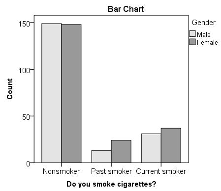
The "clusters" in a clustered bar chart are determined by the row variable (in this case, the smoking categories). The color of the bars is determined by the column variable (in this case, gender). The height of each bar represents the total number of observations in that particular combination of categories.

This type of chart emphasizes the differences within the categories of the row variable. Notice how within each smoking category, the heights of the bars (i.e., the number of males and females) are very similar. That is, there are an approximately equal number of male and female nonsmokers; approximately equal number of male and female past smokers; approximately equal number of male and female current smokers. If there were an association between gender and smoking, we would expect these counts to differ between groups in some way.

Running the Test

• Open the Crosstabs dialog ( Analyze > Descriptive Statistics > Crosstabs ).
• Select Smoking as the row variable, and Gender as the column variable.
• Click Statistics . Check Chi-square , then click Continue .
• (Optional) Check the box for Display clustered bar charts .

The first table is the Case Processing summary, which tells us the number of valid cases used for analysis. Only cases with nonmissing values for both smoking behavior and gender can be used in the test.

The next tables are the crosstabulation and chi-square test results.

The key result in the Chi-Square Tests table is the Pearson Chi-Square.

• The value of the test statistic is 3.171.
• The footnote for this statistic pertains to the expected cell count assumption (i.e., expected cell counts are all greater than 5): no cells had an expected count less than 5, so this assumption was met.
• Because the test statistic is based on a 3x2 crosstabulation table, the degrees of freedom (df) for the test statistic is $$ df = (R - 1)*(C - 1) = (3 - 1)*(2 - 1) = 2*1 = 2 $$.
• The corresponding p-value of the test statistic is p = 0.205.

Decision and Conclusions

Since the p-value is greater than our chosen significance level ( α = 0.05), we do not reject the null hypothesis. Rather, we conclude that there is not enough evidence to suggest an association between gender and smoking.

Based on the results, we can state the following:

• No association was found between gender and smoking behavior ( Χ 2 (2)> = 3.171, p = 0.205).

Example: Chi-square Test for 2x2 Table

Let's continue the row and column percentage example from the Crosstabs tutorial, which described the relationship between the variables RankUpperUnder (upperclassman/underclassman) and LivesOnCampus (lives on campus/lives off-campus). Recall that the column percentages of the crosstab appeared to indicate that upperclassmen were less likely than underclassmen to live on campus:

• The proportion of underclassmen who live off campus is 34.8%, or 79/227.
• The proportion of underclassmen who live on campus is 65.2%, or 148/227.
• The proportion of upperclassmen who live off campus is 94.4%, or 152/161.
• The proportion of upperclassmen who live on campus is 5.6%, or 9/161.

Suppose that we want to test the association between class rank and living on campus using a Chi-Square Test of Independence (using α = 0.05).

The clustered bar chart from the Crosstabs procedure can act as a complement to the column percentages above. Let's look at the chart produced by the Crosstabs procedure for this example:

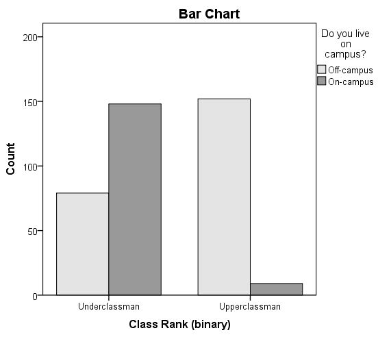
The height of each bar represents the total number of observations in that particular combination of categories. The "clusters" are formed by the row variable (in this case, class rank). This type of chart emphasizes the differences within the underclassmen and upperclassmen groups. Here, the differences in number of students living on campus versus living off-campus is much starker within the class rank groups.

• Select RankUpperUnder as the row variable, and LiveOnCampus as the column variable.
• (Optional) Click Cells . Under Counts, check the boxes for Observed and Expected , and under Residuals, click Unstandardized . Then click Continue .

The first table is the Case Processing summary, which tells us the number of valid cases used for analysis. Only cases with nonmissing values for both class rank and living on campus can be used in the test.

The next table is the crosstabulation. If you elected to check off the boxes for Observed Count, Expected Count, and Unstandardized Residuals, you should see the following table:

With the Expected Count values shown, we can confirm that all cells have an expected value greater than 5.

These numbers can be plugged into the chi-square test statistic formula:

$$ \chi^{2} = \sum_{i=1}^{R}{\sum_{j=1}^{C}{\frac{(o_{ij} - e_{ij})^{2}}{e_{ij}}}} = \frac{(-56.147)^{2}}{135.147} + \frac{(56.147)^{2}}{91.853} + \frac{(56.147)^{2}}{95.853} + \frac{(-56.147)^{2}}{65.147} = 138.926 $$

We can confirm this computation with the results in the Chi-Square Tests table:

The row of interest here is Pearson Chi-Square and its footnote.

• The value of the test statistic is 138.926.
• Because the crosstabulation is a 2x2 table, the degrees of freedom (df) for the test statistic is $$ df = (R - 1)*(C - 1) = (2 - 1)*(2 - 1) = 1 $$.
• The corresponding p-value of the test statistic is so small that it is cut off from display. Instead of writing "p = 0.000", we instead write the mathematically correct statement p < 0.001.

Since the p-value is less than our chosen significance level α = 0.05, we can reject the null hypothesis, and conclude that there is an association between class rank and whether or not students live on-campus.

• There was a significant association between class rank and living on campus ( Χ 2 (1) = 138.9, p < .001).
• << Previous: Analyzing Data
• Next: Pearson Correlation >>
• Last Updated: May 10, 2024 1:32 PM
• URL: https://libguides.library.kent.edu/SPSS

Street Address

Mailing address, quick links.

• How Are We Doing?
• Student Jobs

Information

• Accessibility
• Emergency Information
• For Our Alumni
• For the Media
• Jobs & Employment
• Life at KSU
• Privacy Statement
• Technology Support
• Website Feedback

• school Campus Bookshelves
• menu_book Bookshelves
• perm_media Learning Objects
• login Login
• how_to_reg Request Instructor Account
• hub Instructor Commons

Margin Size

• Download Page (PDF)
• Download Full Book (PDF)
• Periodic Table
• Physics Constants
• Scientific Calculator
• Reference & Cite
• Tools expand_more
• Readability

selected template will load here

This action is not available.

9.4: Probability and Chi-Square Analysis

• Last updated
• Save as PDF
• Page ID 24809

• City Tech CUNY

\( \newcommand{\vecs}[1]{\overset { \scriptstyle \rightharpoonup} {\mathbf{#1}} } \)

\( \newcommand{\vecd}[1]{\overset{-\!-\!\rightharpoonup}{\vphantom{a}\smash {#1}}} \)

\( \newcommand{\id}{\mathrm{id}}\) \( \newcommand{\Span}{\mathrm{span}}\)

( \newcommand{\kernel}{\mathrm{null}\,}\) \( \newcommand{\range}{\mathrm{range}\,}\)

\( \newcommand{\RealPart}{\mathrm{Re}}\) \( \newcommand{\ImaginaryPart}{\mathrm{Im}}\)

\( \newcommand{\Argument}{\mathrm{Arg}}\) \( \newcommand{\norm}[1]{\| #1 \|}\)

\( \newcommand{\inner}[2]{\langle #1, #2 \rangle}\)

\( \newcommand{\Span}{\mathrm{span}}\)

\( \newcommand{\id}{\mathrm{id}}\)

\( \newcommand{\kernel}{\mathrm{null}\,}\)

\( \newcommand{\range}{\mathrm{range}\,}\)

\( \newcommand{\RealPart}{\mathrm{Re}}\)

\( \newcommand{\ImaginaryPart}{\mathrm{Im}}\)

\( \newcommand{\Argument}{\mathrm{Arg}}\)

\( \newcommand{\norm}[1]{\| #1 \|}\)

\( \newcommand{\Span}{\mathrm{span}}\) \( \newcommand{\AA}{\unicode[.8,0]{x212B}}\)

\( \newcommand{\vectorA}[1]{\vec{#1}}      % arrow\)

\( \newcommand{\vectorAt}[1]{\vec{\text{#1}}}      % arrow\)

\( \newcommand{\vectorB}[1]{\overset { \scriptstyle \rightharpoonup} {\mathbf{#1}} } \)

\( \newcommand{\vectorC}[1]{\textbf{#1}} \)

\( \newcommand{\vectorD}[1]{\overrightarrow{#1}} \)

\( \newcommand{\vectorDt}[1]{\overrightarrow{\text{#1}}} \)

\( \newcommand{\vectE}[1]{\overset{-\!-\!\rightharpoonup}{\vphantom{a}\smash{\mathbf {#1}}}} \)

Mendel’s Observations

Probability: Past Punnett Squares

Punnett Squares are convenient for predicting the outcome of monohybrid or dihybrid crosses. The expectation of two heterozygous parents is 3:1 in a single trait cross or 9:3:3:1 in a two-trait cross. Performing a three or four trait cross becomes very messy. In these instances, it is better to follow the rules of probability. Probability is the chance that an event will occur expressed as a fraction or percentage. In the case of a monohybrid cross, 3:1 ratio means that there is a \(\frac{3}{4}\) (0.75) chance of the dominant phenotype with a \(\frac{1}{4}\) (0.25) chance of a recessive phenotype.

A single die has a 1 in 6 chance of being a specific value. In this case, there is a \(\frac{1}{6}\) probability of rolling a 3. It is understood that rolling a second die simultaneously is not influenced by the first and is therefore independent. This second die also has a \(\frac{1}{6}\) chance of being a 3.

We can understand these rules of probability by applying them to the dihybrid cross and realizing we come to the same outcome as the 2 monohybrid Punnett Squares as with the single dihybrid Punnett Square.

This forked line method of calculating probability of offspring with various genotypes and phenotypes can be scaled and applied to more characteristics.

The Chi-Square Test

The χ 2 statistic is used in genetics to illustrate if there are deviations from the expected outcomes of the alleles in a population. The general assumption of any statistical test is that there are no significant deviations between the measured results and the predicted ones. This lack of deviation is called the null hypothesis ( H 0 ). X 2 statistic uses a distribution table to compare results against at varying levels of probabilities or critical values . If the X 2 value is greater than the value at a specific probability, then the null hypothesis has been rejected and a significant deviation from predicted values was observed. Using Mendel’s laws, we can count phenotypes after a cross to compare against those predicted by probabilities (or a Punnett Square).

In order to use the table, one must determine the stringency of the test. The lower the p-value, the more stringent the statistics. Degrees of Freedom ( DF ) are also calculated to determine which value on the table to use. Degrees of Freedom is the number of classes or categories there are in the observations minus 1. DF=n-1

In the example of corn kernel color and texture, there are 4 classes: Purple & Smooth, Purple & Wrinkled, Yellow & Smooth, Yellow & Wrinkled. Therefore, DF = 4 – 1 = 3 and choosing p < 0.05 to be the threshold for significance (rejection of the null hypothesis), the X 2 must be greater than 7.82 in order to be significantly deviating from what is expected. With this dihybrid cross example, we expect a ratio of 9:3:3:1 in phenotypes where 1/16th of the population are recessive for both texture and color while \(\frac{9}{16}\) of the population display both color and texture as the dominant. \(\frac{3}{16}\) will be dominant for one phenotype while recessive for the other and the remaining \(\frac{3}{16}\) will be the opposite combination.

With this in mind, we can predict or have expected outcomes using these ratios. Taking a total count of 200 events in a population, 9/16(200)=112.5 and so forth. Formally, the χ 2 value is generated by summing all combinations of:

\[\frac{(Observed-Expected)^2}{Expected}\]

Chi-Square Test: Is This Coin Fair or Weighted? (Activity)

• Everyone in the class should flip a coin 2x and record the result (assumes class is 24).
• 50% of 48 results should be 24.
• 24 heads and 24 tails are already written in the “Expected” column.
• As a class, compile the results in the “Observed” column (total of 48 coin flips).
• In the last column, subtract the expected heads from the observed heads and square it, then divide by the number of expected heads.
• In the last column, subtract the expected tails from the observed tails and square it, then divide by the number of expected tails.
• Add the values together from the last column to generate the X 2 value.
• There are 2 classes or categories (head or tail), so DF = 2 – 1 = 1.
• Were the coin flips fair (not significantly deviating from 50:50)?

Let’s say that the coin tosses yielded 26 Heads and 22 Tails. Can we assume that the coin was unfair? If we toss a coin an odd number of times (eg. 51), then we would expect that the results would yield 25.5 (50%) Heads and 25.5 (50%) Tails. But this isn’t a possibility. This is when the X 2 test is important as it delineates whether 26:25 or 30:21 etc. are within the probability for a fair coin.

Chi-Square Test of Kernel Coloration and Texture in an F 2 Population (Activity)

• From the counts, one can assume which phenotypes are dominant and recessive.
• Fill in the “Observed” category with the appropriate counts.
• Fill in the “Expected Ratio” with either 9/16, 3/16 or 1/16.
• The total number of the counted event was 200, so multiply the “Expected Ratio” x 200 to generate the “Expected Number” fields.
• Calculate the \(\frac{(Observed-Expected)^2}{Expected}\) for each phenotype combination
• Add all \(\frac{(Observed-Expected)^2}{Expected}\) values together to generate the X 2 value and compare with the value on the table where DF=3.
• What would it mean if the Null Hypothesis was rejected? Can you explain a case in which we have observed values that are significantly altered from what is expected?

LEARN STATISTICS EASILY

Learn Data Analysis Now!

How to Report Chi-Square Test Results in APA Style: A Step-By-Step Guide

In this article, we guide you through how to report Chi-Square Test results, including essential components like the Chi-Square statistic (χ²), degrees of freedom (df), p-value, and Effect Size , aligning with established guidelines for clarity and reproducibility.

Introduction

The Chi-Square Test of Independence is a cornerstone in the field of statistical analysis when researchers aim to examine associations between categorical variables. For instance, in healthcare research, it could be employed to determine whether smoking status is independent of lung cancer incidence within a particular demographic. This statistical technique can decipher the intricacies of frequencies or proportions across different categories, thereby providing robust conclusions on the presence or absence of significant associations.

Conforming to the American Psychological Association (APA) guidelines for statistical reporting not only bolsters the credibility of your findings but also facilitates comprehension among a diversified audience, which may include scholars, healthcare professionals, and policy-makers. Adherence to the APA style is imperative for ensuring that the statistical rigor and the nuances of the Chi-Square Test are communicated effectively and unequivocally.

• The Chi-Square Test evaluates relationships between categorical variables.
• Reporting the Chi-Square, degrees of freedom, p-value, and effect size enhances scientific rigor.
• A p-value under the significance level (generally 0.01 or 0.05) signifies statistical significance.
• For tables larger than 2×2, use adjusted residuals; 5% thresholds are -1.96 and +1.96.
• Cramer’s V and Phi measure effect size and direction.

Ad description. Lorem ipsum dolor sit amet, consectetur adipiscing elit.

Guide to Reporting Chi-Square Test Results

1. state the chi-square test purpose.

Before you delve into the specifics of the Chi-Square Test, clearly outline the research question you aim to answer. The research question will guide your analysis, and it generally revolves around investigating how certain categorical variables might be related to one another.

Once you have a well-framed research question, you must state your hypothesis clearly . The hypothesis will predict what you expect to find in your study. The researcher needs to have a clear understanding of both the null and alternative hypotheses. These hypotheses function as the backbone of the statistical analysis, providing the framework for evaluating the data.

2. Report Sample Size and Characteristics

The sample size is pivotal for the reliability of your results. Indicate how many subjects or items were part of your study and describe the method used for sample size determination.

Offer any relevant demographic information, such as age, gender, socioeconomic status, or other categorical variables that could impact the results. Providing these details will enhance the clarity and comprehensibility of your report.

3. Present Observed Frequencies

For each category or class under investigation, present the observed frequencies . These are the actual counts of subjects or items in each category collected through your research.

The expected frequencies are what you would anticipate if the null hypothesis is true, suggesting no association between the variables. If you prefer, you can also present these expected frequencies in your report to provide additional context for interpretation.

4. Report the Chi-Square Statistic and Degrees of Freedom

Clearly state the Chi-Square value that you calculated during the test. This is often denoted as χ² . It is the test statistic that you’ll compare to a critical value to decide whether to reject the null hypothesis.

In statistical parlance, degrees of freedom refer to the number of values in a study that are free to vary. When reporting your Chi-Square Test results, it is vital to mention the degrees of freedom, typically denoted as “ df .”

5. Indicate the p-value

The p-value is a critical component in statistical hypothesis testing, representing the probability that the observed data would occur if the null hypothesis were true. It quantifies the evidence against the null hypothesis.

Values below 0.05 are commonly considered indicators of statistical significance. This suggests that there is less than a 5% probability of observing a test statistic at least as extreme as the one observed, assuming that the null hypothesis is true. It implies that the association between the variables under study is unlikely to have occurred by random chance alone.

6. Report Effect Size

While a statistically significant p-value can inform you of an association between variables, it does not indicate the strength or magnitude of the relationship. This is where effect size comes into play. Effect size measures such as Cramer’s V or Phi coefficient offer a quantifiable method to determine how strong the association is.

Cramer’s V and Phi coefficient are the most commonly used effect size measures in Chi-Square Tests. Cramer’s V is beneficial for tables larger than 2×2, whereas Phi is generally used for 2×2 tables. Both are derived from the Chi-Square statistic and help compare results across different studies or datasets.

Effect sizes are generally categorized as small (0.1), medium (0.3), or large (0.5). These categories help the audience in making practical interpretations of the study findings.

7. Interpret the Results

Based on the Chi-Square statistic, degrees of freedom, p-value, and effect size, you need to synthesize all this data into coherent and clear conclusions. Here, you must state whether your results support the null hypothesis or suggest that it should be rejected.

Interpreting the results also involves detailing the real-world relevance or practical implications of the findings. For instance, if a Chi-Square Test in a medical study finds a significant association between a particular treatment and patient recovery rates, the practical implication could be that the treatment is effective and should be considered in clinical guidelines.

8. Additional Information

When working with contingency tables larger than 2×2, analyzing the adjusted residuals for each combination of categories between the two nominal qualitative variables becomes necessary. Suppose the significance level is set at 5%. In that case, adjusted residuals with values less than -1.96 or greater than +1.96 indicate an association in the analyzed combination. Similarly, at a 1% significance level, adjusted residuals with values less than -2.576 or greater than +2.576 indicate an association.

Charts , graphs , or tables can be included as supplementary material to represent the statistical data visually. This helps the reader grasp the details and implications of the study more effectively.

Vaccine Efficacy in Two Age Groups

Suppose a study aims to assess whether a new vaccine is equally effective across different age groups: those aged 18-40 and those aged 41-60. A sample of 200 people is randomly chosen, half from each age group. After administering the vaccine, it is observed whether or not the individuals contracted the disease within a specified timeframe.

Observed Frequencies

• Contracted Disease: 12
• Did Not Contract Disease: 88
• Contracted Disease: 28
• Did Not Contract Disease: 72

Expected Frequencies

If there were no association between age group and vaccine efficacy, we would expect an equal proportion of individuals in each group to contract the disease. The expected frequencies would then be:

• Contracted Disease: (12+28)/2 = 20
• Did Not Contract Disease: (88+72)/2 = 80
• Contracted Disease: 20
• Did Not Contract Disease: 80

Chi-Square Test Results

• Chi-Square Statistic (χ²) : 10.8
• Degrees of Freedom (df) : 1
• p-value : 0.001
• Effect Size (Cramer’s V) : 0.23

Interpretation

• Statistical Significance : The p-value being less than 0.05 indicates a statistically significant association between age group and vaccine efficacy.
• Effect Size : The effect size of 0.23, although statistically significant, is on the smaller side, suggesting that while age does have an impact on vaccine efficacy, the practical significance is moderate.
• Practical Implications : Given the significant but moderate association, healthcare providers may consider additional protective measures for the older age group but do not necessarily need to rethink the vaccine’s distribution strategy entirely.

Results Presentation

To evaluate the effectiveness of the vaccine across two different age groups, a Chi-Square Test of Independence was executed. The observed frequencies revealed that among those aged 18-40, 12 contracted the disease, while 88 did not. Conversely, in the 41-60 age group, 28 contracted the disease, and 72 did not. Under the assumption that there was no association between age group and vaccine efficacy, the expected frequencies were calculated to be 20 contracting the disease and 80 not contracting the disease for both age groups. The analysis resulted in a Chi-Square statistic (χ²) of 10.8, with 1 degree of freedom. The associated p-value was 0.001, below the alpha level of 0.05, suggesting a statistically significant association between age group and vaccine efficacy. Additionally, an effect size was calculated using Cramer’s V, which was found to be 0.23. While this effect size is statistically significant, it is moderate in magnitude.

Alternative Results Presentation

To assess the vaccine’s effectiveness across different age demographics, we performed a Chi-Square Test of Independence. In the age bracket of 18-40, observed frequencies indicated that 12 individuals contracted the disease, in contrast to 88 who did not (Expected frequencies: Contracted = 20, Not Contracted = 80). Similarly, for the 41-60 age group, 28 individuals contracted the disease, while 72 did not (Expected frequencies: Contracted = 20, Not Contracted = 80). The Chi-Square Test yielded significant results (χ²(1) = 10.8, p = .001, V = .23). These results imply a statistically significant, albeit moderately sized, association between age group and vaccine efficacy.

Reporting Chi-Square Test results in APA style involves multiple layers of detail. From stating the test’s purpose, presenting sample size, and explaining the observed and expected frequencies to elucidating the Chi-Square statistic, p-value, and effect size, each component serves a unique role in building a compelling narrative around your research findings.

By diligently following this comprehensive guide, you empower your audience to gain a nuanced understanding of your research. This not only enhances the validity and impact of your study but also contributes to the collective scientific endeavor of advancing knowledge.

Recommended Articles

Interested in learning more about statistical analysis and its vital role in scientific research? Explore our blog for more insights and discussions on relevant topics.

Mastering the Chi-Square Test: A Comprehensive Guide

• What is the Difference Between the T-Test vs. Chi-Square Test?
• Understanding the Null Hypothesis in Chi-Square
• Effect Size for Chi-Square Tests: Unveiling its Significance

Understanding the Assumptions for Chi-Square Test of Independence

• Assumptions for Chi-Square Test (Story)
• Chi-Square Calculator: Enhance Your Data Analysis Skills
• Chi Square Test – an overview (Exte rnal Link)

Frequently Asked Questions (FAQs)

The Chi-Square Test of Independence is a statistical method used to evaluate the relationship between two or more categorical variables. It is commonly employed in various research fields to determine if there are significant associations between variables.

Use a Chi-Square Test to examine the relationship between two or more categorical variables. This test is often applied in healthcare, social sciences, and marketing research, among other disciplines.

The p-value represents the probability that the observed data occurred by chance if the null hypothesis is true. A p-value less than 0.05 generally indicates a statistically significant relationship between the variables being studied.

To report the results in APA style, state the purpose, sample size, observed frequencies, Chi-Square statistic, degrees of freedom, p-value, effect size, and interpretation of the findings. Additional information, such as adjusted residuals and graphical representations, may also be included.

Effect size measures like Cramer’s V or Phi coefficient quantify the strength and direction of the relationship between variables. Effect sizes are categorized as small (0.1), medium (0.3), or large (0.5).

Interpret the effect size in terms of its practical implications. For example, a small effect size, although statistically significant, might not be practically important. Conversely, a large effect size would likely have significant real-world implications.

In contingency tables larger than 2×2, adjusted residuals are calculated to identify which specific combinations of categories are driving the observed associations. Thresholds commonly used are -1.96 and +1.96 at a 5% significance level.

Chi-square tests are more reliable with larger sample sizes. For small sample sizes, it is advisable to use an alternative test like Fisher’s Exact Test.

While a t-test is used to compare the means of two groups, a Chi-Square Test is used to examine the relationship between two or more categorical variables. Both tests provide different types of information and are used under other conditions.

Yes, options like the Fisher’s Exact Test for small samples and the Kruskal-Wallis test for ordinal data are available. These are used when the assumptions for a Chi-Square Test cannot be met.

Similar Posts

How to Report Simple Linear Regression Results in APA Style

With this article, you will learn How to Report Simple Linear Regression in APA-style. Ensure accurate, credible research results.

How to Report Results of Multiple Linear Regression in APA Style

Master how to report results of multiple linear regression in APA style, covering coefficients, model fit, and diagnostics.

Uncover the workings, assumptions, and limitations of the Chi-Square Test — a vital tool for analyzing categorical data.

How to Report Results of Simple Binary Logistic Regression

Our guide will help you master how to report results of simple binary logistic regression in APA style, enhancing clarity.

APA Style T-Test Reporting Guide

How to report t-test in APA style? Learn now! Tips, examples, and effect size calculation included. Learn how to report t-test results.

Explore the assumptions and applications of the Chi-Square Test of Independence, a crucial tool for analyzing categorical data in various fields.

Leave a Reply Cancel reply

Your email address will not be published. Required fields are marked *

Save my name, email, and website in this browser for the next time I comment.

If you're seeing this message, it means we're having trouble loading external resources on our website.

If you're behind a web filter, please make sure that the domains *.kastatic.org and *.kasandbox.org are unblocked.

To log in and use all the features of Khan Academy, please enable JavaScript in your browser.

AP®︎/College Statistics

Course: ap®︎/college statistics   >   unit 12.

• Introduction to the chi-square test for homogeneity
• Chi-square test for association (independence)
• Expected counts in chi-squared tests with two-way tables
• Test statistic and P-value in chi-square tests with two-way tables

Making conclusions in chi-square tests for two-way tables

• (Choice A)   This is convincing evidence that color and type of car are not independent. A This is convincing evidence that color and type of car are not independent.
• (Choice B)   We lack evidence to say that color and type of car are not independent. B We lack evidence to say that color and type of car are not independent.
• (Choice C)   This is convincing evidence that the distribution of color differs between trucks and sedans in this population. C This is convincing evidence that the distribution of color differs between trucks and sedans in this population.
• (Choice D)   This isn't enough evidence to say that the distribution of color differs between trucks and sedans in this population. D This isn't enough evidence to say that the distribution of color differs between trucks and sedans in this population.
• (Choice E)   Buying certain types of cars causes people to be more likely to choose certain colors. E Buying certain types of cars causes people to be more likely to choose certain colors.

Statistics Made Easy

How to Interpret Chi-Square Test Results in SPSS

A Chi-Square Test of Independence is used to determine whether or not there is a significant association between two categorical variables.

The following example shows how to interpret the results of a Chi-Square test of Independence in SPSS.

Example: How to Interpret Chi-Square Test of Independence Results in SPSS

Suppose we want to know whether or not gender is associated with political party preference.

We take a simple random sample of 50 voters and survey them on their political party preference.

The following screenshot shows how to enter this data into SPSS:

In the new window that appears, drag Gender  into the Rows panel, then drag Party into the Columns panel:

Next, click the Cells button. Then check the boxes next to Observed and Expected :

Then click Continue .

Next, click the Statistics button. Then check the box next to Chi-square :

Then click OK .

Case Processing Summary

This table displays the number of valid observations and missing observations in the dataset.

We can see that there are 50 valid observations and 0 missing observations.

Crosstabulation

This table displays a crosstab of the total number of individuals by gender and political party preference, including the observed count for each group and the expected count.

Refer to this article for an explanation of how to calculate expected counts in a Chi-Square test.

Chi-Square Tests

This table shows the results of the Chi-Square Test of Independence.

The Chi-Square test statistic is 1.118 and the corresponding two-sided p-value is  .572 .

Recall the hypotheses used for a Chi-Square Test of Independence:

• H 0 : The two variables are independent.
• H A : The two variables are not independent, i.e. they are associated.

In this particular example, our null hypothesis is that gender and political party preference are independent.

Since the p-value ( .572 ) of the test is not less than 0.05 , we fail to reject the null hypothesis.

Thus, we do not have sufficient evidence to say that there is an association between gender and political party preference.

Additional Resources

The following tutorials explain how to perform other common tasks in SPSS:

How to Perform a One Sample t-test in SPSS How to Perform a Two Sample t-test in SPSS How to Create a Frequency Table in SPSS

Featured Posts

Hey there. My name is Zach Bobbitt. I have a Masters of Science degree in Applied Statistics and I’ve worked on machine learning algorithms for professional businesses in both healthcare and retail. I’m passionate about statistics, machine learning, and data visualization and I created Statology to be a resource for both students and teachers alike.  My goal with this site is to help you learn statistics through using simple terms, plenty of real-world examples, and helpful illustrations.

Leave a Reply Cancel reply

Your email address will not be published. Required fields are marked *

Join the Statology Community

Sign up to receive Statology's exclusive study resource: 100 practice problems with step-by-step solutions. Plus, get our latest insights, tutorials, and data analysis tips straight to your inbox!

By subscribing you accept Statology's Privacy Policy.

Chi Square Test

Ai generator.

The chi-square test, a cornerstone of statistical analysis, is utilized to examine the independence of two categorical variables, offering a method to assess observed versus expected frequencies in categorical data. This test extends beyond basic algebra and rational numbers , involving computations with square and square roots , which are integral in determining the chi-square statistic. Unlike dealing with integers or continuous rational and irrational numbers directly, this test quantifies how much observed counts deviate from expected counts in categorical data, rooted in the realm of probability and discrete mathematics . Additionally, while it diverges from the least squares method used for continuous data regression, both share a common goal of minimizing deviation to optimize fit between observed and expected models. In statistics , understanding and applying the chi-square test provides crucial insights into data relationships, crucial for robust analytical conclusions in research and real-world applications.

What is Chi Square Test?

Chi-square distribution.

The chi-square distribution is a fundamental probability distribution in statistics, widely used in hypothesis testing and confidence interval estimation for variance. It arises primarily when summing the squares of independent, standard normal variables, and is characterized by its degrees of freedom, which influence its shape. As the degrees of freedom increase, the distribution becomes more symmetric and approaches a normal distribution. This distribution is crucial in constructing the chi-square test for independence and goodness-of-fit tests, helping to determine whether observed frequencies significantly deviate from expected frequencies under a given hypothesis. It is also integral to the analysis of variance (ANOVA) and other statistical procedures that assess the variability among group means.

Finding P-Value

Step 1: understand the p-value.

The p-value represents the probability of observing a test statistic as extreme as, or more extreme than, the value calculated from the sample data, under the null hypothesis. A low p-value (typically less than 0.05) suggests that the observed data is inconsistent with the null hypothesis, leading to its rejection.

Step 2: Calculate the Test Statistic

Depending on the statistical test being used (like t-test, chi-square test, ANOVA, etc.), first calculate the appropriate test statistic based on your data. This involves different formulas depending on the test and the data structure.

Step 3: Determine the Distribution

Identify the distribution that the test statistic follows under the null hypothesis. For example, the test statistic in a chi-square test follows a chi-square distribution, while a t-test statistic follows a t-distribution.

Step 4: Find the P-Value

Use the distribution identified in Step 3 to find the probability of obtaining a test statistic as extreme as the one you calculated. This can be done using statistical software, tables, or online calculators. You will compare your test statistic to the critical values from the distribution, calculating the area under the curve that lies beyond the test statistic.

Step 5: Interpret the P-Value

• If the p-value is less than the chosen significance level (usually 0.05) , reject the null hypothesis, suggesting that the effect observed in the data is statistically significant.
• If the p-value is greater than the significance level , you do not have enough evidence to reject the null hypothesis, and it is assumed that any observed differences could be due to chance.

Practical Example

For a simpler illustration, suppose you’re conducting a two-tailed t-test with a t-statistic of 2.3, and you’re using a significance level of 0.05. You would:

• Identify that the t-statistic follows a t-distribution with degrees of freedom dependent on your sample size.
• Using a t-distribution table or software, find the probability that a t-value is at least as extreme as ±2.3.
• Sum the probabilities of obtaining a t-value of 2.3 or higher and -2.3 or lower. This sum is your p-value.

Properties of Chi-Square

1. non-negativity.

• The chi-square statistic is always non-negative. This property arises because it is computed as the sum of the squares of standardized differences between observed and expected frequencies.

2. Degrees of Freedom

• The shape and scale of the chi-square distribution are primarily determined by its degrees of freedom, which in turn depend on the number of categories or variables involved in the analysis. The degrees of freedom for a chi-square test are generally calculated as (𝑟−1)(𝑐−1) for an 𝑟×𝑐 contingency table.

3. Distribution Shape

• The chi-square distribution is skewed to the right, especially with fewer degrees of freedom. As the degrees of freedom increase, the distribution becomes more symmetric and starts to resemble a normal distribution.

4. Additivity

• The chi-square distributions are additive. This means that if two independent chi-square variables are added together, their sum also follows a chi-square distribution, with degrees of freedom equal to the sum of their individual degrees of freedom.

5. Dependency on Sample Size

• The chi-square statistic is sensitive to sample size. Larger sample sizes tend to give more reliable estimates of the chi-square statistic, reducing the influence of sampling variability. This property emphasizes the need for adequate sample sizes in experiments intending to use chi-square tests for valid inference.

Chi-Square Formula

Components of the Formula:

• χ ² is the chi-square statistic.
• 𝑂ᵢ​ represents the observed frequency for each category.
• 𝐸ᵢ​ represents the expected frequency for each category, based on the hypothesis being tested.
• The summation (∑) is taken over all categories involved in the test.

Chi-Square Test of Independence

The Chi-Square Test of Independence assesses whether two categorical variables are independent, meaning whether the distribution of one variable differs depending on the value of the other variable.

Assumptions

Before conducting the test, certain assumptions must be met:

• Sample Size : All expected frequencies should be at least 1, and no more than 20% of expected frequencies are less than 5.
• Independence : Observations must be independent of each other, typically achieved by random sampling.
• Data Level : Both variables should be categorical (nominal or ordinal).

Example of Categorical Data

Breakdown of the table.

• Rows : Represent different categories of pet ownership (Owns a Pet, Does Not Own a Pet).
• Columns : Represent preferences for types of pet food (Organic, Non-Organic).
• Cells : Show the frequency of respondents in each combination of categories (e.g., 120 people own a pet and prefer organic pet food).

Below is the representation of a chi-square distribution table with three probability levels (commonly used significance levels: 0.05, 0.01, and 0.001) for degrees of freedom up to 50. The degrees of freedom (DF) for a chi-square test in a contingency table are calculated as (r-1)(c-1), where r is the number of rows and c is the number of columns. This table is vital for determining critical values when testing hypotheses involving categorical data.

This table provides critical values for various degrees of freedom and significance levels, which can be used to determine the likelihood of observing a chi-square statistic at least as extreme as the test statistic calculated from your data, under the assumption that the null hypothesis is true.

Example of Chi-Square Test for Independence

The Chi-square test for independence is a statistical test commonly used to determine if there is a significant relationship between two categorical variables in a population. Let’s go through a detailed example to understand how to apply this test.

Imagine a researcher wants to investigate whether gender (male or female) affects the choice of a major (science or humanities) among university students.

Data Collection

The researcher surveys a sample of 300 students and compiles the data into the following contingency table:

• Null Hypothesis (H₀): There is no relationship between gender and choice of major.
• Alternative Hypothesis (H₁): There is a relationship between gender and choice of major.

1. Calculate Expected Counts:

• Under the null hypothesis, if there’s no relationship between gender and major, the expected count for each cell of the table is calculated by the formula:

Eᵢⱼ ​= (Row Total×Column Total)​/Total Observations

For the ‘Male & Science’ cell:

𝐸ₘₐₗₑ, ₛ꜀ᵢₑₙ꜀ₑ = (150×130)/300 = 65

Repeat this for each cell.

Compute Chi-Square Statistic

The chi-square statistic is calculated using:

χ ² = ∑( O − E )²​/E

Where 𝑂 is the observed frequency, and 𝐸 is the expected frequency. For each cell:

χ ² = 65(70−65)²​+85(80−85)²​+65(60−65)²​+85(90−85) ​ = 1.615

Determine Significance

With 1 degree of freedom (df = (rows – 1)/ times (columns – 1)), check the critical value from the chi-square distribution table at the desired significance level (e.g., 0.05). If 𝜒² calculated is greater than the critical value from the table, reject the null hypothesis.

What does the Chi-Square value indicate?

The Chi-Square value indicates how much the observed frequencies deviate from the expected frequencies under the null hypothesis of independence. A higher Chi-Square value suggests a greater deviation, which may lead to the rejection of the null hypothesis if the value exceeds the critical value from the Chi-Square distribution table for the given degrees of freedom and significance level.

How do you interpret the results of a Chi-Square Test?

To interpret the results of a Chi-Square Test, compare the calculated Chi-Square statistic to the critical value from the Chi-Square distribution table at your chosen significance level (commonly 0.05 or 0.01). If the calculated value is greater than the critical value, reject the null hypothesis, suggesting a significant association between the variables. If it is less, fail to reject the null hypothesis, indicating no significant association.

What are the limitations of the Chi-Square Test?

The Chi-Square Test assumes that the data are from a random sample, observations are independent, and expected frequencies are sufficiently large, typically at least 5 in each cell of the table. When these conditions are not met, the test results may not be valid. Additionally, the test does not provide information about the direction or strength of the association, only its existence.

Text prompt

• Instructive
• Professional

10 Examples of Public speaking

20 Examples of Gas lighting

User Preferences

Content preview.

Arcu felis bibendum ut tristique et egestas quis:

• Ut enim ad minim veniam, quis nostrud exercitation ullamco laboris
• Duis aute irure dolor in reprehenderit in voluptate
• Excepteur sint occaecat cupidatat non proident

Keyboard Shortcuts

Minitab quick guide.

Minitab ®

Access Minitab Web , using Google Chrome  .

Click on the section to view the Minitab procedures.

After saving the Minitab File to your computer or cloud location, you must first open Minitab .

• To open a Minitab project (.mpx file): File > Open > Project
• To open a data file (.mtw, .csv or .xlsx): File > Open > Worksheet

Descriptive, graphical

• Bar Chart : Graph > Bar Chart > Counts of unique values > One Variable
• Pie Chart : Graph > Pie Chart > Counts of unique values > Select Options > Under Label Slices With choose Percent

Descriptive, numerical

• Frequency Tables : Stat > Tables > Tally Individual Variables

Inference (one proportion)

Hypothesis Test

• With raw data : Stat > Basic Statistics > 1 Proportion > Select variable > Check Perform hypothesis test and enter null value > Select Options tab > Choose correct alternative > Under method , choose Normal approximation
• With summarized data : Stat > Basic Statistics > 1 Proportion > Choose Summarized data from the dropdown menu > Enter data > Check Perform hypothesis test and enter null value > Select Options tab > Choose correct alternative > Under method, choose Normal approximation

Confidence Interval

• With raw data : Stat > Basic Statistics > 1 Proportion > Select variable > Select Options tab > Enter correct confidence level, make sure the alternative is set as not-equal, and choose Normal approximation method
• Histogram : Graph > Histogram > Simple
• Dotplot : Graph > Dotplot > One Y, Simple
• Boxplot : Graph > Boxplot > One Y, Simple
• Mean, Std. Dev., 5-number Summary, etc .: Stat > Basic Statistics > Display Descriptive Statistics > Select Statistics tab to choose exactly what you want to display

Inference (one mean)

• With raw data : Stat > Basic Statistics > 1-Sample t > Select variable > Check Perform hypothesis test and enter null value > Select Options tab > Choose the correct alternative
• With summarized data : Stat > Basic Statistics > 1-Sample t > Select Summarized data from the dropdown menu > Enter data (n, x-bar, s) > Check Perform hypothesis test and enter null value > Select Options tab > Choose correct alternative
• With raw data : Stat > Basic Statistics > 1-Sample t > Select variable > Select Options tab > Enter correct confidence level and make sure the alternative is set as not-equal
• With summarized data : Stat > Basic Statistics > 1-Sample t > Select Summarized data from the dropdown menu > Enter data (n, x-bar, s) > Select Options tab > Enter correct confidence level and make sure the alternative is set as not-equal
• Side-by-side Histograms : Graph > Histogram > Under One Y Variable , select Groups Displayed Separately > Enter the categorical variable under Group Variables > Choose In separate panels of one graph under Display Groups
• Side-by-side Dotplots : Graph > Dotplot > One Y Variable , Groups Displayed on the Scale
• Side-by-side Boxplots : Graph > Boxplot > One Y, With Categorical Variables
• Mean, Std. Dev., 5-number Summary, etc .: Stat > Basic Statistics > Display Descriptive Statistics > Select variables (enter the categorical variable under By variables ) > Select Statistics tab to choose exactly what you want to display

Inference (independent samples)

• With raw data : Stat > Basic Statistics > 2-Sample t > Select variables (response/quantitative as Samples and explanatory/categorical as Sample IDs ) > Select Options tab > Choose correct alternative
• With summarized data : Stat > Basic Statistics > 2-Sample t > Select Summarized data from the dropdown menu > Enter data > Select Options tab > Choose correct alternative
• Same as above, choose confidence level and make sure the alternative is set as not-equal

Inference (paired difference)

• Stat > Basic Statistics > Paired t > Enter correct columns in Sample 1 and Sample 2 boxes > Select Options tab > Choose correct alternative
• Scatterplot : Graph > Scatterplot > Simple > Enter the response variable under Y variables and the explanatory variable under X variables
• Fitted Line Plot : Stat > Regression > Fitted Line Plot > Enter the response variable under Response (y) and the explanatory variable under Predictor (x)
• Correlation : Stat > Basic Statistics > Correlation > Select Graphs tab > Click Statistics to display on plot and select Correlations
• Correlation : Stat > Basic Statistics > Correlation > Select Graphs tab > Click Statistics to display on plot and select Correlations and p-values
• Regression Line : Stat > Regression > Regression > Fit Regression Model > Enter the response variable under Responses and the explanatory variable under Continuous predictors > Select Results tab > Click Display of results and select Basic tables ( Note : if you want the confidence interval for the population slope, change “display of results” to “expanded table.” With the expanded table, you will get a lot of information on the output that you will not understand.)
• Side-by-side Bar Charts with raw data : Graph > Bar Chart > Counts of unique values > Multiple Variables
• Side-by-side Bar Charts with a two-way table : Graph > Bar Chart > Summarized Data in a Table > Under Two-Way Table choose Clustered or Stacked > Enter the columns that contain the data under Y-variables and enter the column that contains your row labels under Row labels
• Two-way Table : Stat > Tables > Cross Tabulation and Chi-square

Inference (difference in proportions)

• Using a dataset : Stat > Basic Statistics > 2 Proportions > Select variables (enter response variable as Samples and explanatory variable as Sample IDs ) > Select Options tab > Choose correct alternative
• Using a summary table : Stat > Basic Statistics > 2 Proportions > Select Summarized data from the dropdown menu > Enter data > Select Options tab > Choose correct alternative
• Same as above, choose confidence level and make sure the alternative is set as not equal

Inference (Chi-squared test of association)

• Stat > Tables > Chi-Square Test for Association > Choose correct data option (raw or summarized) > Select variables > Select Statistics tab to choose the statistics you want to display
• Fit multiple regression model : Stat > Regression > Regression > Fit Regression Model > Enter the response variable under Responses , the quantitative explanatory variables under Continuous predictors , and any categorical explanatory variables under Categorical predictors > Select Results tab > Click Display of results and select Basic tables ( Note : if you want the confidence intervals for the coefficients, change display of results to expanded table . You will get a lot of information on the output that you will not understand.)
• Make a prediction or prediction interval using a fitted model : Stat > Regression > Regression > Predict > Enter values for each explanatory variable