hypothesis for correlation

Sciencing_Icons_Science SCIENCE

Sciencing_icons_biology biology, sciencing_icons_cells cells, sciencing_icons_molecular molecular, sciencing_icons_microorganisms microorganisms, sciencing_icons_genetics genetics, sciencing_icons_human body human body, sciencing_icons_ecology ecology, sciencing_icons_chemistry chemistry, sciencing_icons_atomic & molecular structure atomic & molecular structure, sciencing_icons_bonds bonds, sciencing_icons_reactions reactions, sciencing_icons_stoichiometry stoichiometry, sciencing_icons_solutions solutions, sciencing_icons_acids & bases acids & bases, sciencing_icons_thermodynamics thermodynamics, sciencing_icons_organic chemistry organic chemistry, sciencing_icons_physics physics, sciencing_icons_fundamentals-physics fundamentals, sciencing_icons_electronics electronics, sciencing_icons_waves waves, sciencing_icons_energy energy, sciencing_icons_fluid fluid, sciencing_icons_astronomy astronomy, sciencing_icons_geology geology, sciencing_icons_fundamentals-geology fundamentals, sciencing_icons_minerals & rocks minerals & rocks, sciencing_icons_earth scructure earth structure, sciencing_icons_fossils fossils, sciencing_icons_natural disasters natural disasters, sciencing_icons_nature nature, sciencing_icons_ecosystems ecosystems, sciencing_icons_environment environment, sciencing_icons_insects insects, sciencing_icons_plants & mushrooms plants & mushrooms, sciencing_icons_animals animals, sciencing_icons_math math, sciencing_icons_arithmetic arithmetic, sciencing_icons_addition & subtraction addition & subtraction, sciencing_icons_multiplication & division multiplication & division, sciencing_icons_decimals decimals, sciencing_icons_fractions fractions, sciencing_icons_conversions conversions, sciencing_icons_algebra algebra, sciencing_icons_working with units working with units, sciencing_icons_equations & expressions equations & expressions, sciencing_icons_ratios & proportions ratios & proportions, sciencing_icons_inequalities inequalities, sciencing_icons_exponents & logarithms exponents & logarithms, sciencing_icons_factorization factorization, sciencing_icons_functions functions, sciencing_icons_linear equations linear equations, sciencing_icons_graphs graphs, sciencing_icons_quadratics quadratics, sciencing_icons_polynomials polynomials, sciencing_icons_geometry geometry, sciencing_icons_fundamentals-geometry fundamentals, sciencing_icons_cartesian cartesian, sciencing_icons_circles circles, sciencing_icons_solids solids, sciencing_icons_trigonometry trigonometry, sciencing_icons_probability-statistics probability & statistics, sciencing_icons_mean-median-mode mean/median/mode, sciencing_icons_independent-dependent variables independent/dependent variables, sciencing_icons_deviation deviation, sciencing_icons_correlation correlation, sciencing_icons_sampling sampling, sciencing_icons_distributions distributions, sciencing_icons_probability probability, sciencing_icons_calculus calculus, sciencing_icons_differentiation-integration differentiation/integration, sciencing_icons_application application, sciencing_icons_projects projects, sciencing_icons_news news.

• Share Tweet Email Print
• Home ⋅
• Math ⋅
• Probability & Statistics ⋅
• Distributions

How to Write a Hypothesis for Correlation

How to Calculate a P-Value

A hypothesis is a testable statement about how something works in the natural world. While some hypotheses predict a causal relationship between two variables, other hypotheses predict a correlation between them. According to the Research Methods Knowledge Base, a correlation is a single number that describes the relationship between two variables. If you do not predict a causal relationship or cannot measure one objectively, state clearly in your hypothesis that you are merely predicting a correlation.

Research the topic in depth before forming a hypothesis. Without adequate knowledge about the subject matter, you will not be able to decide whether to write a hypothesis for correlation or causation. Read the findings of similar experiments before writing your own hypothesis.

Identify the independent variable and dependent variable. Your hypothesis will be concerned with what happens to the dependent variable when a change is made in the independent variable. In a correlation, the two variables undergo changes at the same time in a significant number of cases. However, this does not mean that the change in the independent variable causes the change in the dependent variable.

Construct an experiment to test your hypothesis. In a correlative experiment, you must be able to measure the exact relationship between two variables. This means you will need to find out how often a change occurs in both variables in terms of a specific percentage.

Establish the requirements of the experiment with regard to statistical significance. Instruct readers exactly how often the variables must correlate to reach a high enough level of statistical significance. This number will vary considerably depending on the field. In a highly technical scientific study, for instance, the variables may need to correlate 98 percent of the time; but in a sociological study, 90 percent correlation may suffice. Look at other studies in your particular field to determine the requirements for statistical significance.

State the null hypothesis. The null hypothesis gives an exact value that implies there is no correlation between the two variables. If the results show a percentage equal to or lower than the value of the null hypothesis, then the variables are not proven to correlate.

Record and summarize the results of your experiment. State whether or not the experiment met the minimum requirements of your hypothesis in terms of both percentage and significance.

Related Articles

How to determine the sample size in a quantitative..., how to calculate a two-tailed test, how to interpret a student's t-test results, how to know if something is significant using spss, quantitative vs. qualitative data and laboratory testing, similarities of univariate & multivariate statistical..., what is the meaning of sample size, distinguishing between descriptive & causal studies, how to calculate cv values, how to determine your practice clep score, what are the different types of correlations, how to calculate p-hat, how to calculate percentage error, how to calculate percent relative range, how to calculate a sample size population, how to calculate bias, how to calculate the percentage of another number, how to find y value for the slope of a line, advantages & disadvantages of finding variance.

• University of New England; Steps in Hypothesis Testing for Correlation; 2000
• Research Methods Knowledge Base; Correlation; William M.K. Trochim; 2006
• Science Buddies; Hypothesis

About the Author

Brian Gabriel has been a writer and blogger since 2009, contributing to various online publications. He earned his Bachelor of Arts in history from Whitworth University.

Photo Credits

Thinkstock/Comstock/Getty Images

Find Your Next Great Science Fair Project! GO

• Flashes Safe Seven
• FlashLine Login
• Faculty & Staff Phone Directory
• Emeriti or Retiree
• All Departments
• Maps & Directions

• Building Guide
• Departments
• Directions & Parking
• Faculty & Staff
• Give to University Libraries
• Library Instructional Spaces
• Mission & Vision
• Newsletters
• Circulation
• Course Reserves / Core Textbooks
• Equipment for Checkout
• Interlibrary Loan
• Library Instruction
• Library Tutorials
• My Library Account
• Open Access Kent State
• Research Support Services
• Statistical Consulting
• Student Multimedia Studio
• Citation Tools
• Databases A-to-Z
• Databases By Subject
• Digital Collections
• Discovery@Kent State
• Government Information
• Journal Finder
• Library Guides
• Connect from Off-Campus
• Library Workshops
• Subject Librarians Directory
• Suggestions/Feedback
• Writing Commons
• Academic Integrity
• Jobs for Students
• International Students
• Meet with a Librarian
• Study Spaces
• University Libraries Student Scholarship
• Affordable Course Materials
• Copyright Services
• Selection Manager
• Suggest a Purchase

Library Locations at the Kent Campus

• Architecture Library
• Fashion Library
• Map Library
• Performing Arts Library
• Special Collections and Archives

Regional Campus Libraries

• East Liverpool
• College of Podiatric Medicine

• Kent State University
• SPSS Tutorials

Pearson Correlation

Spss tutorials: pearson correlation.

• The SPSS Environment
• The Data View Window
• Using SPSS Syntax
• Data Creation in SPSS
• Importing Data into SPSS
• Variable Types
• Date-Time Variables in SPSS
• Defining Variables
• Creating a Codebook
• Computing Variables
• Recoding Variables
• Recoding String Variables (Automatic Recode)
• Weighting Cases
• rank transform converts a set of data values by ordering them from smallest to largest, and then assigning a rank to each value. In SPSS, the Rank Cases procedure can be used to compute the rank transform of a variable." href="https://libguides.library.kent.edu/SPSS/RankCases" style="" >Rank Cases
• Sorting Data
• Grouping Data
• Descriptive Stats for One Numeric Variable (Explore)
• Descriptive Stats for One Numeric Variable (Frequencies)
• Descriptive Stats for Many Numeric Variables (Descriptives)
• Descriptive Stats by Group (Compare Means)
• Frequency Tables
• Working with "Check All That Apply" Survey Data (Multiple Response Sets)
• Chi-Square Test of Independence
• One Sample t Test
• Paired Samples t Test
• Independent Samples t Test
• One-Way ANOVA
• How to Cite the Tutorials

Sample Data Files

Our tutorials reference a dataset called "sample" in many examples. If you'd like to download the sample dataset to work through the examples, choose one of the files below:

• Data definitions (*.pdf)
• Data - Comma delimited (*.csv)
• Data - Tab delimited (*.txt)
• Data - Excel format (*.xlsx)
• Data - SAS format (*.sas7bdat)
• Data - SPSS format (*.sav)
• SPSS Syntax (*.sps) Syntax to add variable labels, value labels, set variable types, and compute several recoded variables used in later tutorials.
• SAS Syntax (*.sas) Syntax to read the CSV-format sample data and set variable labels and formats/value labels.

The bivariate Pearson Correlation produces a sample correlation coefficient, r , which measures the strength and direction of linear relationships between pairs of continuous variables. By extension, the Pearson Correlation evaluates whether there is statistical evidence for a linear relationship among the same pairs of variables in the population, represented by a population correlation coefficient, ρ (“rho”). The Pearson Correlation is a parametric measure.

This measure is also known as:

• Pearson’s correlation
• Pearson product-moment correlation (PPMC)

Common Uses

The bivariate Pearson Correlation is commonly used to measure the following:

• Correlations among pairs of variables
• Correlations within and between sets of variables

The bivariate Pearson correlation indicates the following:

• Whether a statistically significant linear relationship exists between two continuous variables
• The strength of a linear relationship (i.e., how close the relationship is to being a perfectly straight line)
• The direction of a linear relationship (increasing or decreasing)

Note: The bivariate Pearson Correlation cannot address non-linear relationships or relationships among categorical variables. If you wish to understand relationships that involve categorical variables and/or non-linear relationships, you will need to choose another measure of association.

Note: The bivariate Pearson Correlation only reveals associations among continuous variables. The bivariate Pearson Correlation does not provide any inferences about causation, no matter how large the correlation coefficient is.

Data Requirements

To use Pearson correlation, your data must meet the following requirements:

• Two or more continuous variables (i.e., interval or ratio level)
• Cases must have non-missing values on both variables
• Linear relationship between the variables
• the values for all variables across cases are unrelated
• for any case, the value for any variable cannot influence the value of any variable for other cases
• no case can influence another case on any variable
• The biviariate Pearson correlation coefficient and corresponding significance test are not robust when independence is violated.
• Each pair of variables is bivariately normally distributed
• Each pair of variables is bivariately normally distributed at all levels of the other variable(s)
• This assumption ensures that the variables are linearly related; violations of this assumption may indicate that non-linear relationships among variables exist. Linearity can be assessed visually using a scatterplot of the data.
• Random sample of data from the population
• No outliers

The null hypothesis ( H 0 ) and alternative hypothesis ( H 1 ) of the significance test for correlation can be expressed in the following ways, depending on whether a one-tailed or two-tailed test is requested:

Two-tailed significance test:

H 0 : ρ  = 0 ("the population correlation coefficient is 0; there is no association") H 1 : ρ ≠ 0 ("the population correlation coefficient is not 0; a nonzero correlation could exist")

One-tailed significance test:

H 0 : ρ  = 0 ("the population correlation coefficient is 0; there is no association") H 1 : ρ   > 0 ("the population correlation coefficient is greater than 0; a positive correlation could exist")      OR H 1 : ρ   < 0 ("the population correlation coefficient is less than 0; a negative correlation could exist")

where ρ is the population correlation coefficient.

Test Statistic

The sample correlation coefficient between two variables x and y is denoted r or r xy , and can be computed as: $$ r_{xy} = \frac{\mathrm{cov}(x,y)}{\sqrt{\mathrm{var}(x)} \dot{} \sqrt{\mathrm{var}(y)}} $$

where cov( x , y ) is the sample covariance of x and y ; var( x ) is the sample variance of x ; and var( y ) is the sample variance of y .

Correlation can take on any value in the range [-1, 1]. The sign of the correlation coefficient indicates the direction of the relationship, while the magnitude of the correlation (how close it is to -1 or +1) indicates the strength of the relationship.

•  -1 : perfectly negative linear relationship
•   0 : no relationship
• +1  : perfectly positive linear relationship

The strength can be assessed by these general guidelines [1] (which may vary by discipline):

• .1 < | r | < .3 … small / weak correlation
• .3 < | r | < .5 … medium / moderate correlation
• .5 < | r | ……… large / strong correlation

Note: The direction and strength of a correlation are two distinct properties. The scatterplots below [2] show correlations that are r = +0.90, r = 0.00, and r = -0.90, respectively. The strength of the nonzero correlations are the same: 0.90. But the direction of the correlations is different: a negative correlation corresponds to a decreasing relationship, while and a positive correlation corresponds to an increasing relationship. 

Note that the r = 0.00 correlation has no discernable increasing or decreasing linear pattern in this particular graph. However, keep in mind that Pearson correlation is only capable of detecting linear associations, so it is possible to have a pair of variables with a strong nonlinear relationship and a small Pearson correlation coefficient. It is good practice to create scatterplots of your variables to corroborate your correlation coefficients.

[1]  Cohen, J. (1988). Statistical power analysis for the behavioral sciences (2nd ed.). Hillsdale, NJ: Lawrence Erlbaum Associates.

[2]  Scatterplots created in R using ggplot2 , ggthemes::theme_tufte() , and MASS::mvrnorm() .

Data Set-Up

Your dataset should include two or more continuous numeric variables, each defined as scale, which will be used in the analysis.

Each row in the dataset should represent one unique subject, person, or unit. All of the measurements taken on that person or unit should appear in that row. If measurements for one subject appear on multiple rows -- for example, if you have measurements from different time points on separate rows -- you should reshape your data to "wide" format before you compute the correlations.

Run a Bivariate Pearson Correlation

To run a bivariate Pearson Correlation in SPSS, click  Analyze > Correlate > Bivariate .

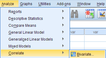
The Bivariate Correlations window opens, where you will specify the variables to be used in the analysis. All of the variables in your dataset appear in the list on the left side. To select variables for the analysis, select the variables in the list on the left and click the blue arrow button to move them to the right, in the Variables field.

A Variables : The variables to be used in the bivariate Pearson Correlation. You must select at least two continuous variables, but may select more than two. The test will produce correlation coefficients for each pair of variables in this list.

B Correlation Coefficients: There are multiple types of correlation coefficients. By default, Pearson is selected. Selecting Pearson will produce the test statistics for a bivariate Pearson Correlation.

C Test of Significance:  Click Two-tailed or One-tailed , depending on your desired significance test. SPSS uses a two-tailed test by default.

D Flag significant correlations: Checking this option will include asterisks (**) next to statistically significant correlations in the output. By default, SPSS marks statistical significance at the alpha = 0.05 and alpha = 0.01 levels, but not at the alpha = 0.001 level (which is treated as alpha = 0.01)

E Options : Clicking Options will open a window where you can specify which Statistics to include (i.e., Means and standard deviations , Cross-product deviations and covariances ) and how to address Missing Values (i.e., Exclude cases pairwise or Exclude cases listwise ). Note that the pairwise/listwise setting does not affect your computations if you are only entering two variable, but can make a very large difference if you are entering three or more variables into the correlation procedure.

Example: Understanding the linear association between weight and height

Problem statement.

Perhaps you would like to test whether there is a statistically significant linear relationship between two continuous variables, weight and height (and by extension, infer whether the association is significant in the population). You can use a bivariate Pearson Correlation to test whether there is a statistically significant linear relationship between height and weight, and to determine the strength and direction of the association.

Before the Test

In the sample data, we will use two variables: “Height” and “Weight.” The variable “Height” is a continuous measure of height in inches and exhibits a range of values from 55.00 to 84.41 ( Analyze > Descriptive Statistics > Descriptives ). The variable “Weight” is a continuous measure of weight in pounds and exhibits a range of values from 101.71 to 350.07.

Before we look at the Pearson correlations, we should look at the scatterplots of our variables to get an idea of what to expect. In particular, we need to determine if it's reasonable to assume that our variables have linear relationships. Click Graphs > Legacy Dialogs > Scatter/Dot . In the Scatter/Dot window, click Simple Scatter , then click Define . Move variable Height to the X Axis box, and move variable Weight to the Y Axis box. When finished, click OK .

To add a linear fit like the one depicted, double-click on the plot in the Output Viewer to open the Chart Editor. Click Elements > Fit Line at Total . In the Properties window, make sure the Fit Method is set to Linear , then click Apply . (Notice that adding the linear regression trend line will also add the R-squared value in the margin of the plot. If we take the square root of this number, it should match the value of the Pearson correlation we obtain.)

From the scatterplot, we can see that as height increases, weight also tends to increase. There does appear to be some linear relationship.

Running the Test

To run the bivariate Pearson Correlation, click  Analyze > Correlate > Bivariate . Select the variables Height and Weight and move them to the Variables box. In the Correlation Coefficients area, select Pearson . In the Test of Significance area, select your desired significance test, two-tailed or one-tailed. We will select a two-tailed significance test in this example. Check the box next to Flag significant correlations .

Click OK to run the bivariate Pearson Correlation. Output for the analysis will display in the Output Viewer.

The results will display the correlations in a table, labeled Correlations .

A Correlation of Height with itself (r=1), and the number of nonmissing observations for height (n=408).

B Correlation of height and weight (r=0.513), based on n=354 observations with pairwise nonmissing values.

C Correlation of height and weight (r=0.513), based on n=354 observations with pairwise nonmissing values.

D Correlation of weight with itself (r=1), and the number of nonmissing observations for weight (n=376).

The important cells we want to look at are either B or C. (Cells B and C are identical, because they include information about the same pair of variables.) Cells B and C contain the correlation coefficient for the correlation between height and weight, its p-value, and the number of complete pairwise observations that the calculation was based on.

The correlations in the main diagonal (cells A and D) are all equal to 1. This is because a variable is always perfectly correlated with itself. Notice, however, that the sample sizes are different in cell A ( n =408) versus cell D ( n =376). This is because of missing data -- there are more missing observations for variable Weight than there are for variable Height.

If you have opted to flag significant correlations, SPSS will mark a 0.05 significance level with one asterisk (*) and a 0.01 significance level with two asterisks (0.01). In cell B (repeated in cell C), we can see that the Pearson correlation coefficient for height and weight is .513, which is significant ( p < .001 for a two-tailed test), based on 354 complete observations (i.e., cases with nonmissing values for both height and weight).

Decision and Conclusions

Based on the results, we can state the following:

• Weight and height have a statistically significant linear relationship ( r =.513, p < .001).
• The direction of the relationship is positive (i.e., height and weight are positively correlated), meaning that these variables tend to increase together (i.e., greater height is associated with greater weight).
• The magnitude, or strength, of the association is approximately moderate (.3 < | r | < .5).
• << Previous: Chi-Square Test of Independence
• Next: One Sample t Test >>
• Last Updated: Apr 10, 2024 4:50 PM
• URL: https://libguides.library.kent.edu/SPSS

Street Address

Mailing address, quick links.

• How Are We Doing?
• Student Jobs

Information

• Accessibility
• Emergency Information
• For Our Alumni
• For the Media
• Jobs & Employment
• Life at KSU
• Privacy Statement
• Technology Support
• Website Feedback

User Preferences

Content preview.

Arcu felis bibendum ut tristique et egestas quis:

• Ut enim ad minim veniam, quis nostrud exercitation ullamco laboris
• Duis aute irure dolor in reprehenderit in voluptate
• Excepteur sint occaecat cupidatat non proident

Keyboard Shortcuts

5.3 - inferences for correlations.

Let us consider testing the null hypothesis that there is zero correlation between two variables \(X_{j}\) and \(X_{k}\). Mathematically we write this as shown below:

\(H_0\colon \rho_{jk}=0\) against \(H_a\colon \rho_{jk} \ne 0 \)

Recall that the correlation is estimated by sample correlation \(r_{jk}\) given in the expression below:

\(r_{jk} = \dfrac{s_{jk}}{\sqrt{s^2_js^2_k}}\)

Here we have the sample covariance between the two variables divided by the square root of the product of the individual variances.

We shall assume that the pair of variables \(X_{j}\)and \(X_{k}\) are independently sampled from a bivariate normal distribution throughout this discussion; that is:

\(\left(\begin{array}{c}X_{1j}\\X_{1k} \end{array}\right)\), \(\left(\begin{array}{c}X_{2j}\\X_{2k} \end{array}\right)\), \(\dots\), \(\left(\begin{array}{c}X_{nj}\\X_{nk} \end{array}\right)\)

are independently sampled from a bivariate normal distribution.

To test the null hypothesis, we form the test statistic, t  as below

\(t = r_{jk}\sqrt{\frac{n-2}{1-r^2_{jk}}}\)  \(\dot{\sim}\)  \( t_{n-2}\)

Under the null hypothesis, \(H_{o}\), this test statistic will be approximately distributed as t with n - 2 degrees of freedom.

Note! This approximation holds for larger samples. We will reject the null hypothesis, \(H_{o}\), at level \(α\) if the absolute value of the test statistic, t , is greater than the critical value from the t -table with n - 2 degrees of freedom; that is if:

\(|t| > t_{n-2, \alpha/2}\)

To illustrate these concepts let's return to our example dataset, the Wechsler Adult Intelligence Scale.

Example 5-5: Wechsler Adult Intelligence Scale Section  

•   Example

This data was analyzed using the SAS program in our last lesson, (Multivariate Normal Distribution), which yielded the computer output below.

Download the:

Dataset:  wechsler.csv

SAS program: wechsler.sas

SAS Output: wechsler.lst

Find the Total Variance of the Wechsler Adult Intelligence Scale Data

To find the correlation matrix:

• Open the ‘wechsler’ data set in a new worksheet
• Stat > Basic Statistics > Correlation
• Highlight and select ‘info’, ‘sim’, ‘arith’, and ‘pict’ to move them into the variables window
• Select ‘ OK ’. The matrix of correlations, along with scatterplots, is displayed in the results area

Recall that these are data on n = 37 subjects taking the Wechsler Adult Intelligence Test. This test was broken up into four components:

• Information
• Similarities
• Picture Completion

Looking at the computer output we have summarized the correlations among variables in the table below:

For example, the correlation between Similarities and Information is 0.77153.

Let's consider testing the null hypothesis that there is no correlation between Information and Similarities. This would be written mathematically as shown below:

\(H_0\colon \rho_{12}=0\)

We can then substitute values into the formula to compute the test statistic using the values from this example:

\begin{align} t &= r_{jk}\sqrt{\frac{n-2}{1-r^2_{jk}}}\\[10pt] &= 0.77153 \sqrt{\frac{37-2}{1-0.77153^2}}\\[10pt] &= 7.175 \end{align}

Looking at our t -table for 35 degrees of freedom and an \(\alpha\) level of .005, we get a critical value of \(t _ { ( d f , 1 - \alpha / 2 ) } = t _ { 35,0.9975 } = 3.030\). Therefore, we are going to look at the critical value under 0.0025 in the table (since 35 does not appear to use the closest df that does not exceed 35 which is 30) and in this case it is 3.030, meaning that \(t _ { ( d f , 1 - \alpha / 2 ) } = t _ { 35,0.9975 } = 3.030\) is close to 3.030.

Note! Some text tables provide the right tail probability (the graph at the top will have the area in the right tail shaded in) while other texts will provide a table with the cumulative probability - the graph will be shaded into the left. The concept is the same. For example, if the alpha was 0.01 then using the first text you would look under 0.005, and in the second text look under 0.995.

 Because

\(7.175 > 3.030 = t_{35, 0.9975}\),

we can reject the null hypothesis that Information and Similarities scores are uncorrelated at the \(\alpha\) < 0.005 level.

Our conclusion is that Similarity scores increase with increasing Information scores ( t = 7.175; d.f . = 35; p < 0.0001). You will note here that we are not simply concluding that the results are significant. When drawing conclusions it is never adequate to simply state that the results are significant. In all cases, you should seek to describe what the results tell you about this data. In this case, because we rejected the null hypothesis we can conclude that the correlation is not equal to zero.  Furthermore, because the actual sample correlation is greater than zero and our p-value is so small, we can conclude that there is a positive association between the two variables. Hence, our conclusion is that Similarity scores tend to increase with increasing values of Information scores.

You will also note that the conclusion includes information from the test. You should always back up your findings with the appropriate evidence: the test statistic, degrees of freedom (if appropriate), and p -value. Here the appropriate evidence is given by the test statistic t = 7.175; the degrees of freedom for the test, 35, and the p -value, less than 0.0001 as indicated by the computer printout. The p -value appears below each correlation coefficient in the SAS output.

Confidence Interval for \(p_{jk}\) Section  

Once we conclude that there is a positive or negative correlation between two variables the next thing we might want to do is compute a confidence interval for the correlation. This confidence interval will give us a range of reasonable values for the correlation itself. The sample correlation, because it is bounded between -1 and 1 is typically not normally distributed or even approximately so. If the population correlation is near zero, the distribution of sample correlations may be approximately bell-shaped in distribution around zero. However, if the population correlation is near +1 or -1, the distribution of sample correlations will be skewed. For example, if \(p_{jk}= .9\), the distribution of sample correlations will be more concentrated near .9.  Because they cannot exceed 1, they have more room to spread out to the left of .9, which causes a left-skewed shape. To adjust for this asymmetry or the skewness of distribution, we apply a transformation of the correlation coefficients. In particular, we are going to apply Fisher's transformation which is given in the expression below in Step 1 of our procedure for computing confidence intervals for the correlation coefficient.

\(z_{jk}=\frac{1}{2}\log\dfrac{1+r_{jk}}{1-r_{jk}}\)

Here we have one-half of the natural log of 1 plus the correlation, divided by one minus the correlation.

Note! In this course, whenever log is mentioned, unless specified otherwise, log stands for the natural log.

For large samples, this transform correlation coefficient z is going to be approximately normally distributed with the mean equal to the same transformation of the population correlation, as shown below, and a variance of 1 over the sample size minus 3.

\(z_{jk}\) \(\dot{\sim}\) \(N\left(\dfrac{1}{2}\log\dfrac{1+\rho_{jk}}{1-\rho_{jk}}, \dfrac{1}{n-3}\right)\)

Compute a (1 - \(\alpha\)) x 100% confidence interval for the Fisher transform of the population correlation.

\(\dfrac{1}{2}\log \dfrac{1+\rho_{jk}}{1-\rho_{jk}}\)

That is one-half log of 1 plus the correlation divided by 1 minus the correlation. In other words, this confidence interval is given by the expression below:

\(\left(\underset{Z_l}{\underbrace{Z_{jk}-\frac{Z_{\alpha/2}}{\sqrt{n-3}}}}, \underset{Z_U}{\underbrace{Z_{jk}+\frac{Z_{\alpha/2}}{\sqrt{n-3}}}}\right)\)

Here we take the value of Fisher's transform Z , plus and minus the critical value from the z table, divided by the square root of n - 3. The lower bound we will call the \(Z_{1}\) and the upper bound we will call the \(Z_{u}\).

Back transform the confidence values to obtain the desired confidence interval for \(\rho_{jk}\) This is given in the expression below:

\(\left(\dfrac{e^{2Z_l}-1}{e^{2Z_l}+1},\dfrac{e^{2Z_U}-1}{e^{2Z_U}+1}\right)\)

The first term we see is a function of the lower bound, the \(Z_{1}\). The second term is a function of the upper bound or \(Z_{u}\).

Let's return to the Wechsler Adult Intelligence Data to see how these procedures are carried out.

Example 5-6: Wechsler Adult Intelligence Data Section  

Recall that the sample correlation between Similarities and Information was \(r_{12} = 0.77153\).

Step 1 : Compute the Fisher transform:

\begin{align} Z_{12} &= \frac{1}{2}\log \frac{1+r_{12}}{1-r_{12}}\\[5pt] &= \frac{1}{2}\log\frac{1+0.77153}{1-0.77153}\\[5pt] &= 1.024 \end{align}

You should confirm this value on your own.

Step 2 : Next, compute the 95% confidence interval for the Fisher transform, \(\frac{1}{2}\log \frac{1+\rho_{12}}{1-\rho_{12}}\) :

\begin{align} Z_l &=  Z_{12}-Z_{0.025}/\sqrt{n-3} \\ &= 1.024 - \frac{1.96}{\sqrt{37-3}} \\ &= 0.6880 \end{align}

\begin{align} Z_U &=  Z_{12}+Z_{0.025}/\sqrt{n-3} \\&= 1.024 + \frac{1.96}{\sqrt{37-3}} \\&= 1.3602 \end{align}

In other words, the value 1.024 plus or minus the critical value from the normal table, at \(α/2 = 0.025\), which in this case is 1.96. Divide by the square root of n minus 3. Subtracting the result from 1.024 yields a lower bound of 0.6880. Adding the result to 1.024 yields the upper bound of 1.3602.

Step 3 : Carry out the back-transform to obtain the 95% confidence interval for ρ 12 . This is shown in the expression below:

\(\left(\dfrac{\exp\{2Z_l\}-1}{\exp\{2Z_l\}+1},\dfrac{\exp\{2Z_U\}-1}{\exp\{2Z_U\}+1}\right)\) 

\(\left(\dfrac{\exp\{2 \times 0.6880\}-1}{\exp\{2 \times 0.6880\}+1},\dfrac{\exp\{2\times 1.3602\}-1}{\exp\{2\times 1.3602\}+1}\right)\)

\((0.5967,0.8764)\)

This yields the interval from 0.5967 to 0.8764 .

Conclusion : In this case, we can conclude that we are 95% confident that the interval (0.5967, 0.8764) contains the correlation between Information and Similarities scores.

Module 12: Linear Regression and Correlation

Testing the significance of the correlation coefficient, learning outcomes.

• Calculate and interpret the correlation coefficient

The correlation coefficient,  r , tells us about the strength and direction of the linear relationship between x and y . However, the reliability of the linear model also depends on how many observed data points are in the sample. We need to look at both the value of the correlation coefficient r and the sample size n , together.

We perform a hypothesis test of the “ significance of the correlation coefficient ” to decide whether the linear relationship in the sample data is strong enough to use to model the relationship in the population.

The sample data are used to compute  r , the correlation coefficient for the sample. If we had data for the entire population, we could find the population correlation coefficient. But because we have only have sample data, we cannot calculate the population correlation coefficient. The sample correlation coefficient, r , is our estimate of the unknown population correlation coefficient.

• The symbol for the population correlation coefficient is ρ , the Greek letter “rho.”
• ρ = population correlation coefficient (unknown)
• r = sample correlation coefficient (known; calculated from sample data)

The hypothesis test lets us decide whether the value of the population correlation coefficient ρ is “close to zero” or “significantly different from zero”. We decide this based on the sample correlation coefficient r and the sample size n .

If the test concludes that the correlation coefficient is significantly different from zero, we say that the correlation coefficient is “significant.” Conclusion: There is sufficient evidence to conclude that there is a significant linear relationship between x and y because the correlation coefficient is significantly different from zero. What the conclusion means: There is a significant linear relationship between x and y . We can use the regression line to model the linear relationship between x and y in the population.

If the test concludes that the correlation coefficient is not significantly different from zero (it is close to zero), we say that correlation coefficient is “not significant.”

Conclusion: “There is insufficient evidence to conclude that there is a significant linear relationship between x and y because the correlation coefficient is not significantly different from zero.” What the conclusion means: There is not a significant linear relationship between x and y . Therefore, we CANNOT use the regression line to model a linear relationship between x and y in the population.

• If r is significant and the scatter plot shows a linear trend, the line can be used to predict the value of y for values of x that are within the domain of observed x values.
• If r is not significant OR if the scatter plot does not show a linear trend, the line should not be used for prediction.
• If r is significant and if the scatter plot shows a linear trend, the line may NOT be appropriate or reliable for prediction OUTSIDE the domain of observed x values in the data.

Performing the Hypothesis Test

• Null Hypothesis: H 0 : ρ = 0
• Alternate Hypothesis: H a : ρ ≠ 0

What the Hypotheses Mean in Words

• Null Hypothesis H 0 : The population correlation coefficient IS NOT significantly different from zero. There IS NOT a significant linear relationship(correlation) between x and y in the population.
• Alternate Hypothesis H a : The population correlation coefficient IS significantly DIFFERENT FROM zero. There IS A SIGNIFICANT LINEAR RELATIONSHIP (correlation) between x and y in the population.

Drawing a Conclusion

There are two methods of making the decision. The two methods are equivalent and give the same result.

• Method 1: Using the p -value
• Method 2: Using a table of critical values

In this chapter of this textbook, we will always use a significance level of 5%,  α = 0.05

Using the  p -value method, you could choose any appropriate significance level you want; you are not limited to using α = 0.05. But the table of critical values provided in this textbook assumes that we are using a significance level of 5%, α = 0.05. (If we wanted to use a different significance level than 5% with the critical value method, we would need different tables of critical values that are not provided in this textbook.)

Method 1: Using a p -value to make a decision

To calculate the  p -value using LinRegTTEST:

• On the LinRegTTEST input screen, on the line prompt for β or ρ , highlight “≠ 0”
• The output screen shows the p-value on the line that reads “p =”.
• (Most computer statistical software can calculate the p -value.)

If the p -value is less than the significance level ( α = 0.05)

• Decision: Reject the null hypothesis.
• Conclusion: “There is sufficient evidence to conclude that there is a significant linear relationship between x and y because the correlation coefficient is significantly different from zero.”

If the p -value is NOT less than the significance level ( α = 0.05)

• Decision: DO NOT REJECT the null hypothesis.
• Conclusion: “There is insufficient evidence to conclude that there is a significant linear relationship between x and y because the correlation coefficient is NOT significantly different from zero.”

Calculation Notes:

• You will use technology to calculate the p -value. The following describes the calculations to compute the test statistics and the p -value:
• The p -value is calculated using a t -distribution with n – 2 degrees of freedom.
• The formula for the test statistic is [latex]\displaystyle{t}=\frac{{{r}\sqrt{{{n}-{2}}}}}{\sqrt{{{1}-{r}^{{2}}}}}[/latex]. The value of the test statistic, t , is shown in the computer or calculator output along with the p -value. The test statistic t has the same sign as the correlation coefficient r .
• The p -value is the combined area in both tails.

An alternative way to calculate the  p -value (p) given by LinRegTTest is the command 2*tcdf(abs(t),10^99, n-2) in 2nd DISTR.

Method 2: Using a table of Critical Values to make a decision

The 95% Critical Values of the Sample Correlation Coefficient Table can be used to give you a good idea of whether the computed value of is significant or not. Compare  r to the appropriate critical value in the table. If r is not between the positive and negative critical values, then the correlation coefficient is significant. If r is significant, then you may want to use the line for prediction.

Suppose you computed  r = 0.801 using n = 10 data points. df = n – 2 = 10 – 2 = 8. The critical values associated with df = 8 are -0.632 and + 0.632. If r < negative critical value or r > positive critical value, then r is  significant . Since r = 0.801 and 0.801 > 0.632, r is significant and the line may be used for prediction. If you view this example on a number line, it will help you.

For a given line of best fit, you computed that  r = 0.6501 using n = 12 data points and the critical value is 0.576. Can the line be used for prediction? Why or why not?

If the scatter plot looks linear then, yes, the line can be used for prediction, because  r > the positive critical value.

Suppose you computed  r = –0.624 with 14 data points. df = 14 – 2 = 12. The critical values are –0.532 and 0.532. Since –0.624 < –0.532, r is significant and the line can be used for prediction

For a given line of best fit, you compute that  r = 0.5204 using n = 9 data points, and the critical value is 0.666. Can the line be used for prediction? Why or why not?

No, the line cannot be used for prediction, because  r < the positive critical value.

Suppose you computed  r = 0.776 and n = 6. df = 6 – 2 = 4. The critical values are –0.811 and 0.811. Since –0.811 < 0.776 < 0.811, r is not significant, and the line should not be used for prediction.

–0.811 <  r = 0.776 < 0.811. Therefore, r is not significant.

For a given line of best fit, you compute that  r = –0.7204 using n = 8 data points, and the critical value is = 0.707. Can the line be used for prediction? Why or why not?

Yes, the line can be used for prediction, because  r < the negative critical value.

Suppose you computed the following correlation coefficients. Using the table at the end of the chapter, determine if  r is significant and the line of best fit associated with each r can be used to predict a y value. If it helps, draw a number line.

• r = –0.567 and the sample size, n , is 19. The df = n – 2 = 17. The critical value is –0.456. –0.567 < –0.456 so r is significant.
• r = 0.708 and the sample size, n , is nine. The df = n – 2 = 7. The critical value is 0.666. 0.708 > 0.666 so r is significant.
• r = 0.134 and the sample size, n , is 14. The df = 14 – 2 = 12. The critical value is 0.532. 0.134 is between –0.532 and 0.532 so r is not significant.
• r = 0 and the sample size, n , is five. No matter what the dfs are, r = 0 is between the two critical values so r is not significant.

For a given line of best fit, you compute that  r = 0 using n = 100 data points. Can the line be used for prediction? Why or why not?

No, the line cannot be used for prediction no matter what the sample size is.

Assumptions in Testing the Significance of the Correlation Coefficient

Testing the significance of the correlation coefficient requires that certain assumptions about the data are satisfied. The premise of this test is that the data are a sample of observed points taken from a larger population. We have not examined the entire population because it is not possible or feasible to do so. We are examining the sample to draw a conclusion about whether the linear relationship that we see between x and y in the sample data provides strong enough evidence so that we can conclude that there is a linear relationship between x and y in the population.

The regression line equation that we calculate from the sample data gives the best-fit line for our particular sample. We want to use this best-fit line for the sample as an estimate of the best-fit line for the population. Examining the scatterplot and testing the significance of the correlation coefficient helps us determine if it is appropriate to do this.

The assumptions underlying the test of significance are:

• There is a linear relationship in the population that models the average value of y for varying values of x . In other words, the expected value of y for each particular value lies on a straight line in the population. (We do not know the equation for the line for the population. Our regression line from the sample is our best estimate of this line in the population.)
• The y values for any particular x value are normally distributed about the line. This implies that there are more y values scattered closer to the line than are scattered farther away. Assumption (1) implies that these normal distributions are centered on the line: the means of these normal distributions of y values lie on the line.
• The standard deviations of the population y values about the line are equal for each value of x . In other words, each of these normal distributions of y values has the same shape and spread about the line.
• The residual errors are mutually independent (no pattern).
• The data are produced from a well-designed, random sample or randomized experiment.

The  y values for each x value are normally distributed about the line with the same standard deviation. For each x value, the mean of the y values lies on the regression line. More y values lie near the line than are scattered further away from the line.

Concept Review

Linear regression is a procedure for fitting a straight line of the form [latex]\displaystyle\hat{{y}}={a}+{b}{x}[/latex] to data. The conditions for regression are:

• Linear: In the population, there is a linear relationship that models the average value of y for different values of x .
• Independent: The residuals are assumed to be independent.
• Normal: The y values are distributed normally for any value of x .
• Equal variance: The standard deviation of the y values is equal for each x value.
• Random: The data are produced from a well-designed random sample or randomized experiment.

The slope  b and intercept a of the least-squares line estimate the slope β and intercept α of the population (true) regression line. To estimate the population standard deviation of y , σ , use the standard deviation of the residuals, s .

[latex]\displaystyle{s}=\sqrt{{\frac{{{S}{S}{E}}}{{{n}-{2}}}}}[/latex] The variable ρ (rho) is the population correlation coefficient.

To test the null hypothesis  H 0 : ρ = hypothesized value , use a linear regression t-test. The most common null hypothesis is H 0 : ρ = 0 which indicates there is no linear relationship between x and y in the population.

The TI-83, 83+, 84, 84+ calculator function LinRegTTest can perform this test (STATS TESTS LinRegTTest).

Formula Review

Least Squares Line or Line of Best Fit: [latex]\displaystyle\hat{{y}}={a}+{b}{x}[/latex]

where  a = y -intercept,  b = slope

Standard deviation of the residuals:

[latex]\displaystyle{s}=\sqrt{{\frac{{{S}{S}{E}}}{{{n}-{2}}}}}[/latex]

SSE = sum of squared errors

n = the number of data points

• OpenStax, Statistics, Testing the Significance of the Correlation Coefficient. Provided by : OpenStax. Located at : http://cnx.org/contents/[email protected]:83/Introductory_Statistics . License : CC BY: Attribution
• Introductory Statistics . Authored by : Barbara Illowski, Susan Dean. Provided by : Open Stax. Located at : http://cnx.org/contents/[email protected] . License : CC BY: Attribution . License Terms : Download for free at http://cnx.org/contents/[email protected]

13.2 Testing the Significance of the Correlation Coefficient

The correlation coefficient, r , tells us about the strength and direction of the linear relationship between X 1 and X 2 .

The sample data are used to compute r , the correlation coefficient for the sample. If we had data for the entire population, we could find the population correlation coefficient. But because we have only sample data, we cannot calculate the population correlation coefficient. The sample correlation coefficient, r , is our estimate of the unknown population correlation coefficient.

• ρ = population correlation coefficient (unknown)
• r = sample correlation coefficient (known; calculated from sample data)

The hypothesis test lets us decide whether the value of the population correlation coefficient ρ is "close to zero" or "significantly different from zero". We decide this based on the sample correlation coefficient r and the sample size n .

If the test concludes that the correlation coefficient is significantly different from zero, we say that the correlation coefficient is "significant."

• Conclusion: There is sufficient evidence to conclude that there is a significant linear relationship between X 1 and X 2 because the correlation coefficient is significantly different from zero.
• What the conclusion means: There is a significant linear relationship X 1 and X 2 . If the test concludes that the correlation coefficient is not significantly different from zero (it is close to zero), we say that correlation coefficient is "not significant".

Performing the Hypothesis Test

• Null Hypothesis: H 0 : ρ = 0
• Alternate Hypothesis: H a : ρ ≠ 0
• Null Hypothesis H 0 : The population correlation coefficient IS NOT significantly different from zero. There IS NOT a significant linear relationship (correlation) between X 1 and X 2 in the population.
• Alternate Hypothesis H a : The population correlation coefficient is significantly different from zero. There is a significant linear relationship (correlation) between X 1 and X 2 in the population.

Drawing a Conclusion There are two methods of making the decision concerning the hypothesis. The test statistic to test this hypothesis is:

Where the second formula is an equivalent form of the test statistic, n is the sample size and the degrees of freedom are n-2. This is a t-statistic and operates in the same way as other t tests. Calculate the t-value and compare that with the critical value from the t-table at the appropriate degrees of freedom and the level of confidence you wish to maintain. If the calculated value is in the tail then cannot accept the null hypothesis that there is no linear relationship between these two independent random variables. If the calculated t-value is NOT in the tailed then cannot reject the null hypothesis that there is no linear relationship between the two variables.

A quick shorthand way to test correlations is the relationship between the sample size and the correlation. If:

then this implies that the correlation between the two variables demonstrates that a linear relationship exists and is statistically significant at approximately the 0.05 level of significance. As the formula indicates, there is an inverse relationship between the sample size and the required correlation for significance of a linear relationship. With only 10 observations, the required correlation for significance is 0.6325, for 30 observations the required correlation for significance decreases to 0.3651 and at 100 observations the required level is only 0.2000.

Correlations may be helpful in visualizing the data, but are not appropriately used to "explain" a relationship between two variables. Perhaps no single statistic is more misused than the correlation coefficient. Citing correlations between health conditions and everything from place of residence to eye color have the effect of implying a cause and effect relationship. This simply cannot be accomplished with a correlation coefficient. The correlation coefficient is, of course, innocent of this misinterpretation. It is the duty of the analyst to use a statistic that is designed to test for cause and effect relationships and report only those results if they are intending to make such a claim. The problem is that passing this more rigorous test is difficult so lazy and/or unscrupulous "researchers" fall back on correlations when they cannot make their case legitimately.

As an Amazon Associate we earn from qualifying purchases.

This book may not be used in the training of large language models or otherwise be ingested into large language models or generative AI offerings without OpenStax's permission.

Want to cite, share, or modify this book? This book uses the Creative Commons Attribution License and you must attribute OpenStax.

Access for free at https://openstax.org/books/introductory-business-statistics/pages/1-introduction

• Authors: Alexander Holmes, Barbara Illowsky, Susan Dean
• Publisher/website: OpenStax
• Book title: Introductory Business Statistics
• Publication date: Nov 29, 2017
• Location: Houston, Texas
• Book URL: https://openstax.org/books/introductory-business-statistics/pages/1-introduction
• Section URL: https://openstax.org/books/introductory-business-statistics/pages/13-2-testing-the-significance-of-the-correlation-coefficient

© Jun 23, 2022 OpenStax. Textbook content produced by OpenStax is licensed under a Creative Commons Attribution License . The OpenStax name, OpenStax logo, OpenStax book covers, OpenStax CNX name, and OpenStax CNX logo are not subject to the Creative Commons license and may not be reproduced without the prior and express written consent of Rice University.

Correlation Calculator

Input your values with a space or comma between in the table below

Critical Value

Results shown here

Sample size, n

Sample correlation coefficient, r, standardized sample score.

• school Campus Bookshelves
• menu_book Bookshelves
• perm_media Learning Objects
• login Login
• how_to_reg Request Instructor Account
• hub Instructor Commons
• Download Page (PDF)
• Download Full Book (PDF)
• Periodic Table
• Physics Constants
• Scientific Calculator
• Reference & Cite
• Tools expand_more
• Readability

selected template will load here

This action is not available.

10.1: Testing the Significance of the Correlation Coefficient

• Last updated
• Save as PDF
• Page ID 10998

The correlation coefficient, \(r\), tells us about the strength and direction of the linear relationship between \(x\) and \(y\). However, the reliability of the linear model also depends on how many observed data points are in the sample. We need to look at both the value of the correlation coefficient \(r\) and the sample size \(n\), together. We perform a hypothesis test of the "significance of the correlation coefficient" to decide whether the linear relationship in the sample data is strong enough to use to model the relationship in the population.

The sample data are used to compute \(r\), the correlation coefficient for the sample. If we had data for the entire population, we could find the population correlation coefficient. But because we have only sample data, we cannot calculate the population correlation coefficient. The sample correlation coefficient, \(r\), is our estimate of the unknown population correlation coefficient.

• The symbol for the population correlation coefficient is \(\rho\), the Greek letter "rho."
• \(\rho =\) population correlation coefficient (unknown)
• \(r =\) sample correlation coefficient (known; calculated from sample data)

The hypothesis test lets us decide whether the value of the population correlation coefficient \(\rho\) is "close to zero" or "significantly different from zero". We decide this based on the sample correlation coefficient \(r\) and the sample size \(n\).

If the test concludes that the correlation coefficient is significantly different from zero, we say that the correlation coefficient is "significant."

• Conclusion: There is sufficient evidence to conclude that there is a significant linear relationship between \(x\) and \(y\) because the correlation coefficient is significantly different from zero.
• What the conclusion means: There is a significant linear relationship between \(x\) and \(y\). We can use the regression line to model the linear relationship between \(x\) and \(y\) in the population.

If the test concludes that the correlation coefficient is not significantly different from zero (it is close to zero), we say that correlation coefficient is "not significant".

• Conclusion: "There is insufficient evidence to conclude that there is a significant linear relationship between \(x\) and \(y\) because the correlation coefficient is not significantly different from zero."
• What the conclusion means: There is not a significant linear relationship between \(x\) and \(y\). Therefore, we CANNOT use the regression line to model a linear relationship between \(x\) and \(y\) in the population.
• If \(r\) is significant and the scatter plot shows a linear trend, the line can be used to predict the value of \(y\) for values of \(x\) that are within the domain of observed \(x\) values.
• If \(r\) is not significant OR if the scatter plot does not show a linear trend, the line should not be used for prediction.
• If \(r\) is significant and if the scatter plot shows a linear trend, the line may NOT be appropriate or reliable for prediction OUTSIDE the domain of observed \(x\) values in the data.

PERFORMING THE HYPOTHESIS TEST

• Null Hypothesis: \(H_{0}: \rho = 0\)
• Alternate Hypothesis: \(H_{a}: \rho \neq 0\)

WHAT THE HYPOTHESES MEAN IN WORDS:

• Null Hypothesis \(H_{0}\) : The population correlation coefficient IS NOT significantly different from zero. There IS NOT a significant linear relationship(correlation) between \(x\) and \(y\) in the population.
• Alternate Hypothesis \(H_{a}\) : The population correlation coefficient IS significantly DIFFERENT FROM zero. There IS A SIGNIFICANT LINEAR RELATIONSHIP (correlation) between \(x\) and \(y\) in the population.

DRAWING A CONCLUSION:There are two methods of making the decision. The two methods are equivalent and give the same result.

• Method 1: Using the \(p\text{-value}\)
• Method 2: Using a table of critical values

In this chapter of this textbook, we will always use a significance level of 5%, \(\alpha = 0.05\)

Using the \(p\text{-value}\) method, you could choose any appropriate significance level you want; you are not limited to using \(\alpha = 0.05\). But the table of critical values provided in this textbook assumes that we are using a significance level of 5%, \(\alpha = 0.05\). (If we wanted to use a different significance level than 5% with the critical value method, we would need different tables of critical values that are not provided in this textbook.)

METHOD 1: Using a \(p\text{-value}\) to make a decision

Using the ti83, 83+, 84, 84+ calculator.

To calculate the \(p\text{-value}\) using LinRegTTEST:

On the LinRegTTEST input screen, on the line prompt for \(\beta\) or \(\rho\), highlight "\(\neq 0\)"

The output screen shows the \(p\text{-value}\) on the line that reads "\(p =\)".

(Most computer statistical software can calculate the \(p\text{-value}\).)

If the \(p\text{-value}\) is less than the significance level ( \(\alpha = 0.05\) ):

• Decision: Reject the null hypothesis.
• Conclusion: "There is sufficient evidence to conclude that there is a significant linear relationship between \(x\) and \(y\) because the correlation coefficient is significantly different from zero."

If the \(p\text{-value}\) is NOT less than the significance level ( \(\alpha = 0.05\) )

• Decision: DO NOT REJECT the null hypothesis.
• Conclusion: "There is insufficient evidence to conclude that there is a significant linear relationship between \(x\) and \(y\) because the correlation coefficient is NOT significantly different from zero."

Calculation Notes:

• You will use technology to calculate the \(p\text{-value}\). The following describes the calculations to compute the test statistics and the \(p\text{-value}\):
• The \(p\text{-value}\) is calculated using a \(t\)-distribution with \(n - 2\) degrees of freedom.
• The formula for the test statistic is \(t = \frac{r\sqrt{n-2}}{\sqrt{1-r^{2}}}\). The value of the test statistic, \(t\), is shown in the computer or calculator output along with the \(p\text{-value}\). The test statistic \(t\) has the same sign as the correlation coefficient \(r\).
• The \(p\text{-value}\) is the combined area in both tails.

An alternative way to calculate the \(p\text{-value}\) ( \(p\) ) given by LinRegTTest is the command 2*tcdf(abs(t),10^99, n-2) in 2nd DISTR.

THIRD-EXAM vs FINAL-EXAM EXAMPLE: \(p\text{-value}\) method

• Consider the third exam/final exam example.
• The line of best fit is: \(\hat{y} = -173.51 + 4.83x\) with \(r = 0.6631\) and there are \(n = 11\) data points.
• Can the regression line be used for prediction? Given a third exam score ( \(x\) value), can we use the line to predict the final exam score (predicted \(y\) value)?
• \(H_{0}: \rho = 0\)
• \(H_{a}: \rho \neq 0\)
• \(\alpha = 0.05\)
• The \(p\text{-value}\) is 0.026 (from LinRegTTest on your calculator or from computer software).
• The \(p\text{-value}\), 0.026, is less than the significance level of \(\alpha = 0.05\).
• Decision: Reject the Null Hypothesis \(H_{0}\)
• Conclusion: There is sufficient evidence to conclude that there is a significant linear relationship between the third exam score (\(x\)) and the final exam score (\(y\)) because the correlation coefficient is significantly different from zero.

Because \(r\) is significant and the scatter plot shows a linear trend, the regression line can be used to predict final exam scores.

METHOD 2: Using a table of Critical Values to make a decision

The 95% Critical Values of the Sample Correlation Coefficient Table can be used to give you a good idea of whether the computed value of \(r\) is significant or not . Compare \(r\) to the appropriate critical value in the table. If \(r\) is not between the positive and negative critical values, then the correlation coefficient is significant. If \(r\) is significant, then you may want to use the line for prediction.

Example \(\PageIndex{1}\)

Suppose you computed \(r = 0.801\) using \(n = 10\) data points. \(df = n - 2 = 10 - 2 = 8\). The critical values associated with \(df = 8\) are \(-0.632\) and \(+0.632\). If \(r <\) negative critical value or \(r >\) positive critical value, then \(r\) is significant. Since \(r = 0.801\) and \(0.801 > 0.632\), \(r\) is significant and the line may be used for prediction. If you view this example on a number line, it will help you.

Exercise \(\PageIndex{1}\)

For a given line of best fit, you computed that \(r = 0.6501\) using \(n = 12\) data points and the critical value is 0.576. Can the line be used for prediction? Why or why not?

If the scatter plot looks linear then, yes, the line can be used for prediction, because \(r >\) the positive critical value.

Example \(\PageIndex{2}\)

Suppose you computed \(r = –0.624\) with 14 data points. \(df = 14 – 2 = 12\). The critical values are \(-0.532\) and \(0.532\). Since \(-0.624 < -0.532\), \(r\) is significant and the line can be used for prediction

Exercise \(\PageIndex{2}\)

For a given line of best fit, you compute that \(r = 0.5204\) using \(n = 9\) data points, and the critical value is \(0.666\). Can the line be used for prediction? Why or why not?

No, the line cannot be used for prediction, because \(r <\) the positive critical value.

Example \(\PageIndex{3}\)

Suppose you computed \(r = 0.776\) and \(n = 6\). \(df = 6 - 2 = 4\). The critical values are \(-0.811\) and \(0.811\). Since \(-0.811 < 0.776 < 0.811\), \(r\) is not significant, and the line should not be used for prediction.

Exercise \(\PageIndex{3}\)

For a given line of best fit, you compute that \(r = -0.7204\) using \(n = 8\) data points, and the critical value is \(= 0.707\). Can the line be used for prediction? Why or why not?

Yes, the line can be used for prediction, because \(r <\) the negative critical value.

THIRD-EXAM vs FINAL-EXAM EXAMPLE: critical value method

Consider the third exam/final exam example. The line of best fit is: \(\hat{y} = -173.51 + 4.83x\) with \(r = 0.6631\) and there are \(n = 11\) data points. Can the regression line be used for prediction? Given a third-exam score ( \(x\) value), can we use the line to predict the final exam score (predicted \(y\) value)?

• Use the "95% Critical Value" table for \(r\) with \(df = n - 2 = 11 - 2 = 9\).
• The critical values are \(-0.602\) and \(+0.602\)
• Since \(0.6631 > 0.602\), \(r\) is significant.
• Conclusion:There is sufficient evidence to conclude that there is a significant linear relationship between the third exam score (\(x\)) and the final exam score (\(y\)) because the correlation coefficient is significantly different from zero.

Example \(\PageIndex{4}\)

Suppose you computed the following correlation coefficients. Using the table at the end of the chapter, determine if \(r\) is significant and the line of best fit associated with each r can be used to predict a \(y\) value. If it helps, draw a number line.

• \(r = –0.567\) and the sample size, \(n\), is \(19\). The \(df = n - 2 = 17\). The critical value is \(-0.456\). \(-0.567 < -0.456\) so \(r\) is significant.
• \(r = 0.708\) and the sample size, \(n\), is \(9\). The \(df = n - 2 = 7\). The critical value is \(0.666\). \(0.708 > 0.666\) so \(r\) is significant.
• \(r = 0.134\) and the sample size, \(n\), is \(14\). The \(df = 14 - 2 = 12\). The critical value is \(0.532\). \(0.134\) is between \(-0.532\) and \(0.532\) so \(r\) is not significant.
• \(r = 0\) and the sample size, \(n\), is five. No matter what the \(dfs\) are, \(r = 0\) is between the two critical values so \(r\) is not significant.

Exercise \(\PageIndex{4}\)

For a given line of best fit, you compute that \(r = 0\) using \(n = 100\) data points. Can the line be used for prediction? Why or why not?

No, the line cannot be used for prediction no matter what the sample size is.

Assumptions in Testing the Significance of the Correlation Coefficient

Testing the significance of the correlation coefficient requires that certain assumptions about the data are satisfied. The premise of this test is that the data are a sample of observed points taken from a larger population. We have not examined the entire population because it is not possible or feasible to do so. We are examining the sample to draw a conclusion about whether the linear relationship that we see between \(x\) and \(y\) in the sample data provides strong enough evidence so that we can conclude that there is a linear relationship between \(x\) and \(y\) in the population.

The regression line equation that we calculate from the sample data gives the best-fit line for our particular sample. We want to use this best-fit line for the sample as an estimate of the best-fit line for the population. Examining the scatter plot and testing the significance of the correlation coefficient helps us determine if it is appropriate to do this.

The assumptions underlying the test of significance are:

• There is a linear relationship in the population that models the average value of \(y\) for varying values of \(x\). In other words, the expected value of \(y\) for each particular value lies on a straight line in the population. (We do not know the equation for the line for the population. Our regression line from the sample is our best estimate of this line in the population.)
• The \(y\) values for any particular \(x\) value are normally distributed about the line. This implies that there are more \(y\) values scattered closer to the line than are scattered farther away. Assumption (1) implies that these normal distributions are centered on the line: the means of these normal distributions of \(y\) values lie on the line.
• The standard deviations of the population \(y\) values about the line are equal for each value of \(x\). In other words, each of these normal distributions of \(y\) values has the same shape and spread about the line.
• The residual errors are mutually independent (no pattern).
• The data are produced from a well-designed, random sample or randomized experiment.

Linear regression is a procedure for fitting a straight line of the form \(\hat{y} = a + bx\) to data. The conditions for regression are:

• Linear In the population, there is a linear relationship that models the average value of \(y\) for different values of \(x\).
• Independent The residuals are assumed to be independent.
• Normal The \(y\) values are distributed normally for any value of \(x\).
• Equal variance The standard deviation of the \(y\) values is equal for each \(x\) value.
• Random The data are produced from a well-designed random sample or randomized experiment.

The slope \(b\) and intercept \(a\) of the least-squares line estimate the slope \(\beta\) and intercept \(\alpha\) of the population (true) regression line. To estimate the population standard deviation of \(y\), \(\sigma\), use the standard deviation of the residuals, \(s\). \(s = \sqrt{\frac{SEE}{n-2}}\). The variable \(\rho\) (rho) is the population correlation coefficient. To test the null hypothesis \(H_{0}: \rho =\) hypothesized value , use a linear regression t-test. The most common null hypothesis is \(H_{0}: \rho = 0\) which indicates there is no linear relationship between \(x\) and \(y\) in the population. The TI-83, 83+, 84, 84+ calculator function LinRegTTest can perform this test (STATS TESTS LinRegTTest).

Formula Review

Least Squares Line or Line of Best Fit:

\[\hat{y} = a + bx\]

\[a = y\text{-intercept}\]

\[b = \text{slope}\]

Standard deviation of the residuals:

\[s = \sqrt{\frac{SSE}{n-2}}\]

\[SSE = \text{sum of squared errors}\]

\[n = \text{the number of data points}\]