case study household income

An official website of the United States government

The .gov means it’s official. Federal government websites often end in .gov or .mil. Before sharing sensitive information, make sure you’re on a federal government site.

The site is secure. The https:// ensures that you are connecting to the official website and that any information you provide is encrypted and transmitted securely.

• Publications
• Account settings

Preview improvements coming to the PMC website in October 2024. Learn More or Try it out now .

• Advanced Search
• Journal List
• Springer Nature - PMC COVID-19 Collection

Well-Being and Stability among Low-income Families: A 10-Year Review of Research

Yoshie sano.

1 Department of Human Development, Washington State University Vancouver, 14204 NE Salmon Creek Avenue, Vancouver, WA 98686 USA

Sheila Mammen

2 Department of Resource Economics, University of Massachusetts Amherst, 309 Stockbridge Hall, Amherst, MA 01003 USA

Myah Houghten

3 Child and Family Research Unit, Washington State University Extension, 412 E. Spokane Falls Blvd, Spokane, WA 99202 USA

Scholarship on families in poverty, in the last decade, documented various struggles and challenges faced by low-income families and expanded our understanding of their complicated life circumstances embedded within the contexts of community, culture, and policies. The research articles published in the Journal of Family and Economic Issues during this time, that highlighted poverty, focused primarily on three topic areas: economic security, family life issues, and food security. Overall, findings conclude that family well-being and stability cannot be promoted without the consideration of environmental factors. They depend on the interaction among individual (e.g., increased human capital), family (e.g., positive co-parental relationship), community (e.g., affordable childcare), and policy changes (e.g., realistic welfare-to-work programs). Collectively, the articles have provided a road map for future research directions.

Introduction

Family well-being, essential to the smooth functioning of communities and societies, is hindered when there is high incidence of poverty. Poverty rate in the US hovered around 14% prior to the enactment of the Personal Responsibility and Work Opportunity Reconciliation Act (PROWRA) of 1996 (U.S. Census 2019a ). Following welfare reform, the poverty rate started to decline (to a low of 11.3% in 2000) (U.S. Census 2019a ), although scholars have questioned if PROWRA is the cause of this decline. Uncertainties in the economy, including the 2008 Great Recession, caused the poverty rate to climb again and remain at around 15% until 2014. With the fading effects of the recession, the US poverty rate was at 11.8% in early 2020, right before the current Coronavirus pandemic. One group that is most vulnerable to poverty, however, are female-headed households, who consistently comprise 50% of all households living in poverty. Other vulnerable groups include non-Whites [poverty rate in 2018, Blacks: 22%; Hispanics: 19%; Native Americans: 24%] (Kaiser Family Foundation 2020 ); rural communities [poverty rate in 2018, non-metro: 16%; metro: 13%] (Economic Research Service 2020 ); and children [poverty rate in 2018, 16%; i.e. 1 in every 6 children] (US Census 2019b ).

Family well-being is a multidimensional concept that refers to a family’s subjective sense of overall welfare, taking into account the physical and emotional health of family members as well as their interconnectedness, which in turn results in family stability (a sense of consistency, predictability, and continuity). There are many components that contribute to the well-being of families such as income sufficiency, food security, stable family environment, mental and physical health security, safe housing and communities, employment opportunities, and adequate transportation. These components, taken as a whole, provide the necessary foundation for the well-being of families. For low-income families, in particular, the lack of some or all of these dimensions can be severely detrimental to their well-being since this could lead to poverty. Such a direct link between lack of well-being and poverty can ultimately lead to family instability.

In this paper, we will review select research findings of the past decade published in the Journal of Family and Economic Issues from 2010 to 2019 that have increased our understanding of low-income families living in poverty. Each study employed a unique approach to its particular topic. Some studies utilized large secondary datasets including both metropolitan and non-metropolitan residents while others collected their own data from a smaller sample generated by non-probability sampling. However, all studies focused on low-income families in the United States with the exception of one study that examined poverty-related social policy in Columbia. The 29 papers, 1 while highly diverse, all illustrated the strengths and challenges faced by individuals and families living with limited resources.

Our review was carried out in multiple stages. First, each author independently reviewed the 29 articles, and then the authors qualitatively compared and contrasted the main themes that emerged from these articles. In the last step, the authors identified three specific dimensions of well-being 2 : economic security, family life, and food security. Our objective was not to provide a comprehensive summary of all poverty-related issues addressed in these articles but, rather, to synthesize the research findings along these three dimensions to see how they have contributed to the current knowledge base regarding low-income families and to provide a path for future research in order to improve family well-being and stability.

Families in Poverty: Decade in Review

Economic security among low-income families.

In the last decade, research on the economic security of low-income families has centered around poverty dynamics, the effectiveness of welfare-to-work programs, employment issues, the Earned Income Tax Credit, and banking behavior.

Poverty Dynamics

Mammen et al. ( 2015 ) developed the Economic Well-Being Continuum (EWC) as a comprehensive measure to describe the circumstances of low-income families in eight specific dimensions (child care, employability, food security, health care security, housing security, transportation, reliance of assistance programs, and capabilities) and establish their level of economic functioning (persistently poor, struggling, and getting by). When certain life circumstances and trigger events experienced by low-income mothers, which contributed to their entry into and exit from poverty, were examined with the EWC, the authors found that family health issues and changes in mothers’ intimate relationships acted as significant trigger events that established or altered the economic functioning of the families. We believe that what mitigated families’ hardships was their support networks. Prawitz et al. ( 2013 ) reported on the centrality of locus of control among low-income individuals who expressed less financial distress and more hopefulness when locus of control was more internal to them. When low-income individuals were able to make financial adjustments, however, they had more financial distress, accompanied with more hopefulness, possibly implying that while the current situation may be bleak, their adaptive responses may have fostered hopefulness that things would improve.

Effectiveness of Welfare-to-Work Programs Among Low-Income Families

One of the goals of PRWORA was to enable recipients of Temporary Assistance for Needy Families (TANF) to exit the program and enter the job market. The transition from welfare to work, however, was not as effective when low-income individuals were trained only through labor force attachment (LFA) programs. Kim ( 2010 , 2012 ) found that former TANF recipients were more likely to obtain employment when LFA programs were combined with human capital development (HCD) programs as participation in HCD programs were related to longer employment durations and lower probability of TANF re-entry.

Participants in Welfare-to-Work programs, who succeeded leaving assistance and obtaining employment, disclosed low wages; informal labor market activity; notable levels of unmet needs; and continued government, community, and social support use (Livermore et al. 2011 ). Those with higher earnings and regular nonmonetary help from family and friends were likely to have more needs met; those who had fewer needs met reported lower wages, had more young children, used government support programs (including childcare subsidies), and engaged in informal labor market activity (Davis et al. 2018 ; Grobe et al. 2017 ; Livermore et al. 2011 ).

Employment Issues

An important way to exit poverty and attain economic security is through employment. Unfortunately, many low-income mothers, especially rural low-income mothers, face daunting challenges to remain employed. Son and Bauer ( 2010 ) reported that mothers who were able to remain in the same job did so because they utilized their limited resources and developed strategies to combine work and family life. These strategies included utilizing social support network for childcare and other household activities as well as relying, where possible, on flexibility at work such as non-standard work hours and supportive supervisors.

One way that low-income mothers were more likely to be employed, and especially employed full-time, was if they were provided state childcare subsidy (Davis et al. 2018 ) and the receipt of childcare subsidy was tied to their employment (Grobe et al. 2017 ). High level of job instability (job loss, major reduction in work hours), however, created a greater likelihood of losing the childcare subsidy. While job changes per se was not related to loss of childcare subsidy, parents required the subsidy to remain employed.

The Earned Income Tax Credit (EITC)

The EITC program, initiated in 1975, is the largest federal assistance program targeted towards working poor families in order to supplement their household wages and to offset their Social Security taxes (Mammen et al. 2011 ). Despite the many benefits of the EITC, a substantial portion of working families, especially in rural communities, do not participate in the program. Mammen et al. ( 2011 ) found that, among rural low-income women, the EITC non-participants were more likely to be Hispanic, be less educated, have larger families, perceive their income as being inadequate, live in more rural counties, and possess little understanding of the EITC. Participating rural working mothers, on the other hand, were more likely to be single, food secure, and satisfied with life.

One important element of the EITC program is the frequency with which the tax credit payments are received by the working families: lumpsum, periodic, or monthly. Kramer et al. ( 2019 ) reported that periodic EITC payment recipients experienced significantly lower levels of perceived financial stress. This relationship was partly mediated by less need to borrow money, lower levels of food insecurity, and fewer unpaid bills. Therefore, periodic EITC payments may enhance the positive association between the EITC and financial well-being of families.

Banking Behavior of Low-Income Families

Having a bank account is more likely to enable low-income families to build assets and to offset unexpected financial expenditures. According to the Federal Deposit Insurance Commission (FDIC), among households with incomes less than $30,000, 38% of them were unbanked in 2017 (Federal Deposit Insurance Corporation 2018 ). Grinstein-Weiss et al. ( 2010 ) found that low-income households who did not have a bank account (unbanked) were more likely to be younger, Black, unpartnered, have more children, and have less income. They were also less likely to have attended college and less likely to be employed full-time. Banked participants, however, were more likely to have better saving performance in Individual Development Accounts (IDA) 3 programs and lower risks of dropping out the IDA programs. According to Rao and Malapit ( 2015 ), for female-headed households, having an additional child increased their likelihood to be underbanked or unbanked. Such financial behavior is more prevalent among female-headed households compared to couples or male-headed households, likely due to the opportunity cost of time for women and the intimidation they feel, perhaps, based on their lack of banking sophistication.

Family Life Issues

Family is where individuals seek rest and support, take nutrition, promote good health and, perhaps, most importantly, raise the next generation. In this section we will discuss findings from the last decade on work-family balance, parenting dynamics, and child well-being and poverty.

Work and Family Life

Many rural low-income families face daunting challenges to balance work and family life. Katras et al. ( 2015 ) found low-income families were able to juggle the demands of work and family life if they had access to resources such as informal social support, could manage both work and family time, and were in jobs that supported work and family life. Difficulties regarding availability of resources or inflexibility in employment created problems in work and family life balance (Katras et al. 2015 ). As mentioned previously, low-income mothers relied on informal support for childcare and household tasks. They also depended on sympathetic supervisors who provided flexible work hours (Son and Bauer 2010 ).

Work-family life balance that working mothers try to achieve can be easily sabotaged by housing instability. Kull et al. ( 2016 ) reported that higher residential mobility was associated with changes in employment status and relationships, experiences of intimate partner violence, as well as private-market rentals, substandard housing, and bad neighborhoods.

Parenting Dynamics

In their study of unmarried couples who coparented children, Jamison et al. ( 2017 ) documented that the difficulties of living in poverty, combined with the demands of parenting young children, can create stress and chaos. Parents who were successful in coparenting were those who were able to manage their limited resources well. Jamison et al. concluded that the best way of assisting low-income couples manage day-to-day stress is by providing them with adequate resources as well as information on how to use these resources effectively.

Traditionally, poverty research has focused on low-income mothers. Myers ( 2013 ), however, studied how low-income fathers defined responsible fatherhood. Previous findings on middle-class fathers have emphasized the importance of breadwinning and childcare rearing roles (Schoppe-Sullivan and Fagon 2020 ). Low-income fathers, who did not provide finances or primary care, on the other hand, did not consider responsible fatherhood to include provision for either of these two functions. Instead they defined responsible fatherhood as spending time in non-caregiving activities, voluntarily distancing themselves from a child when it is in the child’s interest to do so, acknowledging paternity in non-legal settings, spending money on presents, engaging in fun activities, attending to special needs, keeping abreast of what is going on in the child’s home, and ensuring that they are not absent from the child’s life (Myers 2013 ).

Child Well-Being and Poverty

The association between poverty and negative child outcomes has been well-established. Children growing up in poverty are more likely to experience negative health outcomes, poor academic performance, higher dropout rates, and behavioral issues compared to children in middle- and upper-income households (Brooks-Gunn and Duncan 1997 ). Focusing on three economic indicators (income, material hardship, and non-liquid assets), Kainz et al. ( 2012 ) found an association among them and variations in 36-month old children’s social and cognitive development. Poverty status, measured by income-to-needs ratio, was related to lower cognitive skills while the presence of non-liquid assets was associated with higher cognitive skills. Greater material hardship was correlated with more social problems for these children.

Investing in children’s education produces positive child outcomes (Chaudry and Wimer 2016 ). Child subsidy programs expand childcare options for low-income parents. De Marco and Vernon-Feagans ( 2015 ) found that parents who received child subsidies tended to choose center-based care. They concluded that childcare, regardless of type, was of higher quality when these families received child subsidies. Okech ( 2011 ), whose focus was on parents’ decision to enroll in preschool children’s college education accounts, found that decisions were influenced by parental education level as well as parents’ participation in information sessions about the account.

Another indicator of child well-being is good health. According to Valluri et al. ( 2015 ), low-income mothers chose healthcare visits for themselves and their child simultaneously. Pediatric visits increased with new medical conditions and greater number of chronic conditions among children, and maternal healthcare use increased with higher maternal depression scores, chronic conditions, new medical conditions, more children, more pediatric visits, prenatal/post-partum needs, and having health insurance coverage. Maternal health visits, on the other hand, decreased with maternal depression, pregnancy, being Latina or Black, having more children, and if mothers were covered through private health insurance.

Food Insecurity

Consumption of nutritious food is necessary for a healthy, productive life for both adults and children. Having enough food at home contributes to an enhanced sense of family well-being. In this section, we will discuss findings related to the measurement of food insecurity, factors influencing food insecurity, and food-related assistance programs.

Measurement of Food Insecurity

Balistreri ( 2016 ) argued that the commonly used measure of food security (18-item U.S. Household Food Security Survey) only captures the prevalence of food insecurity, not its depth or severity. He has, instead, proposed the Food Insecurity Index (FII) to assess the degree of food insecurity. Using the FII, Balistreri found that low-income households without children experienced the most rapid increases in the depth and severity of food insecurity since the 2008 Great Recession until 2018. Although White non-Hispanic households, with or without children, had lower food insecurity prevalence rates, they experienced steeper increases in both depth and severity throughout the last decade. Finally, Black non-Hispanic households, with and without children, were most likely to suffer food insecurity.

Factors Leading to Food Insecurity

Guo ( 2011 ) documented that, regardless of socio-economic status, family food security is related to household assets. This is because the interaction between household assets and income loss buffered changes in food consumption patterns. Further, regardless of household income level, the risk of food insecurity increased, when faced with liquidity constraint and asset inadequacy (Chang et al. 2014 ). This relationship was strongest among low-income families. Financial constraint was found to be an exogenous factor in the determination of food insecurity. Food insecurity also resulted partly from the interaction between unstable income and nonstandard work schedules (multiple jobs, part-time, varied hours). While this association differed across household types, it was most pronounced in male- and female-headed households, and weakest among married couples (Coleman-Jensen 2011 ). The above findings, taken together, implies that food insecurity should be considered in the broader context of asset building and work environment.

The food security of Latino immigrant families in rural communities was influenced by multiple ecological layers. This included family characteristics (higher literacy and life skills), community conditions (state of the local economy, embrace of diversity, affordable housing, and access to health care), cultural values (familism), as well as federal immigration policy (Sano et al. 2011 ). The rapidly expanding growth among Latino families in rural areas of the US requires that attention be paid to the food security needs of this mostly vulnerable population (Hanson 2016 ). In rural Colombia, conditional cash transfers (CCT) increased the perception of food insecurity and subjective poverty among marginalized families (Morales-Martínez and Gori-Maia 2018 ). The conditionalities (families’ commitment to education, good health, and proper nutrition) imposed on the beneficiary families reduced their dissatisfaction with health and education.

Food-Related Assistance Programs

In 2005 and 2010, metro and non-metro households had relatively similar levels of food insecurity. Yet, Nielsen et al. ( 2018 ) reported that a higher proportion of non-metro households received government food assistance (Supplemental Nutrition Assistance Program [SNAP], Special Supplemental Nutrition Program for Women, Infants and Children [WIC], free and/or reduced school meals, and related local and/or federal programs) compared to metro households. After the Great Recession, when government resources were expanded, this assistance gap widened even further. Nonetheless, according to Chang et al. ( 2015 ), participation in SNAP and WIC programs increased fruit and vegetable consumption significantly among disadvantaged families. Other factors such as exercise habits, family support, and willingness to adopt a healthy lifestyle played a bigger role in increasing consumption of fruits and vegetables. For some families, however, nutrition knowledge seemed to decrease actual intake of the same.

In a study that identified nonfood needs of low-income households who patronized food pantries, Fiese et al. ( 2014 ) classified product needs into three categories: products for survival (water, food, medicine), products to keep the household together (soap, toilet paper, hygiene products), and products to “make do” (paper plates, dish soap, household cleaning supplies). When households went without these products, it resulted in stress, personal degradation, and in illegal activities.

Overall Summary of Findings

The research findings from JFEI articles presented above have identified multiple challenges and have suggested future research directions to improve the well-being and stability of vulnerable families. Taken together, the findings imply that family economic functioning depends on the interaction among individual, family, and contextual factors (e.g., social network, culture, policies). Additionally, emphasizing employment alone, without consideration of factors such as childcare (availability, accessibility, affordability) or jobs (availability, flexibility), is not adequate to successfully enable welfare recipients to exit the program. Governmental and institutional support also play an important role in the economic security of low-income families, such as participation in the EITC, for those who are eligible, and in the banking sector.

In order to balance work and family life, which would contribute to family well-being, working poor mothers require informal social support, especially for childcare and household tasks. In addition to effective resource management skills, it is important for low-income mothers to have a reliable co-parent who is more likely to decrease day-to-day stress and chaos in the household. Even those low-income fathers, unable to provide finances and primary care, may provide support in non-traditional ways, thereby, contributing to family stability. Utilizing available resources such as childcare subsidies, college savings programs, or local financial institutions enhance child well-being.

Food security is another important aspect of family well-being. New measures combined with traditional approaches should be used to capture the true extent of the depth and severity of food insecurity. Multidimensional in nature, food insecurity is impacted, not only by income, but also by household assets, food management knowledge and skills, cultural values, community resources, as well as federal policies. This is particularly true for racial/ethnic minorities and rural immigrant families.

Future Research Directions

The 29 articles from the Journal of Family and Economic Issues, that are reviewed here, suggest strategies for improved family well-being and increased stability. These strategies incorporate the true needs of low-income families with a variety of support systems at the individual (e.g., increase human capital), family (e.g., positive co-parental relationship), community (e.g., affordable childcare), and policy (e.g., realistic welfare-to-work programs) levels. The findings of these studies have provided a road map for future research directions. In this section, we will present a general direction for future research; detailed research recommendations, tied to specific findings, can be found in Table ​ Table1 1 (Economic Security), Table  2 (Family Life Issues), and Table  3 (Food Security).

Summary of findings and suggested areas of future research on economic security among low-income families

Summary of findings and suggested areas of future research questions on family life issues among low-income families

Summary of findings and suggested areas of future research questions on food insecurity among low-income families

Future research should examine life circumstances and trigger events that may affect changes in families’ economic functioning including the size and duration of its impact. Recent examples of trigger events that could cause a cascading effect on low-income families include natural disasters, the opioid crisis, technological displacement of jobs, and the novel Coronavirus pandemic. Research should also look at how such events may be mitigated in vulnerable families by individuals’ agencies such as internal locus of control, hopefulness, and financial literacy. The evaluation of current welfare programs and policies strongly suggest that future research must explore the impact of variations of state welfare policies including work requirements, strategies to incentivize employers to provide flexible work policies, and community-based support systems for parents of young children. Scholars should also explore low-income families’ attitudes, knowledge, and decision-making processes in the area of finances including their reluctance to participate in the banking sector and, for those who qualify, in the EITC program. At the same time, scholars should also not neglect to identify disincentives created by financial institutions that stand in the way of families participating in the banking system.

Previous research has established that work-family balance is vital for low-income mothers to obtain and maintain their employment in order to promote family well-being. Future research should focus on strategies to incentivize employers to provide flexible work policies and to establish community-based support systems. This current pandemic has created a loss of employment opportunities and loss of income especially for low-income working families; future research should, therefore, evaluate the meaning of work flexibility to include off-site work and job sharing.

Positive child development is embedded in family and social contexts. To prevent generational poverty, future lines of inquiry should go beyond mothers’ perspectives alone to include multiple voices of other family members such as co-parents (especially fathers), older and step-children, and grandparents. Additionally, research should focus on the impact of parental decisions regarding childcare enrollment and healthcare visits on the long-term outcome of children. Finally, the association between receipt of governmental assistance and the stigma experienced by low-income families, particularly among rural families, would be another important area of study.

Future research must investigate the role of economic volatility, market conditions, and policy changes in understanding the relationship between family finances and employment of low-income families and food insecurity. For poor immigrant families, the effect of documentation status and immigration policy changes on food insecurity cannot be understated and, to capture the nuances of their food needs, qualitative and mixed-methods studies would be preferred. Future studies should also incorporate geographical information to identify reasons why urban–rural disparity occurs among food insecure families when attempting to access food and possible strategies that would enable food-insecure metro families to access food. It is equally important to assess family income and food budgeting on families’ dietary habits as well as parental modeling and family food environment on healthy food behavior.

Biographies

is an Associate Professor in the Department of Human Development at Washington State University Vancouver. She received her Ph.D. in Human Development and Family Sciences from Oregon State University. Her research focuses on well-being of rural, low-income families including family relations, health issues, and food insecurity. Her current research projects include a multi-state longitudinal research projects, Rural Families Speak about Heath (RFSH) and Rural Families Speak about Resilience (RFSR) which examine interactions of individual, family, community, and policy contexts on the family outcomes among diverse rural, low-income families.

is Professor Emerita in the Department of Resource Economics at the University of Massachusetts Amherst. She received her Ph.D. in Family Economics from the University of Missouri Columbia. The major thrust of her research has been on the economic well-being of families. For the last two decades, she has focused on rural low-income families with special emphasis on issues of income sufficiency, employment, and health security.

is a Project Associate with the Washington State University Extension, Child and Family Research Unit. Myah holds graduate degrees in Landscape Architecture and Public Administration, and she is currently a Ph.D. Candidate within the WSU Prevention Science program. Her work and research seek to better understand school and community conditions that help buffer against ACEs and trauma and that best contribute to increased academic achievement. Current research includes program development, evaluation, and technical assistance in support of trauma-informed professional development within diverse schools and learning communities.

1 The 29 articles reviewed in this paper were assigned by the special editor of this issue of the Journal of Family and Economic Issues. More information is in the introduction to the special issue.

2 Other dimensions of family well-being are being reviewed by other authors in this special issue. A topic of “health” was covered by Chaudhuri and “health and family” issues were covered by Tamborini.

3 An individual development account (IDA) is an asset building program designed to enable low-income families to connect to the financial mainstream by saving towards a targeted amount usually used for building assets.

This is one of several papers published together in Journal of Family and Economic Issues on the “Special Issue on Virtual Decade in Review”.

The original online version of this article was revised due to a retrospective Open Access cancellation.

Publisher's Note

Springer Nature remains neutral with regard to jurisdictional claims in published maps and institutional affiliations.

Change history

A Correction to this paper has been published: 10.1007/s10834-020-09746-0

Contributor Information

Yoshie Sano, Email: ude.usw@onas_eihsoy .

Sheila Mammen, Email: ude.ssamu.noceser@nemmams .

Myah Houghten, Email: ude.usw@nethguoh .

• Balistreri KS. A decade of change: Measuring the extent, depth and severity of food insecurity. Journal of Family and Economic Issues. 2016; 37 (3):373–382. doi: 10.1007/s10834-016-9500-9. [ PMC free article ] [ PubMed ] [ CrossRef ] [ Google Scholar ]
• Brooks-Gunn J, Duncan GJ. The effects of poverty on children. The Future of Children. 1997; 7 (2):55–71. doi: 10.2307/1602387. [ PubMed ] [ CrossRef ] [ Google Scholar ]
• Chang Y, Chatterjee S, Kim J. Household finance and food insecurity. Journal of Family and Economic Issues. 2014; 35 (4):499–515. doi: 10.1007/s10834-013-9382-z. [ CrossRef ] [ Google Scholar ]
• Chang KL, Zastrow M, Zdorovtsov C, Quast R, Skjonsberg L, Stluka S. Do SNAP and WIC programs encourage more fruit and vegetable intake? A household survey in the northern Great Plains. Journal of Family and Economic Issues. 2015; 36 (4):477–490. doi: 10.1007/s10834-014-9412-5. [ CrossRef ] [ Google Scholar ]
• Chaudry A, Wimer C. Poverty is not just an indicator: the relationship between income, poverty, and child well-being. Academic Pediatrics. 2016; 16 (3):523–529. doi: 10.1016/j.acap.2015.12.010. [ PubMed ] [ CrossRef ] [ Google Scholar ]
• Coleman-Jensen AJ. Working for peanuts: nonstandard work and food insecurity across household structure. Journal of Family and Economic Issues. 2011; 32 (1):84–97. doi: 10.1007/s10834-010-9190-7. [ CrossRef ] [ Google Scholar ]
• Davis EE, Carlin C, Krafft C, Forry ND. Do child care subsidies increase employment among low-income parents? Journal of Family and Economic Issues. 2018; 39 (4):662–682. doi: 10.1007/s10834-018-9582-7. [ CrossRef ] [ Google Scholar ]
• De Marco A, Vernon-Feagans L. Child care subsidy use and child care quality in low-wealth, rural communities. Journal of Family and Economic Issues. 2015; 36 (3):383–395. doi: 10.1007/s10834-014-9401-8. [ CrossRef ] [ Google Scholar ]
• Economic Research Service. (2020). Rural poverty & Well-being. United States Department of Agriculture. https://www.ers.usda.gov/topics/rural-economy-population/rural-poverty-well-being/
• Federal Deposit Insurance Corporation. (2018). National survey of unbanked and underbanked households: 2017. https://www.fdic.gov/householdsurvey/2017/2017report.pdf
• Fiese BH, Koester BD, Waxman E. Balancing household needs: the non-food needs of food pantry clients and their implications for program planning. Journal of Family and Economic Issues. 2014; 35 (3):423–431. doi: 10.1007/s10834-013-9381-0. [ CrossRef ] [ Google Scholar ]
• Grinstein-Weiss M, Yeo YH, Despard MR, Casalotti AM, Zhan M. Banked and unbanked in individual development accounts. Journal of Family and Economic Issues. 2010; 31 (2):212–227. doi: 10.1007/s10834-010-9184-5. [ CrossRef ] [ Google Scholar ]
• Grobe D, Davis EE, Scott EK, Weber RB. Using policy-relevant administrative data in mixed methods: a study of employment instability and parents’ use of child care subsidies. Journal of Family and Economic Issues. 2017; 38 (1):146–162. doi: 10.1007/s10834-016-9501-8. [ CrossRef ] [ Google Scholar ]
• Guo B. Household assets and food security: evidence from the survey of program dynamics. Journal of Family and Economic Issues. 2011; 32 (1):98–110. doi: 10.1007/s10834-010-9194-3. [ CrossRef ] [ Google Scholar ]
• Hanson, B. (2016). Immigrants and Latinos bring population growth to rural communities. Center for Rural Affairs. https://www.cfra.org/news/160622/part-1-immigrants-and-latinos-bring-population-growth-rural-communities
• Jamison TB, Ganong L, Proulx CM. Unmarried coparenting in the context of poverty: understanding the relationship between stress, family resource management, and resilience. Journal of Family and Economic Issues. 2017; 38 (3):439–452. doi: 10.1007/s10834-016-9518-z. [ CrossRef ] [ Google Scholar ]
• Kainz K, Willoughby MT, Vernon-Feagans L, Burchinal MR. Modeling family economic conditions and young children’s development in rural United States: implications for poverty research. Journal of Family and Economic Issues. 2012; 33 (4):410–420. doi: 10.1007/s10834-012-9287-2. [ CrossRef ] [ Google Scholar ]
• Kaiser Family Foundation. (2020). Poverty rate by race/ethnicity. https://www.kff.org/other/state-indicator/poverty-rate-by-raceethnicity/?currentTimeframe=0&sortModel=%7B%22colId%22:%22Location%22,%22sort%22:%22asc%22%7D
• Katras MJ, Sharp EH, Dolan EM, Baron LA. Non-standard work and rural low-income mothers: making it work. Journal of Family and Economic Issues. 2015; 36 (1):84–96. doi: 10.1007/s10834-014-9410-7. [ CrossRef ] [ Google Scholar ]
• Kim JJ. Welfare-to-work programs and the dynamics of TANF use. Journal of Family and Economic Issues. 2010; 31 (2):198–211. doi: 10.1007/s10834-010-9180-9. [ CrossRef ] [ Google Scholar ]
• Kim JJ. The effects of welfare-to-work programs on welfare recipients’ employment outcomes. Journal of Family and Economic Issues. 2012; 33 (1):130–142. doi: 10.1007/s10834-011-9272-1. [ CrossRef ] [ Google Scholar ]
• Kramer KZ, Andrade FCD, Greenlee AJ, Mendenhall R, Bellisle D, Blanks RL. Periodic earned income tax credit (EITC) payment, financial stress and well-being: a longitudinal study. Journal of Family and Economic Issues. 2019; 40 (3):511–523. doi: 10.1007/s10834-019-09618-2. [ CrossRef ] [ Google Scholar ]
• Kull MA, Coley RL, Lynch AD. The roles of instability and housing in low-income families’ residential mobility. Journal of Family and Economic Issues. 2016; 37 (3):422–434. doi: 10.1007/s10834-015-9465-0. [ CrossRef ] [ Google Scholar ]
• Livermore M, Powers RS, Davis BC, Lim Y. Failing to make ends meet: Dubious financial success among employed former welfare to work program participants. Journal of Family and Economic Issues. 2011; 32 (1):73–83. doi: 10.1007/s10834-010-9192-5. [ CrossRef ] [ Google Scholar ]
• Mammen S, Dolan E, Seiling SB. Explaining the poverty dynamics of rural families using an economic well-being continuum. Journal of Family and Economic Issues. 2015; 36 (3):434–450. doi: 10.1007/s10834-014-9405-4. [ CrossRef ] [ Google Scholar ]
• Mammen S, Lawrence FC, Marie PS, Berry AA, Knight SE. The earned income tax credit and rural families: differences between non-participants and participants. Journal of Family and Economic Issues. 2011; 32 (3):461–472. doi: 10.1007/s10834-010-9238-8. [ CrossRef ] [ Google Scholar ]
• Morales-Martínez D, Gori-Maia A. the impacts of cash transfers on subjective well-being and poverty: the case of Colombia. Journal of Family and Economic Issues. 2018; 39 (4):616–633. doi: 10.1007/s10834-018-9585-4. [ CrossRef ] [ Google Scholar ]
• Myers MJU. A big brother: new findings on how low-income fathers define responsible fatherhood. Journal of Family and Economic Issues. 2013; 34 (3):253–264. doi: 10.1007/s10834-012-9327-y. [ CrossRef ] [ Google Scholar ]
• Nielsen RB, Seay MC, Wilmarth MJ. The receipt of government food assistance: differences between metro and non-metro households. Journal of Family and Economic Issues. 2018; 39 (1):117–131. doi: 10.1007/s10834-017-9528-5. [ CrossRef ] [ Google Scholar ]
• Okech D. Enrollment decisions in a child development accounts program for low-income families. Journal of Family and Economic Issues. 2011; 32 (3):400–410. doi: 10.1007/s10834-010-9234-z. [ CrossRef ] [ Google Scholar ]
• Prawitz AD, Kalkowski JC, Cohart J. Responses to economic pressure by low-income families: financial distress and hopefulness. Journal of Family and Economic Issues. 2013; 34 (1):29–40. doi: 10.1007/s10834-012-9288-1. [ CrossRef ] [ Google Scholar ]
• Rao S, Malapit HJL. Gender, household structure and financial participation in the United States. Journal of Family and Economic Issues. 2015; 36 (4):606–620. doi: 10.1007/s10834-014-9426-z. [ CrossRef ] [ Google Scholar ]
• Sano Y, Garasky S, Greder KA, Cook CC, Browder DE. understanding food insecurity among Latino immigrant families in rural America. Journal of Family and Economic Issues. 2011; 32 (1):111–123. doi: 10.1007/s10834-010-9219-y. [ CrossRef ] [ Google Scholar ]
• Schoppe-Sullivan SJ, Fagon J. The evolution of fathering research in the 21st Century: persistent challenges, new directions. Journal of Marriage and Family. 2020; 82 (1):175–197. doi: 10.1111/jomf.12645. [ CrossRef ] [ Google Scholar ]
• Son S, Bauer JW. Employed rural, low-income, single mothers’ family and work over time. Journal of Family and Economic Issues. 2010; 31 (1):107–120. doi: 10.1007/s10834-009-9173-8. [ CrossRef ] [ Google Scholar ]
• US Census. (2019a). Historical poverty tables: People and families—1959 to 2018. https://www.census.gov/data/tables/time-series/demo/income-poverty/historical-poverty-people.html
• US Census. (2019b). Poverty: 2017 and 2018. American Community Survey Briefs. https://www.census.gov/content/dam/Census/library/publications/2019/acs/acsbr18-02.pdf
• Valluri S, Mammen S, Lass D. Health care use among rural, low-income women and children: results from a 2-stage negative binomial model. Journal of Family and Economic Issues. 2015; 36 (1):154–164. doi: 10.1007/s10834-014-9424-1. [ CrossRef ] [ Google Scholar ]

Thank you for visiting nature.com. You are using a browser version with limited support for CSS. To obtain the best experience, we recommend you use a more up to date browser (or turn off compatibility mode in Internet Explorer). In the meantime, to ensure continued support, we are displaying the site without styles and JavaScript.

• View all journals
• My Account Login
• Explore content
• About the journal
• Publish with us
• Sign up for alerts
• Open access
• Published: 15 February 2024

Systematic comparison of household income, consumption, and assets to measure health inequalities in low- and middle-income countries

• Mathieu J. P. Poirier 1 , 2  

Scientific Reports volume  14 , Article number:  3851 ( 2024 ) Cite this article

788 Accesses

1 Altmetric

Metrics details

• Epidemiology
• Health care economics
• Health policy
• Malnutrition
• Public health
• Risk factors

There has been no systematic comparison of how the three most common measures to quantify household SES—income, consumption, and asset indices—could impact the magnitude of health inequalities. Microdata from 22 Living Standards Measurement Study surveys were compiled and concentration indices, relative indices of inequality, and slope indices of inequality were calculated for underweight, stunting, and child deaths using income, consumption, asset indices, and hybrid predicted income. Meta-analyses of survey year subgroups (pre-1995, 1995–2004, and post-2004), outcomes (child deaths, stunting, and underweight), and World Bank country-income status (low, low-middle, and upper-middle) were then conducted. Asset indices and the related hybrid income proxy result in the largest magnitudes of health inequalities for all 12 overall outcomes, as well as most country-income and survey year subgroupings. There is no clear trend of health inequality magnitudes changing over time, but magnitudes of health inequality may increase as country-income levels increase. There is no significant difference between relative and absolute inequality measures, but the hybrid predicted income measure behaves more similarly to asset indices than the household income it is supposed to model. Health inequality magnitudes may be affected by the choice of household SES measure and should be studied in further detail.

Similar content being viewed by others

Reassessing the econometric measurement of inequality and poverty: toward a cost-of-living approach

Harmonized disposable income dataset for Europe at subnational level

Measuring inequality beyond the Gini coefficient may clarify conflicting findings

Introduction.

All bivariate measures of health inequality require two variables—a health outcome and a measure of socioeconomic status (SES). In the field of global health, much scrutiny has been paid to the way health outcomes are measured, modeled, scaled, weighted, and quantified; but relatively little research has been conducted on how different methods of measuring SES itself can impact magnitudes of health inequalities. Despite the myriad of methods that have been employed to measure SES in global health, there has not been a systematic comparison how these choices impact magnitudes of social health inequality. In order to address this gap in the global health literature, this study empirically evaluates how four different measures of SES affect the magnitude of wealth-related health inequalities across 22 nationally representative household surveys conducted in low and middle-income countries (LMICs).

The three most widely used measures of SES that are used to calculate health inequalities in global health are income, consumption, and asset indices 1 . Income is the primary method of quantifying SES in high-income countries, but in many LMICs, income can be highly variable from month to month, may be incorrectly reported by survey respondents, and may be an inaccurate signifier of a household’s SES if a large part of a household’s spending comes from savings or loans 2 , 3 , 4 , 5 . One widely utilized solution to many of these issues in international household surveys and development literature is to measure households’ expenditures over a certain time interval, often broken down into broad consumption categories. Proponents of these household consumption measures cite advantages of capturing the impacts of income smoothing through savings and loans, resulting in measures that are more consistent from month to month, and that may be more representative of a household’s permanent SES 6 , 7 . In practice, however, household expenditure data usually takes at least an hour to collect, resulting in lengthy and expensive surveys, and even then, may be affected by recall bias, observer bias, and high attrition rates 5 , 8 .

In response to these challenges, a method of quantifying a household’s assets into a single SES index was developed using household assets widely available in standardized household surveys in a seminal work by Filmer and Pritchett 9 . Asset indices are now the most widely used method to quantify SES in global health household surveys of LMICs because assets can be quickly and objectively measured by surveyors, remain relatively stable over time, and pre-calculated indices are now included in the most widely used health surveys including Demographic and Health Surveys (DHS) and Multiple Indicator Cluster Surveys (MICS) 5 , 10 , 11 . Despite their relative speed and ease of collection, there has been considerable debate over how best to calculate asset indices 12 , 13 , 14 , 15 and the resulting measures can be difficult to interpret due to the lack a meaningful interval scale 9 , 16 . Because they do not have an interval scale, asset indices can only be used to compare relative orderings of households across contexts and over time, and only if care is taken to account for changes in the social value of household assets such as smartphones or access to sanitation 17 , 18 .

A more recent innovation to address asset indices’ lack of scale proposes to simulate household income by assigning each centile of the SES spectrum—as ranked by asset indices—a country- and year-specific simulated income distribution 19 . The researchers developing this method justify its use with the argument that relative rankings of households according to asset wealth and income are generally similar, and the simple step of interpolating income distribution data allows us to convert asset indices to a meaningful context-specific interval scale. Although this method has shown promise when applied to household surveys in LMICs 20 , there is no published systematic comparison with real-world household income and consumption-based health inequality measures. This means that although relative household rankings are based on the asset index and absolute differences between those households are based on simulated income distributions, there is little evidence of whether this new construct results in health inequality magnitudes that more closely resemble those based on asset indices or on household income.

Although other measures of SES such as education, social class, subjective social standing, and multidimensional poverty have been used to measure health inequalities; income, consumption, and asset indices are unique in that they share a common goal of measuring social standing through financial well-being regardless of country or social institutions present in those countries. Education level is widely used as a proxy of SES, especially in lower income countries, but takes aim at a different dimension of social wellbeing than financial indicators. Educational strata can be affected by methodological issues such as assumptions that each year of education is equally indicative of an increase in SES and is of equal quality for each student 5 . For the purposes of proxying household SES, what is even more important than the incomparability of education levels across even sub-national jurisdictions is the fact that it is often more indicative of community-level social development than of household-level SES.

No matter which of these measures is used, each has a legitimate claim to measuring at least one real dimension of household SES while also suffering from some degree of theoretical and practical disadvantage. Nevertheless, many authors have taken the explicit or implicit assumption that one method is superior to other alternatives rather than empirically studying the effect each method has on the magnitude of social health inequalities 1 , 20 . This study makes no normative assumption that any method of measuring SES is implicitly superior, nor that measures that result in larger magnitudes of wealth-related inequalities in health are more accurately representing household SES. Rather, each measure has utility for global health research that is contingent on careful measurement and interpretation.

Despite the possibility that SES measures can have a large impact on the magnitude of social health inequalities, a critical interpretive synthesis of existing literature 21 found that only three studies have compared the use of different methods with the same microdata in more than one country, and none have compared all three measures of income, consumption, and asset indices. The largest study of its type conducted by Wagstaff and Watanabe 22 compared equivalized household consumption with asset indices using Living Standards Measurement Study (LSMS) data in 19 countries. Their findings suggest that there was likely no difference between the two measures, although significant differences were found in fewer than a quarter of the cases, with concentration indices of underweight and stunting found to be slightly larger using consumption. Another study by Sahn and Stifel 1 predicted standardized anthropometric height-for-age Z-scores for 12 country-years, finding little difference between the two measures, but highlighting cases where the asset index did point to larger inter-quintile (rich-poor) differences than consumption. Filmer and Scott 23 analyzed the ratio of child deaths to births, finding that per capita expenditures result in smaller inter-quintile differences than asset indices in four out of eight countries analyzed, with the remainder having no significant difference. Although not a primary study of SES measures’ impacts on health inequalities, Howe et al 24 . review of asset index and consumption concordance (including single-country studies) found that health inequalities were larger for asset indices in three studies, larger for consumption in two studies, with one study finding mixed results. In sum, the few studies that have compared wealth-related health inequalities using both consumption and asset indices have resulted in conflicting conclusions.

Howe et al 24 . speculate on reasons for this discordance. Among the entire 17 study set included for analysis, there was higher agreement between consumption and asset indices in middle income settings, urban areas, and when more and diverse indicators were included in asset indices. Country-income level could therefore theoretically affect asset index performance if a household’s spending on non-asset goods, such as food expenses, is systematically correlated with country-level income 23 . Alternatively, if the amount of household spending that is captured by asset indices increases as countries become richer, then asset index comparability with income and consumption will tend to increase as time goes on due to the general tendency of country income-levels to increase. Relatedly, the tendency of asset prices to fall as importation of cheaper household durables from emerging markets has become more common may result in a divergence between asset wealth and both income and consumption 25 . Bivariate health inequality measures also depend heavily on the health outcome being measured. There is evidence, for example, that inequality in child mortality measured using the DHS asset index becomes larger with increasing urbanization 26 or when countries decrease their overall rates of child mortality over time 27 . This means that the effect of global improvements in child mortality and other health outcomes 28 may systematically affect the measurement of wealth-related health inequalities over time.

Lastly, the methods used to calculate social health inequalities influence the conclusions that are reached, and especially depending on whether relative or absolute differences are emphasized. In theory, measures of absolute difference, such as interquartile differences or slope index of inequality (SII), would result in greater inequalities and be more sensitive to differences in scale of measures of SES 29 . The concentration index, which measures relative inequality and may be more sensitive to changes in health outcomes at the middle of the SES spectrum can be affected by different orderings of households depending on the measure of SES used 30 , 31 . If the goal of these summary measures is to capture the entirety of the SES spectrum, then some measures such as the concentration index, the relative index of inequality (RII), and the SII are more appropriate than other measures such as interquartile differences, but generally, each measure can be said to represent different normative judgements applied to the measurement of health inequalities 32 , 33 . In sum, the methods by which inequality is calculated, the health outcomes under study, the year in which the study is conducted, and the country-income level of the population may all affect how different SES measures affect inequalities in health.

To establish a baseline association among the three primary measures of SES, this study compiled 22 country-years of LSMS data and calculated concentration indices, RIIs, and SIIs for child deaths, stunting, and underweight using household income, consumption, and asset indices as measures of SES. Every publicly available survey containing data on income, consumption, household assets, and child health outcomes was then systematically compiled, followed by calculating asset indices and assigning a hybrid income proxy according to the relevant country-year. Three measures of social health inequality—the concentration index, RII, and SII—were then calculated for each outcome, after which the magnitudes of each summary measure were compared using meta-analytic techniques and broken down according to survey year, country-income level, and health outcome to investigate the ways in which each SES measure may be shifting across time and space.

In most countries, there was a positive association between all three measures of income, consumption, and the asset index. Centiles of income, consumption, and asset indices were plotted against alternate measures for each country in Fig.  1 to examine the strength of association at different points in the SES distribution. There is a fairly strong and monotonic increase in income for an equivalent increase in consumption in almost every country, with the exception of a relatively flatter distribution in Nigeria for both 2010 and 2012; possibly due to the relatively small sample sizes for Nigerian income data (N = 501; 471, respectively). Consumption centiles are also positively associated with asset centiles, albeit somewhat less monotonically, except for a small decrease at the top of the South African asset wealth spectrum and a flat distribution with small decrease at the top of the Tajikistani asset wealth spectrum. Finally, income centiles display a highly variable association with asset index centiles in Cote d’Ivoire and Kyrgyzstan, although a positive overall association is maintained. There is no inherent reason to expect strong concordance between these measures in every context, but the strength of agreement between all three measures is notable and indicates that all three measures of SES are related at some level.

Kernel-weighted local polynomial plot of income centiles vs consumption centiles (top), income centiles vs asset index centiles (middle), and consumption centiles vs asset index centiles (bottom). No graphs of the predicted income hybrid measure were generated because these would have been identical to asset index graphs.

Disaggregated health outcome prevalence for stunting, underweight, and child death ratios are presented for survey-specific quintiles in Supplementary Information Tables S1 - S2 . As expected, there is a decline in prevalence for nearly every outcome as quintiles increase using all three SES measures. A simple proxy of national poverty lines based on the lowest quintiles of households ordered by assets, consumption, and income reveals differences in the concentration of each outcome (Supplementary Information Fig. S1 ). A household asset-based poverty line most frequently results in the highest prevalence of underweight (12 of 22 country-years), while a consumption-based poverty line results in the highest prevalence of stunting (11 of 22 country-years) and mean death ratio (10 of 18 country-years). Moving beyond this simple poverty-based approach, survey-specific social inequality measures for stunting, underweight, and child death ratios are presented for income, consumption, and asset indices using concentration indices in Fig.  2 , and in greater detail for all inequality measures in Supplementary Information Tables S3 - S11 and Fig. S2 .

Concentration indices for stunting (top), underweight (middle), and death ratio (bottom) for every country-year and SES measure with 95% confidence intervals.

Concentration index values are larger in magnitude (i.e., higher inequality) using asset indices for all three outcomes. Overall, there are significant concentration index differences between SES measures in 12 of 52 comparisons for stunting, 2 of 52 comparisons for underweight, and 2 of 42 comparisons for child deaths. RII values are larger in magnitude (i.e., higher inequality) using hybrid income proxies for all three outcomes. Overall, there are significant RII differences between SES measures in 9 of 52 comparisons for stunting, 4 of 52 comparisons for underweight, and 0 of 42 comparisons for child deaths. SII values are larger in magnitude (i.e., higher inequality) using asset indices for all three outcomes. Overall, there are significant SII differences between SES measures in 11 of 51 comparisons for stunting, 4 of 49 comparisons for underweight, and 0 of 42 comparisons for child deaths. Most inequality indices were not significantly different from each other, but when they were, asset index-derived indices most often resulted in larger inequalities.

Meta-analysis of all concentration indices indicates no significant difference in the magnitude of inequality between SES measures for outcomes of stunting, underweight, and child deaths (Table 1 ; Supplementary Information Fig. S3 ). Combining all health outcomes for meta-analysis does not change the result, but asset indices result in the largest magnitudes of inequality for every outcome. Meta-analysis of RIIs (Table 2 ; Supplementary Information Fig. S4 ) reveals a very similar pattern, with all SES measures resulting in magnitudes of inequality that are not statistically different. The hybrid income proxy, which is based on the household asset index, results in the largest magnitudes of inequality for all RII outcomes. Finally, SII results also indicate non-statistically different magnitudes of inequality for every outcome and SES measure (Table 3 ; Supplementary Information Fig. S5 ). Like the RII, the SII is largest in magnitude using the hybrid income proxy for all four outcomes.

Next, inequality measures were broken down by country-income level and by survey year (Tables 1 , 2 , 3 ). Concentration index values clearly increase as countries become richer. Asset indices again result in higher concentration index values in 11 out of 12 instances, although none of the differences are statistically significant. While there are no clear secular changes in concentration index levels, magnitudes are higher in the 1995–2004 era. Yet again, there are no statistically different index values, but a suggestive trend emerges, with asset indices resulting in the largest values in seven out of eight comparisons prior to 2005, but income resulting in the largest magnitudes in all four post-2005 comparisons.

The clear trend of higher inequalities among richer countries is replicated with RII measures. There are no significant differences between SES measures, and the hybrid income proxy results in the highest inequality levels in 11 of 12 comparisons. Over time, RII values are highest in the 1995–2004 era and appear to have decreased after 2005. Once again, a suggestive trend emerges with the hybrid income proxy resulting in the largest values in seven out of eight comparisons prior to 2005, but income resulting in the largest magnitudes in all four post-2005 comparisons.

Finally, SII magnitudes are also largest in higher-income countries (albeit with smaller differences than concentration indices and RIIs), but the dominant SES measures change depending on country-income level. The largest SII magnitudes in low-income countries result from the hybrid income proxy in all four cases, but income results in the largest magnitudes in three of four cases for low-middle income countries and consumption in for three of four cases in upper-middle income countries. The SII points to generally decreasing absolute inequality over time, and there is no clear time trend mediating SES measures and inequality magnitudes.

This first systematic empirical investigation of the effect of SES measures on health inequality magnitudes suggests that the use of asset indices, and the hybrid income proxy based on them, may result in larger magnitudes of wealth-related inequality than either household consumption or income. These results are tenuous because the relatively small number of studies available for analysis result in wide confidence intervals, but the fact that asset indices (and hybrid income proxy) result in the largest magnitudes of health inequalities for all 12 overall outcomes, as well as most country-income and survey year subgroupings, is strongly indicative of a true underlying difference. Thinking through these results using the lens of risk may allow for even stronger interpretation. A global health researcher faced with the risk that a change in SES measure could result in a concentration index jumping from -0.07 to -0.19 for stunting in Ghana or from 0.03 to -0.14 for underweight in Nigeria would surely conclude that there is a real risk that SES measures can have a large impact on the magnitudes of health inequalities.

Although there is no clear time trend for health inequality magnitudes postulated by other authors 27 , the findings do replicate results suggesting larger magnitudes of health inequality as country-income levels increase 23 . In theory, asset indices may be more appropriate measures of household SES in lower income countries because a greater percentage of survey respondents receive no regular income and consumption patterns may be more irregular and difficult to measure 5 , 8 . The results do not provide clear evidence to support this theory, although SII magnitudes were largest in magnitude with the hybrid income proxy (which is based on the asset index) for low-income countries only. This study also finds mixed evidence supporting the assertion that any of the three SES measure is producing larger magnitudes of social health inequality as time goes on. Although larger concentration index and RII values shifted from asset indices and hybrid income proxy to household income in more recent survey years, SII trends are inconclusive. If future research is able to demonstrate continued reductions in the magnitude of health inequalities based on asset indices—as compared to consumption and income—analysts may need to evaluate the degree to which the standard basket of household assets should be revised in light of newly emerging asset classes, such as smartphones 17 .

Differences between SES measures according to health outcomes did emerge, with more statistically significant differences between SES measures for stunting and underweight than child deaths. This may be a statistical effect driven by higher prevalence levels of these outcomes affecting magnitudes of difference between SES measures, or it may be indicative of differences between permanent and transitory household SES levels affecting shorter-term and longer-term health outcomes differently. Regardless of the cause, analysts should be aware of the higher risk for these SES measure-driven differences to emerge when studying these outcomes.

Lastly, the similarities between absolute and relative inequality measures reveal two important findings. First, smaller differences in absolute inequalities between lower and higher-income countries than of relative health inequalities may be due to lower overall disease prevalence along the entire SES spectrum in the richer countries, with greater reductions among higher earners within richer countries 32 . Second, the finding that, just like the asset indices they are based on, the hybrid income proxy method results in larger inequality measures than income or consumption in most of the cases observed provides evidence that this new method may perform more similarly to asset indices than the household incomes they are supposed to simulate 19 , 20 . Researchers using the new method should recognize that although the absolute scale of predicted income appears similar to actual household income, the underlying SES construct it is measuring may be closer to that measured by asset indices.

A major strength of this study is that it is the first systematic comparison of income, consumption, and asset indices on magnitudes of health inequalities using the same microdata for several countries. While compiling disparate estimations of inequality magnitudes can be suggestive 24 , systematic analysis of microdata is the only way to overcome the uncertainty associated with these efforts. This study also compared only health outcomes that are directly measured and comparable across countries and survey years, and every survey used in analysis is a standardized LSMS. In addition, this is the first study to incorporate the new hybrid income proxy measure to investigate the impact of SES measures on health inequality magnitudes.

However, by limiting the study to these directly comparable household surveys containing income, consumption, and assets, the size of the compiled dataset was effectively limited to a small number of studies. If more surveys were included for analysis, either by obtaining non-public surveys or by analyzing surveys that did not contain household income or consumption modules, the suggestive differences observed may have become statistically significant at the 95% confidence level. The study was also limited by small sample sizes reporting household income in some survey waves, but this is a limitation inherent in the collection of income data from low-income countries motivating many to use consumption or asset measures rather than income data. It is also possible that the countries sampled by the World Bank or the countries that chose to include health modules may be systematically different than countries sampled for DHS or MICS surveys.

These results matter for global health researchers, for multilateral organizations, and for development economists. Global health researchers should be cognizant that their choice of SES measure is not innocuous, as choosing an asset index over household income may represent a more permanent marker of household SES and may result in larger measured magnitudes of inequality. Although this study takes no normative stance on the presence of larger inequalities being a marker of a superior SES measure, the mere presence of difference must be acknowledged and accounted for. This is why multilateral organizations such as the World Bank, USAID, and UNICEF should investigate the effects of their preferred SES measures more thoroughly and inform country partners and researchers of the implications of their choices. Finally, development economists should begin studying the pathways linking SES, whether it is measured using income, consumption, or household assets, with health outcomes. If magnitudes of social health inequality are systematically different depending on the choice of household SES measure, there must be a causal link mediating SES and health through one or more pathways that have yet to be fully identified. There is clearly more research to be done with a more comprehensive set of household surveys and health outcomes, but the apparent increase in the magnitude of health inequalities with the use of asset indices to measure household SES suggests that income, consumption, and asset indices are not as equal as commonly assumed.

The largest internationally standardized survey of household living standards is the World Bank’s LSMS, which has been conducted over 100 times in LMICs around the world 31 . Due to their focus on living standards, some, but not all, of these studies capture data on household income, consumption, and/or assets; a feature which is not present in DHS or MICS. Additionally, a subset of LSMS surveys capture information on select health outcomes, although these are limited in number compared to health-focused surveys. This study used the World Bank’s LSMS Dataset Finder 34 to identify every survey that contained each of income, consumption data, household assets, and data on either (1) child deaths, or (2) child anthropometrics. These outcomes were selected because they were the most commonly available measures in LSMS surveys, can be easily and objectively compared across borders, and are widely accepted as sensitive indicators of the population’s health as a whole 35 , 36 , 37 .

Inclusion criteria limited the search to any nationally representative LSMS with all three household SES measures and at least two health outcomes conducted from inception to 2014. Surveys conducted after 2014 were excluded because the country- and year-specific simulated income distributions needed to calculate the hybrid income proxy have not been updated since their initial release 20 . A maximum of two survey years per country were included, in order of most recently conducted survey, to prevent overrepresentation of select countries. Only surveys that contained pre-calculated household consumption and income modules and were available for public use were compiled for this study (i.e., no special permission needed from a country statistical agency). The data search was originally conducted in April 2018 and subsequently updated in August 2022, with no new datasets meeting inclusion criteria found in the most recent search.

Every survey was closely examined to ensure direct comparability, and data from each of 22 surveys summarized in Table 4 was compiled. Each health measure was calculated by the author from raw height, weight, age, and fertility data, even if the survey already included precalculated variables, in order to ensure comparability. Child deaths and births for women aged 15–49 were included for analysis to replicate commonly used DHS methods 38 , and a simple ratio of deaths to births was used as a proxy for infant mortality. No survey weights were used because the outcome of interest is the household SES measure itself, not population-level health or SES estimates. Mortality ratios could not be calculated for Nigeria because a births per woman variable was not present in LSMS data. Child nutrition outcomes of stunting and underweight were calculated as being more than two standard deviations from the 2006 WHO child growth standards for height and weight for age (in months) using Stata zscore06 package for all children under the age of five 39 , 40 .

Household income and consumption data were extracted directly from their respective modules and kept in local currencies, since all health inequality calculations were conducted within single survey country-years. Although some researchers choose to use per capita or equivalized household income and consumption 1 , 23 , aggregate household income and consumption were selected for this study. Aggregate household income and consumption are more directly comparable to the dimension of SES measured by the asset index because the unit of measurement is the household rather than the individual, and household SES is more stable due to intra-household income or consumption substitution in the case of income shocks 6 , 41 .

Asset indices were then calculated using Kolenikov and Angeles’ 12 update of Filmer and Pritchett’s 9 original PCA methods. This method was chosen because a review of the literature on asset index construction using household surveys identified polychoric PCA as a more statistically appropriate, easily calculated, and reliable indicator of household SES 21 . Despite these advantages, the two methods are almost always highly correlated (Spearman correlation coefficient > 0.90). Every household commodity in each survey wave was included for calculation of the asset indices, resulting in a range of 10 to 37 assets per survey. Finally, a “hybrid” income proxy method was used to map an estimated household income to each household’s relative ranking of asset index wealth centiles for the survey’s country-year. This was done by dividing each survey’s households into 100 equal parts according to the relative ranking determined by the asset index, and then assigning each of those centiles a predicted income according to the year and country in which the survey was conducted using an open-access dataset developed for this purpose 20 , 42 . Summary statistics of all health outcomes are presented in Table 5 .

Wealth-related inequalities in health outcomes were then calculated using a national poverty line proxy, the concentration index, RII, and SII. For illustrative purposes, a simple proxy of national poverty lines was created by identifying the lowest quintile of households ordered by assets, consumption, and income. This approach reflects the fact that national poverty lines commonly result in approximately 20% of the population being classified as poor 43 , but it does not take into account health outcomes for the remaining 80% of the population. The value of the concentration index corresponds to two times the area between the line of equality and the concentration curve, which can be interpreted as the percentage of the total outcome of interest that would have to be redistributed from the richest half to the poorest half of the population. It is worth noting that concentration index magnitudes will not change if health and rank difference do not covary, because even if the relative ranking of households changes, a lack of correlation with health would result in no change to the index value 22 . O’Donnell et al 44 . conindex command based on the convenient regression method was used to calculate index values and standard errors, with Wagstaff corrections for bounded health outcome of stunting, underweight, and ratio of child deaths 31 , 45 , 46 . Concentration index values were calculated for income, consumption, and asset index values as measures of SES, but the hybrid income proxy method was not used because household orderings are based entirely on asset index values, meaning there would be no difference except for loss of granularity after converting to centiles.

The SII can be interpreted as the absolute difference in health outcome between the richest and poorest household, taking into account the entire distribution of households in a regression, while the RII is a ratio measure of the prevalence of the health outcome of the poorest households compared to the richest households, again taking the entire distribution of households into account via regression 47 , 48 These health inequality measures were calculated using a generalized linear model (GLM) with a logarithmic link for RIIs and an identity link for SIIs using methods described by Ernstsen et al 49 . Household rankings for these methods use ridits of income, consumption, and hybrid income proxy calculated using methods described by Bross 50 , meaning that the scale of differences in household wealth is taken into account. Unlike the concentration index, the hybrid income proxy was used in lieu of the asset index, because both the SII and RII require an interval rather than ordinal SES measure. SIIs could not be calculated for Panama 1997 and Peru 1994 (underweight only) because GLM models would not converge. Taken together, these three metrics measure scale-independent SES against relative health inequality (concentration index), scale dependent SES against relative health inequality (RII), and scale dependent SES against absolute health inequality (SII).

In addition to presenting survey-by-survey results, results were aggregated using meta-analytic techniques to produce a single measure of association. The pooling of aggregate data was conducted using a random-effects inverse-variance model with DerSimonian-Laird estimate of tau 2 . Each inequality estimate was aggregated by survey wave with standard errors and analyzed using random effects for generic effect measures with the metan command 51 , 52 , and repeated for subgroups of survey year (pre-1995, 1995–2004, and post-2004), outcome (child deaths, stunting, and underweight), and World Bank country-income group (low, low-middle, and upper-middle). Overall effect sizes, as well as inequality magnitudes of each subgrouping, were then examined for significant differences between the three major SES measurement methods of income, consumption, and asset indices (or income proxy hybrid in the case of RII and SII).

Data availability

The Living Standards Measurement Study (LSMS) datasets used to conduct this study are all publicly available through the World Bank’s Microdata Library: https://microdata.worldbank.org/index.php/home .

Sahn, D. E. & Stifel, D. Exploring alternative measures of welfare in the absence of expenditure data. Rev. Income Wealth 49 , 463–489 (2003).

Article   Google Scholar  

Bouis, H. E. The effect of income on demand for food in poor countries: Are our food consumption databases giving us reliable estimates?. J. Dev. Econ. 44 , 199–226 (1994).

Carletto, G., Tiberti, M. & Zezza, A. Measure for measure: Comparing survey based estimates of income and consumption for rural households. World Bank Res. Obs. 37 , 1–38 (2022).

Galobardes, B., Lynch, J. & Smith, G. D. Measuring socioeconomic position in health research. Br. Med. Bull. 81–82 , 21–37 (2007).

Article   PubMed   Google Scholar  

Howe, L. D. et al. Measuring socio-economic position for epidemiological studies in low- and Middle-income countries: A methods of measurement in epidemiology paper. Int. J. Epidemiol 41 , 871–886 (2012).

Article   PubMed   PubMed Central   Google Scholar  

Friedman, M. The Permanent Income Hypothesis. in A Theory of the Consumption Function (ed. Friedman, M.) 20–37 (Princeton University Press, 1957). https://doi.org/10.1016/S0304-3932(98)00063-4 .

Deaton, A. & Zaidi, S. Guidelines for Constructing Consumption Aggregates For Welfare Analysis . LSMS Working Paper (2002).

Bollen, K. A., Glanville, J. L. & Stecklov, G. Economic status proxies in studies of fertility in developing countries: Does the measure matter?. Popul. Stud. 56 , 81–96 (2002).

Filmer, D. & Pritchett, L. H. Estimating wealth effects without expenditure data—or tears: An application to educational Enrollment in states of India. Demography 38 , 115–132 (2001).

CAS   PubMed   Google Scholar  

Rutstein, S. O. & Johnson, K. The DHS Wealth Index . (2004).

Houweling, T. A. J. & Kunst, A. E. Socio-economic inequalities in childhood mortality in low- and middle-income countries: A review of the international evidence. Br. Med. Bull. 93 , 7–26 (2010).

Kolenikov, S. & Angeles, G. Socioeconomic status measurement with discrete proxy variables: Is principal component analysis a reliable answer?. Rev. Income Wealth 55 , 128–165 (2009).

Booysen, F., van der Berg, S., Burger, R., Maltitz, M. V. & Rand, G. D. Using an asset index to assess trends in poverty in seven Sub-saharan African countries. World Dev. 36 , 1113–1130 (2008).

Vandemoortele, M. measuring household wealth with latent trait modelling: An application to Malawian DHS Data. Soc. Indic. Res. 118 , 877–891 (2014).

Montgomery, M. R., Gragnolati, M., Burke, K. A. & Paredes, E. Measuring living standards with proxy variables. Demography 37 , 155 (2000).

Article   CAS   PubMed   Google Scholar  

Ferguson, B. D., Tandon, A., Gakidou, E. & Murray, C. J. Estimating permanent income using indicator variables Health systems performance assessment debates methods and empiricism 747–760 (World Health Organization, Geneva, 2003).

Google Scholar  

Poirier, M. J. P., Bärnighausen, T., Harling, G., Sié, A. & Grépin, K. A. Is the lack of smartphone data skewing wealth indices in low-income settings?. Popul. Health Metr. 19 , 4 (2021).

Smits, J. & Steendijk, R. The international wealth index (IWI). Soc. Ind. Res. https://doi.org/10.1007/s11205-014-0683-x (2015).

Harttgen, K. & Vollmer, S. Using an asset index to simulate household income. Econ. Lett. 121 , 257–262 (2013).

Fink, G. et al. Measuring socioeconomic inequalities with predicted absolute incomes rather than wealth quintiles: A comparative assessment using child stunting data from national surveys. Am. J. Public Health 107 , 550–555 (2017).

Poirier, M. J. P., Grépin, K. A. & Grignon, M. Approaches and alternatives to the wealth index to measure socioeconomic status using survey data: A critical interpretive synthesis. Soc. Indic. Res. 148 , 1–46 (2020).

Wagstaff, A. & Watanabe, N. What difference does the choice of SES make in health inequality measurement?. Health Econ. 12 , 885–890 (2003).

Filmer, D. & Scott, K. Assessing asset indices. Demography 49 , 359–392 (2012).

Howe, L. D., Hargreaves, J. R., Gabrysch, S. & Huttly, S. R. Is the wealth index a proxy for consumption expenditure? A systematic review. J. Epidemiol. Commun. Health 63 , 871–877 (2009).

Article   CAS   Google Scholar  

Johnston, D. & Abreu, A. The asset debates: How(not) to use asset indices to measure well-being and the middle class in africa. Afr. Affairs 115 , 399–418 (2016).

Lindelow, M. Sometimes more equal than others: How health inequalities depend on the choice of welfare indicators. Health Econ. 15 , 263–279 (2006).

Wang, L. Determinants of child mortality in LDCs: Empirical findings from demographic and health surveys. Health Policy 65 , 277–299 (2003).

Li, Z., Li, M., Subramanian, S. V. & Lu, C. Assessing levels and trends of child health inequality in 88 developing countries: from 2000 to 2014. Global Health Action 10 , 1408385 (2017).

Ontario Agency for Health Protection and Promotion. Summary Measures of Socioeconomic Inequalities in Health . www.publichealthontario.ca (2013).

Gastwirth, J. L. Is the gini index of inequality overly sensitive to changes in the middle of the income distribution?. Stat. Public Policy ISSN 4 , 1–11 (2016).

O’Donnell, O., van Doorslaer, E., Wagstaff, A. & Lindelow, M. Analyzing Health Equity Using Household Survey Data; A Guide to Techniques and Their Implementation (The World Bank, 2008).

Harper, S. et al. Implicit value judgements in the measurement of health inequalities. Milbank Quarterly 88 , 4–38 (2010).

Hosseinpoor, A. R., Bergen, N., Schlotheuber, A. & Grove, J. Measuring health inequalities in the context of sustainable development goals. Bull. World Health Organ. 96 (9), 654 (2018).

World Bank. LSMS Dataset Finder. Living Stands and Measurement Survey http://iresearch.worldbank.org/lsms/lsmssurveyFinder.htm (2018).

Black, R. E. et al. Global, regional, and national causes of child mortality in 2008: A systematic analysis. Lancet 375 , 1969–1987 (2010).

Pelletier, D. L., Frongillo, E. A., Schroeder, D. G. & Habicht, J. P. The effects of malnutrition on child mortality in developing countries. Bull. World Health Organ. 73 , 443–448 (1995).

CAS   PubMed   PubMed Central   Google Scholar  

Anderson, M. A. et al. An evaluation of infant growth: The use and interpretation of anthropometry in infants. Bull. World Health Organ. 73 , 165–174 (1995).

Corsi, D. J., Neuman, M., Finlay, J. E. & Subramanian, S. V. Demographic and health surveys: a profile. Int. J. Epidemiol. 41 , 1602–1613 (2012).

Mercedes, D. O. WHO Child Growth Standards : Length/Height-for-Age, Weight-for-Age, Weight-for-Length, Weight-for- Height and Body Mass Index-for-Age : Methods and Development. (2006).

Leroy, J. L. zscore06: Stata command for the calculation of anthropometric z-scores using the 2006 WHO child growth standards. Stat. Softw. Compon. 1 , 457279 (2011).

Baird, S., Friedman, J. & Schady, N. Aggregate income shocks and infant mortality in the developing world. Rev. Econ. Stat. 93 , 847–856 (2011).

Fink, G. Estimated Household Income for DHS and MICS surveys. Percentile level predictions for all countries https://www.hsph.harvard.edu/gunther-fink/data/ (2016).

World Bank—processed by Our World in Data. Poverty headcount ratio at national poverty lines (% of population). (2024).

O’Donnell, O., O’Neill, S., Van Ourti, T. & Walsh, B. conindex: Estimation of concentration indices. Stat. J. 16 , 112–138 (2016).

Kakwani, N., Wagstaff, A. & van Doorslaer, E. Socioeconomic inequalities in health: Measurement, computation, and statistical inference. J. Econom. 77 , 87–103 (1997).

Wagstaff, A. The bounds of the concentration index when the variable of interest is binary, with an application to immunization inequality. Health Econ. 14 , 429–432 (2005).

Hosseinpoor, A. R. et al. Socioeconomic inequality in disability among adults: A multicountry study using the world health survey. Am. J. Public Health https://doi.org/10.2105/AJPH.2012.301115 (2013).

Khang, Y. H., Yun, S. C. & Lynch, J. W. Monitoring trends in socioeconomic health inequalities: It matters how you measure. BMC Public Health 8 , 1–6 (2008).

Ernstsen, L., Strand, B. H., Nilsen, S. M., Espnes, G. A. & Krokstad, S. Trends in absolute and relative educational inequalities in four modifiable ischaemic heart disease risk factors: Repeated cross-sectional surveys from the Nord-Trøndelag Health Study (HUNT) 1984–2008. BMC Public Health 12 , 1 (2012).

Bross, I. D. J. How to use ridit analysis. Biometrics 14 , 18 (1958).

Harris, R. J. et al. Metan: fixed-and random-effects meta-analysis. Stat. J. 8 , 3–28 (2008).

Higgins, J. P. T., Thompson, S. G. & Spiegelhalter, D. J. A re-evaluation of random-effects meta-analysis. J. R. Stat. Soc. Series Stat. Soc. 172 , 137–159 (2009).

Article   MathSciNet   Google Scholar  

Download references

Acknowledgements

I gratefully acknowledge the members of my supervisory committee of Michel Grignon, Karen A. Grépin, and Michelle L. Dion for their valuable contributions to the design, interpretation, and revisions to this manuscript, as well as Nha Ngo for research assistance in updating the data and literature search for this study.

Author information

Authors and affiliations.

Global Strategy Lab, Dahdaleh Institute for Global Health Research, Faculty of Health, York University, 4700 Keele Street, Dahdaleh Building 2120, Toronto, ON, M3J 1P3, Canada

Mathieu J. P. Poirier

School of Global Health, Faculty of Health, York University, Toronto, Canada

You can also search for this author in PubMed   Google Scholar

Contributions

M.J.P. led study conceptualization, design, analysis, visualizations, and manuscript writing.

Corresponding author

Correspondence to Mathieu J. P. Poirier .

Ethics declarations

Competing interests.

This work was supported by the Ontario Queen Elizabeth II Graduate Scholarship in Science and Technology. The author declares no competing interests.

Additional information

Publisher's note.

Springer Nature remains neutral with regard to jurisdictional claims in published maps and institutional affiliations.

Supplementary Information

Supplementary information., rights and permissions.

Open Access This article is licensed under a Creative Commons Attribution 4.0 International License, which permits use, sharing, adaptation, distribution and reproduction in any medium or format, as long as you give appropriate credit to the original author(s) and the source, provide a link to the Creative Commons licence, and indicate if changes were made. The images or other third party material in this article are included in the article's Creative Commons licence, unless indicated otherwise in a credit line to the material. If material is not included in the article's Creative Commons licence and your intended use is not permitted by statutory regulation or exceeds the permitted use, you will need to obtain permission directly from the copyright holder. To view a copy of this licence, visit http://creativecommons.org/licenses/by/4.0/ .

Reprints and permissions

About this article

Cite this article.

Poirier, M.J.P. Systematic comparison of household income, consumption, and assets to measure health inequalities in low- and middle-income countries. Sci Rep 14 , 3851 (2024). https://doi.org/10.1038/s41598-024-54170-1

Download citation

Received : 20 June 2023

Accepted : 09 February 2024

Published : 15 February 2024

DOI : https://doi.org/10.1038/s41598-024-54170-1

Share this article

Anyone you share the following link with will be able to read this content:

Sorry, a shareable link is not currently available for this article.

Provided by the Springer Nature SharedIt content-sharing initiative

By submitting a comment you agree to abide by our Terms and Community Guidelines . If you find something abusive or that does not comply with our terms or guidelines please flag it as inappropriate.

Quick links

• Explore articles by subject
• Guide to authors
• Editorial policies

Sign up for the Nature Briefing newsletter — what matters in science, free to your inbox daily.

Numbers, Facts and Trends Shaping Your World

Read our research on:

Full Topic List

Regions & Countries

• Publications
• Our Methods
• Short Reads
• Tools & Resources

Read Our Research On:

• Most Americans Say There Is Too Much Economic Inequality in the U.S., but Fewer Than Half Call It a Top Priority
• 1. Trends in income and wealth inequality

Table of Contents

• 2. Views of economic inequality
• 3. What Americans see as contributors to economic inequality
• 4. Views on reducing economic inequality
• Acknowledgments
• Methodology

Barely 10 years past the end of the Great Recession in 2009, the U.S. economy is doing well on several fronts . The labor market is on a job-creating streak that has rung up more than 110 months straight of employment growth, a record for the post-World War II era. The unemployment rate in November 2019 was 3.5%, a level not seen since the 1960s. Gains on the jobs front are also reflected in household incomes, which have rebounded in recent years.

But not all economic indicators appear promising. Household incomes have grown only modestly in this century, and household wealth has not returned to its pre-recession level. Economic inequality, whether measured through the gaps in income or wealth between richer and poorer households, continues to widen.

Household incomes are growing again after a lengthy period of stagnation

With periodic interruptions due to business cycle peaks and troughs, the incomes of American households overall have trended up since 1970. In 2018, the median income of U.S. households stood at $74,600. 5 This was 49% higher than its level in 1970, when the median income was $50,200. 6 (Incomes are expressed in 2018 dollars.)

But the overall trend masks two distinct episodes in the evolution of household incomes (the first lasting from 1970 to 2000 and the second from 2000 to 2018) and in how the gains were distributed.

Most of the increase in household income was achieved in the period from 1970 to 2000. In these three decades, the median income increased by 41%, to $70,800, at an annual average rate of 1.2%. From 2000 to 2018, the growth in household income slowed to an annual average rate of only 0.3%. If there had been no such slowdown and incomes had continued to increase in this century at the same rate as from 1970 to 2000, the current median U.S. household income would be about $87,000, considerably higher than its actual level of $74,600.

The shortfall in household income is attributable in part to two recessions since 2000. The first recession, lasting from March 2001 to November 2001, was relatively short-lived. 7  Yet household incomes were slow to recover from the 2001 recession and it was not until 2007 that the median income was restored to about its level in 2000.

But 2007 also marked the onset of the Great Recession, and that delivered another blow to household incomes. This time it took until 2015 for incomes to approach their pre-recession level. Indeed, the median household income in 2015 – $70,200 – was no higher than its level in 2000, marking a 15-year period of stagnation, an episode of unprecedented duration in the past five decades. 8

More recent trends in household income suggest that the effects of the Great Recession may finally be in the past. From 2015 to 2018, the median U.S. household income increased from $70,200 to $74,600, at an annual average rate of 2.1%. This is substantially greater than the average rate of growth from 1970 to 2000 and more in line with the economic expansion in the 1980s and the dot-com bubble era of the late 1990s.

Why economic inequality matters

The rise in economic inequality in the U.S. is tied to several factors. These include , in no particular order, technological change, globalization, the decline of unions and the eroding value of the minimum wage. Whatever the causes, the uninterrupted increase in inequality since 1980 has caused concern among members of the public , researchers , policymakers and politicians .

One reason for the concern is that people in the lower rungs of the economic ladder may experience diminished economic opportunity and mobility in the face of rising inequality, a phenomenon referred to as The Great Gatsby Curve . Others have highlighted inequality’s negative impact on the political influence of the disadvantaged, on geographic segregation by income, and on economic growth itself. The matter may not be entirely settled, however, as an opposing viewpoint suggests that income inequality does not harm economic opportunity.

Alternative estimates of economic inequality

This report presents estimates of income inequality based on household income as estimated in the Current Population Survey (CPS), a survey of households conducted by the U.S. Census Bureau in partnership with the Bureau of Labor Statistics. These estimates refer to gross (pretax) income and encompass most sources of income. A key omission is the value of in-kind services received from government sources. Because income taxes are progressive and in-kind services also serve to boost the economic wellbeing of (poorer) recipients, not accounting for these two factors could overstate the true gap in the financial resources of poorer and richer households.

The Congressional Budget Office (CBO) offers an alternative estimate of income inequality that accounts for federal taxes and a more comprehensive array of cash transfers and in-kind services than is possible with Current Population Survey data. The CBO finds that the Gini coefficient in the U.S. in 2016 ranged from 0.595, before accounting for any forms of taxes and transfers, to 0.423, after a full accounting of taxes and transfers. These estimates bracket the Census Bureau’s estimate of 0.481 for the Gini coefficient in 2016. By either estimate, income inequality in the U.S. is found to have increased by about 20% from 1980 to 2016 (The Gini coefficient ranges from 0 to 1, or from perfect equality to complete inequality). Findings from other researchers show the same general rise in inequality over this period regardless of accounting for in-kind transfers.

Yet another alternative is to focus on inequality in consumption, which implicitly accounts for all forms and sources of incomes, taxes and transfers. Some estimates based on consumption show that inequality in the U.S. increased by less than implied by estimates based on income, but other estimates suggest the trends based on consumption and income are similar. Empirically, consumption can be harder to measure than income.

Upper-income households have seen more rapid growth in income in recent decades

The growth in income in recent decades has tilted to upper-income households. At the same time, the U.S. middle class , which once comprised the clear majority of Americans, is shrinking. Thus, a greater share of the nation’s aggregate income is now going to upper-income households and the share going to middle- and lower-income households is falling. 9

The share of American adults who live in middle-income households has decreased from 61% in 1971 to 51% in 2019. This downsizing has proceeded slowly but surely since 1971, with each decade thereafter typically ending with a smaller share of adults living in middle-income households than at the beginning of the decade.

The decline in the middle-class share is not a total sign of regression. From 1971 to 2019, the share of adults in the upper-income tier increased from 14% to 20%. Meanwhile, the share in the lower-income tier increased from 25% to 29%. On balance, there was more movement up the income ladder than down the income ladder.

But middle-class incomes have not grown at the rate of upper-tier incomes. From 1970 to 2018, the median middle-class income increased from $58,100 to $86,600, a gain of 49%. 10  This was considerably less than the 64% increase for upper-income households, whose median income increased from $126,100 in 1970 to $207,400 in 2018. Households in the lower-income tier experienced a gain of 43%, from $20,000 in 1970 to $28,700 in 2018. (Incomes are expressed in 2018 dollars.)

More tepid growth in the income of middle-class households and the reduction in the share of households in the middle-income tier led to a steep fall in the share of U.S. aggregate income held by the middle class. From 1970 to 2018, the share of aggregate income going to middle-class households fell from 62% to 43%. Over the same period, the share held by upper-income households increased from 29% to 48%. The share flowing to lower-income households inched down from 10% in 1970 to 9% in 2018.

These trends in income reflect the growth in economic inequality overall in the U.S. in the decades since 1980.

Income growth has been most rapid for the top 5% of families

Even among higher-income families, the growth in income has favored those at the top. Since 1980, incomes have increased faster for the most affluent families – those in the top 5% – than for families in the income strata below them. This disparity in outcomes is less pronounced in the wake of the Great Recession but shows no signs of reversing.

From 1981 to 1990, the change in mean family income ranged from a loss of 0.1% annually for families in the lowest quintile (the bottom 20% of earners) to a gain of 2.1% annually for families in the highest quintile (the top 20%). The top 5% of families, who are part of the highest quintile, fared even better – their income increased at the rate of 3.2% annually from 1981 to 1990. Thus, the 1980s marked the beginning of a long and steady rise in income inequality.

A similar pattern prevailed in the 1990s, with even sharper growth in income at the top. From 1991 to 2000, the mean income of the top 5% of families grew at an annual average rate of 4.1%, compared with 2.7% for families in the highest quintile overall, and about 1% or barely more for other families.

The period from 2001 to 2010 is unique in the post-WWII era. Families in all strata experienced a loss in income in this decade, with those in the poorer strata experiencing more pronounced losses. The pattern in income growth from 2011 to 2018 is more balanced than the previous three decades, with gains more broadly shared across poorer and better-off families. Nonetheless, income growth remains tilted to the top, with families in the top 5% experiencing greater gains than other families since 2011.

The wealth of American families is currently no higher than its level two decades ago

Other than income, the wealth of a family is a key indicator of its financial security. Wealth, or net worth, is the value of assets owned by a family, such as a home or a savings account, minus outstanding debt, such as a mortgage or student loan. Accumulated over time, wealth is a source of retirement income, protects against short-term economic shocks, and provides security and social status for future generations.

The period from the mid-1990s to the mid-2000s was beneficial for the wealth portfolios of American families overall. Housing prices more than doubled in this period, and stock values tripled. 11 As a result, the median net worth of American families climbed from $94,700 in 1995 to $146,600 in 2007, a gain of 55%. 12  (Figures are expressed in 2018 dollars.)

But the run up in housing prices proved to be a bubble that burst in 2006. Home prices plunged starting in 2006, triggering the Great Recession in 2007 and dragging stock prices into a steep fall as well. Consequently, the median net worth of families fell to $87,800 by 2013, a loss of 40% from the peak in 2007. As of 2016, the latest year for which data are available, the typical American family had a net worth of $101,800, still less than what it held in 1998.

The wealth divide among upper-income families and middle- and lower-income families is sharp and rising

The wealth gap among upper-income families and middle- and lower-income families is sharper than the income gap and is growing more rapidly.

The period from 1983 to 2001 was relatively prosperous for families in all income tiers, but one of rising inequality. The median wealth of middle-income families increased from $102,000 in 1983 to $144,600 in 2001, a gain of 42%. The net worth of lower-income families increased from $12,3oo in 1983 to $20,600 in 2001, up 67%. Even so, the gains for both lower- and middle-income families were outdistanced by upper-income families, whose median wealth increased by 85% over the same period, from $344,100 in 1983 to $636,000 in 2001. (Figures are expressed in 2018 dollars.)

The wealth gap between upper-income and lower- and middle-income families has grown wider this century. Upper-income families were the only income tier able to build on their wealth from 2001 to 2016, adding 33% at the median. On the other hand, middle-income families saw their median net worth shrink by 20% and lower-income families experienced a loss of 45%. As of 2016, upper-income families had 7.4 times as much wealth as middle-income families and 75 times as much wealth as lower-income families. These ratios are up from 3.4 and 28 in 1983, respectively.

The reason for this is that middle-income families are more dependent on home equity as a source of wealth than upper-income families, and the bursting of the housing bubble in 2006 had more of an impact on their net worth. Upper-income families, who derive a larger share of their wealth from financial market assets and business equity, were in a better position to benefit from a relatively quick recovery in the stock market once the recession ended.

As with the distribution of aggregate income, the share of U.S. aggregate wealth held by upper-income families is on the rise. From 1983 to 2016, the share of aggregate wealth going to upper-income families increased from 60% to 79%. Meanwhile, the share held by middle-income families has been cut nearly in half, falling from 32% to 17%. Lower-income families had only 4% of aggregate wealth in 2016, down from 7% in 1983.

The richest are getting richer faster

The richest families in the U.S. have experienced greater gains in wealth than other families in recent decades, a trend that reinforces the growing concentration of financial resources at the top.

The tilt to the top was most acute in the period from 1998 to 2007. In that period, the median net worth of the richest 5% of U.S. families increased from $2.5 million to $4.6 million, a gain of 88%.

This was nearly double the 45% increase in the wealth of the top 20% of families overall, a group that includes the richest 5%. Meanwhile, the net worth of families in the second quintile, one tier above the poorest 20%, increased by only 16%, from $27,700 in 1998 to $32,100 in 2007. (Figures are expressed in 2018 dollars.)

The wealthiest families are also the only ones to have experienced gains in wealth in the years after the start of the Great Recession in 2007. From 2007 to 2016, the median net worth of the richest 20% increased 13%, to $1.2 million. For the top 5%, it increased by 4%, to $4.8 million. In contrast, the net worth of families in lower tiers of wealth decreased by at least 20% from 2007 to 2016. The greatest loss – 39% – was experienced by the families in the second quintile of wealth, whose wealth fell from $32,100 in 2007 to $19,500 in 2016.

As a result, the wealth gap between America’s richest and poorer families more than doubled from 1989 to 2016. In 1989, the richest 5% of families had 114 times as much wealth as families in the second quintile, $2.3 million compared with $20,300. By 2016, this ratio had increased to 248, a much sharper rise than the widening gap in income. 13

Income inequality in the U.S has increased since 1980 and is greater than in peer countries

Income inequality may be measured in a number of ways , but no matter the measure , economic inequality in the U.S. is seen to be on the rise.

One widely used measure – the 90/10 ratio – takes the ratio of the income needed to rank among the top 10% of earners in the U.S. (the 90th percentile) to the income at the threshold of the bottom 10% of earners (the 10th percentile). In 1980, the 90/10 ratio in the U.S. stood at 9.1, meaning that households at the top had incomes about nine times the incomes of households at the bottom. The ratio increased in every decade since 1980, reaching 12.6 in 2018, an increase of 39%. 14

Not only is income inequality rising in the U.S., it is higher than in other advanced economies. Comparisons of income inequality across countries are often based on the Gini coefficient , another commonly used measure of inequality. 15 Ranging from 0 to 1, or from perfect equality to complete inequality, the Gini coefficient in the U.S. stood at 0.434 in 2017, according to the Organization for Economic Cooperation and Development (OECD). 16  This was higher than in any other of the G-7 countries , in which the Gini ranged from 0.326 in France to 0.392 in the UK, and inching closer to the level of inequality observed in India (0.495). More globally, the Gini coefficient of inequality ranges from lows of about 0.25 in Eastern European countries to highs in the range of 0.5 to 0.6 in countries in southern Africa, according to World Bank estimates .

• The median income splits the income distribution into two halves – half the households earn less than the median and half the households earn more. Incomes are adjusted for household size and scaled to represent a household size of three. See methodology for details. ↩
• Percentage changes are estimated, and other calculations are made, before numbers are rounded. ↩
• The recession dates are as designated by the National Bureau of Economic Research . ↩
• It is likely that household incomes did not return to their 2000 level till 2016 or later. A redesign of income questions by the Census Bureau in 2014 is estimated to have given a boost of about 3% to median household income in the U.S. at the time of the redesign. ↩
• Middle-income” Americans are adults whose annual household income is two-thirds to double the national median, after incomes have been adjusted for household size. Lower-income households have incomes less than 67% of the median and upper-income households have incomes that are more than double the median. See methodology for details. Previous Pew Research Center reports have examined the state of the American middle class in greater detail, including trends within U.S. metropolitan areas. ↩
• The data source for these estimates is the Current Population Survey, Annual Social and Economic Supplement for 1971 to 2019. In the survey, respondents provide household income data for the previous calendar year. Thus, income data in this section refer to the 1970-2018 period and the counts of people from the same survey refer to the 1971-2019 period. ↩
• The S&P/Case-Shiller U.S. National Home Price Index increased from 80 in January 1995 to 185 in June 2006 (January 2000=100). It fell to 134 in February 2012 and climbed thereafter, reaching 212 in August 2019. At the start of the Great Recession in December 2007, the S&P 500 index stood at about 1,500, three times its level of about 500 in 1995. After the peak in 2007, the S&P 500 fell below 1,000 in 2009. As of November 2019, the index had reached a level of about 3,000. (S&P 500 historical values downloaded from Yahoo! on Nov. 21, 2019.) ↩
• Estimates of wealth are from the Survey of Consumer Finances (SCF). The SCF is conducted triennially by the Federal Reserve Board of Governors. It was first fielded in 1983 and the latest survey for which data are available was in 2016. ↩
• It is not possible to compute the ratio of the wealth of the top 5% of families to the wealth of the poorest 20% because the median wealth of the poorest families is either zero or negative in most years examined. ↩
• Per the U.S. Census Bureau , the source of these estimates, the 90th percentile household income in 2018 was $184,292 and the 10th percentile household income was $14,629 (incomes not adjusted for household size). ↩
• The Gini coefficient encapsulates the share of aggregate income held by each person or household. If everyone has the same income, or the same share of aggregate income, the Gini coefficient equals zero. If the income distribution is perfectly unequal, a single person or household holds all aggregate income, the Gini coefficient is equal to one. ↩
• The OECD is a group of 36 countries, including many of the world’s advanced economies. The OECD’s estimates of the Gini coefficient are for the following years: U.S. – 2017, UK – 2017, Italy – 2016, Japan – 2015, Canada – 2017, Germany – 2016, France – 2016, and India – 2011. ↩

Sign up for our weekly newsletter

Fresh data delivery Saturday mornings

Sign up for The Briefing

Weekly updates on the world of news & information

• Economic Inequality
• Economic Policy
• Economy & Work
• Issue Priorities
• Personal Finances

1 in 10: Redefining the Asian American Dream (Short Film)

The hardships and dreams of asian americans living in poverty, a booming u.s. stock market doesn’t benefit all racial and ethnic groups equally, black americans’ views on success in the u.s., wealth surged in the pandemic, but debt endures for poorer black and hispanic families, most popular, report materials.

• Interactive essay: Two recessions, two recoveries
• American Trends Panel Wave 54

1615 L St. NW, Suite 800 Washington, DC 20036 USA (+1) 202-419-4300 | Main (+1) 202-857-8562 | Fax (+1) 202-419-4372 |  Media Inquiries

Research Topics

• Age & Generations
• Coronavirus (COVID-19)
• Family & Relationships
• Gender & LGBTQ
• Immigration & Migration
• International Affairs
• Internet & Technology
• Methodological Research
• News Habits & Media
• Non-U.S. Governments
• Other Topics
• Politics & Policy
• Race & Ethnicity
• Email Newsletters

ABOUT PEW RESEARCH CENTER  Pew Research Center is a nonpartisan fact tank that informs the public about the issues, attitudes and trends shaping the world. It conducts public opinion polling, demographic research, media content analysis and other empirical social science research. Pew Research Center does not take policy positions. It is a subsidiary of  The Pew Charitable Trusts .

Copyright 2024 Pew Research Center

The effects of income on health: new evidence from the Earned Income Tax Credit

• Open access
• Published: 11 August 2018
• Volume 17 , pages 377–410, ( 2019 )

Cite this article

You have full access to this open access article

• Otto Lenhart   ORCID: orcid.org/0000-0003-0949-4820 1  

25k Accesses

42 Citations

38 Altmetric

Explore all metrics

This study examines the relationship between income and health by using an expansion of the Earned Income Tax Credit (EITC), which increased benefits to households with at least two children, as a source of exogenous variations of earnings. The paper adds to previous work by: (1) estimating treatment effects on the treated using simulated EITC benefits and longitudinal data; (2) testing whether health effects vary across the three different parts of the EITC schedule; (3) examining the role of food expenditures and health insurance as potential mechanisms. The study finds that income improves the likelihood of affected heads of households reporting to be in excellent or very good health by 6.9 to 8.9 percentage points. The effects are largest in the plateau phase of the EITC schedule, where previous researchers have identified pure income effects of the program. The results are robust to several additional specifications, including a semi-parametric DD model and specifications that account for the potential endogeneity of sample. When examining potential channels underlying the relationship between income and health, I find that affected household increase their food expenditures by 10.5 to 20.3 percent and are 1.52 percent more likely to have health insurance coverage.

Similar content being viewed by others

Perspectives article: income inequality, health, and household welfare

The effect of child benefits on financial difficulties and spending habits: evidence from Poland’s Family 500 + program

The effect of state Earned Income Tax Credit (EITC) eligibility on food insufficiency during the COVID-19 pandemic

Avoid common mistakes on your manuscript.

1 Introduction

The existence of a significant positive association between income and health, also known as the income gradient in health, has been well documented in the literature (Case et al. 2002 ; Deaton 2002 ). Despite several contributions over the past decade in a number of fields, which have found robust correlations using data from different countries, it is still not entirely clear whether such a positive association is the result of a causal relationship between income and health. There are good reasons to believe that a causal effect between income and health exists. Higher income families may have better access to care as well as more opportunities to purchase care; whereas people with lower income may be confronted with more stressful situations, which are detrimental to health. This study tests whether the well-established health gradient exists once the endogeneity of income is accounted for by using expansions in the Earned Income Tax Credit (EITC) in the mid-1990s as a source of exogenous income variation. I find that higher EITC payments lead to significant improvements in self-assessed health, while changes in food expenditures and insurance coverage are shown to be likely mechanisms underlying the relationship between income and health.

By using data from the Panel Data of Income Dynamics (PSID) for the years 1990–2003, this study exploits the expansion of the EITC, which was part of OBRA 1993, to test for the relationship between income and health outcomes of heads of households. This approach can eliminate or significantly reduce the omitted variable bias due to shocks correlated with income and give estimates for treatment effects of receiving a boost in income on health of treated individuals. Findings for the relationship between income and health in this setting add to previous work on the gradient and provide evidence for a causal effect of income on health. Additionally, the later part of the study tests for the role of food expenditures and health insurance as potential mechanisms underlying the link between income and health.

Several recent studies on the EITC have examine whether the program is able to improve health outcomes of children (Baughman and Duchovny 2016 ; Averett and Wang 2016 ), infants (Hoynes et al. 2015 ), mothers (Evans and Garthwaite 2014 ), and low-income adults (Larrimore 2011 ). This study joins this small group of papers and adds to them by making five contributions. First, the use of a longitudinal data set and individual fixed effects models can improve the identification strategy by accounting for time-invariant unobserved heterogeneity, potential changes in the sample composition, and measurement error in self-assessed health. Since it is possible that there are systematic differences between families with one child and two or more children that change over time, accounting for individual un-observables can reduce the potential bias of the results. Given that the EITC provides incentives for low-income individuals to enter the labor force, the use of longitudinal data helps account for differences in the composition of sample before and after an expansion of the program. Additionally, potential measurement errors can be reduced since each individual’s health is only compared to their own prior assessment, which takes into account that respondents might have their own scales in ranking their health (reference bias). To my knowledge, only one previous paper uses longitudinal data to analyze the relationship between the EITC and health (Averett and Wang 2016 ).

Second, I use a tax simulator program to obtain predicted EITC payments and to examine health changes among a sample of individuals eligible to receive EITC benefits. Previous studies testing for health effects of the EITC have focused on low-educated individuals, a group most likely affected by changes to the program. Examining health changes among low-educated samples provides intent-to-treat estimates for the effects of the policy change. Given that take-up rates for the EITC have been shown to be between, 80 and 87% (IRS 2002 ; Scholz 1994 ), I believe that my analysis is able to provide estimates that are closer to treatment effects on the treated. These can provide evidence for whether income in general has causal effects on health. It should be noted that my study assumes full take-up rates of the EITC and therefore the estimated effects will underestimate the true effects on treated individuals. Overall, the findings from this study complement the great work previously conducted on the relationship between the EITC and health, while specifically addressing the relationship between income and health.

Third, the study uses the imputed simulated EITC amounts which respondents are eligible to receive in order to further examine the link between income and health in more detail. Specifically, I test whether the expansion had different health impacts for individuals falling in different parts of the EITC schedule (phase-in, plateau, and phase-out range). Previous work has established that individuals in the plateau part receive close to pure income effect (Athreya et al. 2010 ; Gunter 2013 ), while those in the phase-in part have been found to work more on the extensive margin (Eissa and Liebman 1996 ; Eissa et al. 2008 ; Meyer 2010 ). Thus, testing for different health effects across the three parts of the schedule can provide evidence whether cash transfer programs have different effects depending on if they are conditional on earned income. Additionally, I test whether health effects differ for individuals who experienced relatively large increases in EITC compared to those who experienced smaller increases, which can provide additional evidence for the effects of income on health.

Fourth, this study contributes to the remaining uncertainty regarding the mechanisms through which income can affect health outcomes by investigating the role of two potential channels. To my knowledge, this is the first study that examines the role of changes in food expenditures as a potential channel through which higher EITC benefits might affect health. Given that there is a close link between income and food insecurity, additional income in the hands of vulnerable groups of the population could affect their levels of food security. Furthermore, similar to work by Baughman ( 2005 ) and Hoynes et al. ( 2015 ), this study tests for the role of changes in health insurance coverage following an expansion of the EITC.

Fifth, besides estimating DD models, I test for the robustness of the findings by additionally estimating several other specifications. These include: (1) a DDD model that accounts for the fact that other events at the time could impact health outcomes of individuals in the sample; (2) a semi-parametric DD model which loosens some assumptions about a linear relationship between income and health; (3) a model that only includes individuals who are eligible to receive EITC benefits prior to the policy change; (4) a model that includes all individual below certain income thresholds, irrespective of eligibility; (5) a falsification test that compares health changes of two groups that were equally affected by the expansion, (6) three different specifications that test for the presence of reverse causality.

This study finds that increases in income following the expansion of the EITC leads to improvements in self-reported health status among heads of household affected by the policy change. Affected individuals are 6.9 to 8.9 percentage points more likely to report excellent or very good health status following the policy change. The positive health effects are robust to variations in both sample selection and methodology and become larger when the policy change is allowed to have a 1-year adjustment period after its implementation. The analysis shows that health benefits were largest for people in the plateau phase of the EITC, which provides further evidence that the health improvements are the result of increases in income. When examining potential mechanisms underlying the link between income and health, this paper provides evidence that increases in food expenditures and take-up rates of insurance can explain the observed health improvements. Specifically, I find that affected household increase their food expenditures by 10.5 to 20.3% and are 1.52% more likely to have health insurance coverage

2 Previous literature

A number of previous studies have investigated the relationship between household income and self-reported health status. Case et al. ( 2002 ) set the groundwork for this area of research by finding a significant positive relationship between family income and health of children younger than seventeen years of age in the United States. Applying similar setups as Case et al. ( 2002 ), many studies have since then investigated the existence of an income/health gradient in Canada (Currie and Stabile 2003 ), England (Currie et al. 2007 ; Propper et al. 2007 ), Australia (Khanam et al. 2009 ), and Germany (Reinhold and Jürges 2012 ). Based on the convincing evidence of the findings in these studies, the existence of the income gradient in health became established and widely acknowledged.

The observed positive association between income and health, however, does not necessarily reflect a causal link from income to health due to the potential endogeneity of income. There might be third factors, such as living environment and access to better health care, education, stress or genetics, which might explain why some individuals are better off financially and in better health than others are. Smith ( 2007 ) provides evidence that health outcomes are influenced by education and not by financial resources. Another source of endogeneity is the potential for reverse causality, which occurs if changes in health outcomes affect people’s income. Smith ( 1999 , 2005 ) shows that health determines household income and wealth for individuals nearing retirement, while Case and Paxson ( 2011 ) use data from the Whitehall II Study to show that health and socioeconomic status during childhood impact people’s success in the workforce when they are adults.

A number of studies have so far addressed whether the established positive association between income and health reflect a causal relationship by estimating instrumental variable models to account for the potential endogeneity of income. The following instruments for income and wealth have been used by researchers in the past: parental education, work experience, spousal characteristics (Ettner 1996 ), inheritances (Meer et al. 2003 ; Economou and Theodossiou 2011 ), lottery winnings (Lindahl 2005 ; Gardner and Oswald 2007 ; Apouey and Clark 2015 ), income transfers from to individuals in East Germany following German Reunification (Frijters et al. 2005 ), and local unemployment rates (Ettner 1996 ; Kuehnle 2014 ). Adda et al. ( 2009 ) exploit changes in macroeconomic conditions at the cohort level and model income and health as a stochastic process, which evolves over the life cycle. Overall, the evidence provided by these studies is very mixed, resulting in the fact that there is still some uncertainty about the causal nature of the relationship. While some find no evidence that income leads to improved physical health (Meer et al. 2003 ; Lindahl 2005 ; Adda et al. 2009 ; Apouey and Clark 2015 ), others provide evidence for a potential causal link (Ettner 1996 ; Frijters et al. 2005 ; Kuehnle 2014 ; Economou and Theodossiou 2011 ). Furthermore, two studies suggest that income might cause improved mental health outcomes (Gardner and Oswald 2007 ; Apouey and Clark 2015 ). A potential explanation for the mixed findings are concerns about the exogeneity of some of the variables used.

The majority of previous work on the EITC has focused on the effects on economic outcomes. The existing literature has established that changes in the EITC are a successful tool in lifting families above the poverty threshold (Scholz 1994 ; Neumark and Wascher 2001 ; Meyer 2010 ; Short 2014 ; Hoynes and Patel 2015 ). Based on the U.S. Census Supplemental Poverty Measure, in 2013 the EITC (and the child tax credit) lifted 4.7 million children out of poverty, which is more than any other program (Short 2014 ). Hoynes and Patel ( 2015 ) show that a policy-induced $1000 increase in the EITC leads a 9.4 percentage point reduction in the share of families with after-tax and transfer income below 100% poverty. Furthermore, researchers have investigated the impacts of the program on labor force participation (Eissa and Liebman 1996 ; Meyer and Rosenbaum 2001 ; Hotz and Scholz 2003 ; Eissa et al. 2008 ; McKeehan 2017 ), educational attainment (Miller and Zhang 2009 ), test scores (Dahl and Lochner 2012 ), marriage (Ellwood 2000 ; Dickert-Conlin and Houser 2002 ; Michelmore 2018 ), fertility (Duchovny 2001 ; Baughman and Dickert-Conlin 2009 , Meckel 2015 ), and foster care (Biehl and Hill 2017 ). Dowd and Horowitz ( 2011 ) show that the EITC is often only a short-term safety nets for low-income households by providing evidence that 61 percent of recipients only claim the EITC for one or two years.

Not until very recently have researchers started examining potential effects of the program on health outcomes. Examining expansions of the federal EITC, several studies have found that the EITC is associated with changes in health. The study that is most similar to this one is by Evans and Garthwaite ( 2014 ) who find that the 1993 expansions of the EITC led to improved self-reported health and reduced number of poor mental health days for mothers with two children. Additionally, the authors use data on biomarkers to provide evidence that reductions in stress levels can potentially explain these observed improved health improvements. The results by Evans and Garthwaite are in contrast to those found by Larrimore ( 2011 ), which suggest that increases in income following EITC expansions do not improve self-reported health of working age individuals. Hoynes et al. ( 2015 ) provide evidence that the EITC reduces the likelihood of low birth weight, while changes in prenatal care, smoking and shifts from public to private insurance are shown to be potential mechanisms explaining how the program affects birth weight. Averett and Wang ( 2016 ) find that higher EITCs can improve mother-rated health for children of married white mothers and unmarried Black and Hispanic mothers. One health outcome that has so far been shown to be negatively affected by higher EITCs is obesity. Two studies provide evidence that expansions of the EITC lead to increases in the likelihood of being obese for both women (Schmeiser 2009 ) and children (Jo 2018 ).

Several recent studies have expanded the research examining health effects of the EITC by examining the effects of state-level variations of the program. Baughman and Duchovny ( 2016 ) show that state-level EITCs are associated with significant improvements in health status for children between the ages 6 to 14 as well as with increases in private insurance coverage. Strully et al. ( 2010 ) and Markowitz et al. ( 2017 ) additionally show that state-level EITCs can improve birth outcomes. Four studies that have focused on outcomes related to health have shown that the EITC increases employer-sponsored health insurance coverage (Baughman 2005 ), reduces smoking of mothers (Averett and Wang 2013 ), and improves both child development (Hamad and Rehkopf 2016 ) and subjective well-being of mothers (Boyd-Swan et al. 2016 ).

3 Background

3.1 the earned income tax credit.

The Earned Income Tax Credit (EITC) provides a refundable transfer to lower-income working families through the tax system. First enacted in 1975 as a relatively small credit capped at $400 per family to offset the growth of payroll tax payments by families with children, the program was supposed to act as a work bonus as well as a response to the 1974 recession. The EITC was introduced in an attempt to reward work rather than to provide guaranteed income, while aiming at moving families beyond the poverty line. Since the original implementation, Congress has expanded the EITC several times both in terms of benefit size and eligibility requirements. Between 1984 and the early 2000s, the phase-in rate of the EITC increased from 10 to 40% of earnings. OBRA 1993, signed by President Clinton, delivered one of the most significant changes to the tax credit. The reform significantly increased differences in benefits given to eligible families with two or more children younger than nineteen years of age in the household and those with only one child. As soon as the changes of the reform were fully put in place in 1996, maximum benefits for families with two or more children more than doubled, whereas payments for families with one eligible child only slightly increased.

Today, the EITC has become the largest cash transfer program as well as the most important anti-poverty policy in the United States. In 2010, over 26 million families received the credit, totaling $58.6 billion in foregone revenue. In comparison, federal expenditures on Temporary Assistance to Needy Families (TANF), previously the largest cash transfer program in the United States, amounted to only $15.2 billion (Office of Family Assistance, 2011 ). In addition to the federal EITC program, many states have introduced state credits that further enhance benefits given to lower-income working families. Footnote 1

In addition to the augmented importance of the program over the last decades, another reason for why the EITC has attracted much interest by researchers is its unique payment structure, which significantly differs from other welfare programs. The size of benefits received by eligible families depends on several factors, such as the presence and number of qualifying children in the household. Footnote 2 Depending on the amount of a family’s earnings and adjusted gross income, EITC payments have: (1) A phase-in range in which higher earnings yield higher credits; (2) A plateau phase in which payments remain the same even as earnings rises; and (3) A phase-out range in which higher earnings yield lower credits. Following several expansions to the program, the plateau phase expanded from $5000–6000 in 1984 to around $10,000–13,000 in 2003. In 2003, families with household incomes of around $29,000 (one child) and $36,000 (two or more children) are eligible to receive the EITC benefits. Table 1 provides an overview of the EITC parameters for families with one and two or more children during the time period of the study. The statistics show that the policy change in the mid-1990s substantially altered the credit rates and benefits to eligible families. While the difference in maximum benefits between families with one child and families with two or more children was $43 in 1991, the difference increased to $1404 in 1996.

An earlier expansion of the EITC through OBRA 1990 introduced the Health Insurance Tax Credit (HITC), which was designed as a supplemental credit for health insurance purchases in order to increase the coverage of low-earning workers. After being in place for only three years, the HITC, which provided credits of up to $465 (Cebi and Woodbury 2009 ), was effectively repealed on 31 December 1993. While the eligibility requirements were similar for EITC and HITC, take up rates differed significantly for the two benefits. Only 19–26% of eligible households received the HITC (U.S. Government Accountability Office 1994 ), while take-up rates for the EITC were between 80 and 87% (IRS 2002 ; Scholz 1994 ).

3.2 The EITC and health

The EITC can affect health outcomes through several channels. First, the tax credit can affect health by providing increases in income for individuals from low socioeconomic backgrounds. As shown in more detail in Section 4 of the paper, average annual EITC benefits for households benefiting from the expansion were substantially higher after the policy change and exceeded $2000. Meyer ( 2010 ) estimated the 2007 federal EITC benefits reduced the poverty rate by 10% and lifted over 1.1 million families above the poverty line. Literature on the EITC has established that the program successfully increases earnings and lifts individuals above the poverty threshold by encouraging work, especially among single mothers (Eissa and Liebman 1996 ; Meyer and Rosenbaum 2001 ; Hoynes and Patel 2015 ). The increased income resulting from either the work incentives or the cash benefits may be used by households to buy more health inputs (housing, medical care, nutrition, etc.), which can lead to better health outcomes. McGranahan and Schanzenbach ( 2013 ) provide suggestive evidence that the EITC is associated with increased spending on healthy groceries such as fresh fruit and vegetable. In this study, I examine the role of household food expenditures as a potential mechanism underlying the link between the income and health.

Second, changes in health insurance coverage can lead to changes in health outcomes following an expansion of the EITC. While showing that the costs of premiums for employer-sponsored insurance plans in the US doubled from the late 1980s to the late 1990s, Cutler ( 2003 ) provides evidence that these increased costs were the main reason for why many workers decided not to enroll in insurance plans that they were offered. Previous work has shown that higher EITCs increase private and employer-sponsored insurance coverage (Baughman and Duchovny 2016 ; Hoynes et al. 2015 ; Baughman 2005 ). While the studies by Baughman and Duchovny ( 2016 ) and Hoynes et al. ( 2015 ) find that these increases are offset by reduction in public insurance, switching to potentially more comprehensive plans could be a potential mechanism underlying the link between the EITC and health. This study also examines the role of health insurance in explaining potential changes in health outcomes following the expansion of the EITC by estimating the effects on overall coverage as well as on different insurance types. Given that the HITC, which was only in place until 1993, had very low take-up rates, and had the same eligibility criteria for households with one or at least two children, the insurance estimates should not be affected by the HITC. To check for this, I re-estimate the insurance effects when leaving out the years prior to 1994 in additional specifications.

Third, increases in income as well as income security might lead to changes in health-related behaviors, such as timely receipt of medical, and changes in smoking and drinking, which in turn influence health outcomes for children and adults. Averett and Wang ( 2013 ) and Hoynes et al. ( 2015 ) show that the federal expansion in the EITC reduced smoking among mothers. However, in a longitudinal study of New Zealand’s Family Tax Credit, Pega et al. ( 2017 ) find no relationship between the cumulative receipt of the credit and tobacco smoking. Cigarettes and alcohol are typically found to be normal goods (i.e., the amount purchased rises with increased income) and therefore higher incomes could also be associated with more smoking and drinking (Kenkel et al. 2014 ). This could have deleterious effects on health outcomes.

Fourth, closely related to changes in health-related behavior, increases in the EITC likely reduces financial stress and increases income security of families. Evans and Garthwaite ( 2014 ) show that expansions of the federal EITC not only improved self-reported health but also lessened the count of risky biomarkers in low-educated mothers, indicating reductions in stress. Early research in the medical literature documents the presence of physiological reactions to stress in the form of heart diseases and problems with the circulatory system (Sterling and Eyer 1981 ; Henry 1982 ). Thus, changes in stress can be another mechanism through which the income affects health outcomes. Lenhart ( 2017 ) provides suggestive evidence that increases in wages reduce financial stress and improve health outcomes of low-wage workers in the UK.

While this paper focuses on estimating the effects on increased EITC benefits on health status of affected heads of households, I believe that testing for changes in food expenditures and health insurance coverage can provide policy implications with respect to the health of all household members. It seems likely that all members of the household will be affected by potential increases in food expenditures. Similarly, children would also benefit from increased insurance coverage or switches from public to private by the head of the household.

3.3 Other welfare reforms during the 1990s

The late 1990s witnessed significant changes in welfare policies due to the implementation of the Personal Responsibility and Work Opportunity Reconciliation Act (PRWORA). The main goal of the reforms was to make low-income families independent of welfare benefits and to provide states with flexibility in determining eligibility criteria and benefit levels. Previous literature has established that the policy changes significantly affected the lives of lower-income families who were dependent on welfare assistance at the time (Schoeni and Blank 2000 ). A relatively small number of studies have so far examined whether the welfare reforms affected health outcomes of affected individuals. Using data from the Survey of Income and Program Participation (SIPP), recent work by Narain et al. ( 2017 ) provides suggestive evidence that PRWORA led to a 7-percentage point increase in the probability with which low-educated white single mothers report to be in poor health. By examining changes to time limits in Florida during the 1990s, Muennig et al. ( 2013 ) provide evidence that certain aspects of the welfare reforms can lead to increased mortality rates. These finding differ from results obtained by earlier studies, which showed that the welfare reforms had very little effects on birth weight (Kaestner and Lee 2005 ), physical health outcomes (Bitler et al. 2005 ; Kaestner and Tarlov 2006 ) as well as mental health (Kaestner and Tarlov 2006 ). Bitler et al. ( 2005 ) furthermore find reductions in preventative care following the introduction of the reforms, while Kaestner and Tarlov ( 2006 ) show that declines in welfare caseloads in the late 1990s reduced binge drinking, but were not associated with changes in smoking, nutritional intake, and exercising.

As mentioned by Evans and Garthwaite ( 2014 ), other welfare changes that occurred in the 1990s offer a threat to the estimating the effects of the EITC expansion on health outcomes if those changes differentially affected low-income families with two or more children compared to families compared to families with only one child. The authors point out that, in general, welfare reform should affect low-income mothers with one and two children to similar degrees. One advantage of the timing of the EITC expansion examined in this study is that it was implemented two years before the first welfare reforms were passed, which allows separating the effects of the policy changes to some extent. Given that state fixed effects can only deal with the state-level heterogeneity that is time-invariant, including them in the specifications is not sufficient to account for statewide variations in welfare reforms. To account for other policy changes that occurred during the period of this study, all main models are re-estimated when controlling for a set of state-specific characteristics and welfare policy variables. These include information on statewide variations in welfare eligibility thresholds, waivers, sanctions, and time limits, as well as in Medicaid expansions. Finally, these models also control for state-level unemployment rates and whether state-level EITC benefits are in place on top of the federal credit (please see the full list of additional control variables in the Appendix).

4.1 Panel study of income dynamics (PSID)

The main part of this study uses data from the Panel Study of Income Dynamics (PSID), a nationally representative longitudinal sample of households and families interviewed annually since 1968 and biannually since 1997. The study uses data for the years 1990 to 2003, which provides the analysis 11 years of data. The PSID, the longest running U.S. panel, was specifically designed to track income dynamics over time. The survey over-samples low-income families, which is advantageous for this analysis since these households are more likely to be eligible to receive EITC. Due to its detailed information on earnings, the PSID is well-suited for calculating simulated EITC benefits through the tax simulator program NBER TAXSIM (version 9; for more information see Feenberg and Coutts 1993 ). Furthermore, by using state identifiers provided in the PSID, I am able to simulate both state-level and federal EITC benefits. Footnote 3

In order to obtain treatment effects on the treated, the sample is limited to heads of households with at least one child who, based on the TAXSIM simulations, are eligible to receive EITC benefits. Footnote 4 Consistent with findings in the literature showing that 80–87% of eligible households indeed receive the credit (IRS 2002 ; Scholz 1994 ), this study assumes full take-up rates (Dahl and Lochner 2012 ). Individuals with missing income information (5.4% of the sample) are dropped from the analysis since the use of imputed values could cause a substantial measurement error and attenuate the estimates. Throughout the period of the study, there are no differences in the share of individuals with missing income information among those that are affected by the EITC expansion and those that are not. Given that missing income values are non-random, large differences between the two groups would cast some concerns about the obtained estimates. Heads of households with missing information on their health status are removed from the analysis as well, whereas the sample is restricted to individuals less than 65 years of age. Footnote 5

The main dependent variable is self-reported health status, which is categorized on a scale from 1 (excellent) to 5 (poor). Self-assessed health has been widely used in previous studies regarding the relationship between income and health (e.g., Case et al. 2002 ; Currie and Stabile 2003 ; Adda et al. 2009 ). It has been shown to be a good predictor of other health outcomes, including mortality (Idler and Benyamini 1997 ), future health care usage (van Doorslaer et al. 2000 ) and future hospitalizations (Nielsen 2016 ). The longitudinal nature of the PSID reduces the potential measurement error in the self-reported health variable in two ways: (1) by comparing each individual’s health only to their own prior assessment, and (2) by controlling for the fact that each respondent may have their own scales in ranking their health (reference bias). Additionally, the panel nature of the PSID allows me to account for potential changes in the composition of the sample following the increase of EITC benefits.

When testing for the role of food expenditures as a channel underlying the relationship between income and health, the dependent variables are the amounts of money that a household spends on food per week. Additionally, I examine whether any potential changes are driven by people purchasing more food that is eaten at home or away from home. Footnote 6 Despite the fact that spending more money on food does not guarantee that individuals buy groceries with higher quality, I believe that increases in food expenditures can be viewed as a proxy for an increase in food quality. Consistent with this, a study by McGranahan and Schanzenbach ( 2013 ) provides evidence that EITC receipt increases spending on relatively healthy groceries while lowering expenditures on processed fruit and vegetables.

4.2 Current population survey (CPS)

Besides examining the role of food expenditures, this study also tests for the role of health insurance coverage as a potential mechanism underlying the relationship between income and health. For this analysis, I use data from the annual March Population Survey (March CPS). In order to narrow the sample down to individuals who are eligible to receive EITC payments, I again use the TAXSIM program to obtain predicted amounts of EITC benefits. Footnote 7 Using March CPS data in order to test for the role of insurance is beneficial since it provides extensive information on the health insurance coverage. More specifically, I test for the effect of the expansion of the EITC on different types of insurance (private, public, Medicaid/SCHIP). Besides examining whether individual are more likely to have insurance coverage following an increase in income, this also allows testing whether individuals switch between different types of plans after the policy change following increases in income. Since information on insurance coverage is only available from 1992 and onwards, the period of interest is reduced to the years 1992 to 2000.

4.3 Descriptive statistics

Table 2 presents descriptive statistics for the three samples that are analyzed in the study. On average, heads of EITC-eligible households with at least two children are more likely to be male and married, while those with one child are slightly older in the least restricted sample (only EITC in pre-period). A potential explanation for the gender differences across the two groups is that single mothers represent 31% of EITC recipients and 41% of EITC funds (Meyer 2007 ). According to the statistics in Table 2 , it seems that EITC-eligible single mothers in the sample are more likely to have one child. Family incomes are relatively similar for the groups. The bottom of Table 2 shows summary statistics for health-related outcomes. It is noticeable that heads of households with more than one child are, on average, in better self-reported health than those with one child. Figure 1 shows changes in the share of individuals who report either excellent or very good health across during the period of the study for the sample of individuals that were eligible to receive EITC benefits throughout the pre-expansion period. Footnote 8 The graph provides evidence that, while health status was relatively similar for the two groups before the policy change, individuals with two or more children are more likely to report being in either excellent or very good health following the expansion of the EITC.

Share of eligible heads of households in excellent/very good health. Figure 1 shows the average share of individuals in both groups who report either excellent or very good health for the sample of individuals that received EITC benefits throughout the pre-expansion period

Table 3 provides descriptive statistics for the amount of EITC received by households with one and at least two children before and after the EITC expansion. Statistics for three different sample are presented, that differ in how restrictive the sample is selected. For all three Panels (A, B, and C), it is observable that there were very small differences in EITC benefits for eligible families from the two groups prior to the policy expansions. After the implementation of the policy change, however, families with two or more children receive substantially higher payments than those with only once child. The differences in EITC benefits between the two groups following the reform are larger than found by other studies. For example, Averett and Wang ( 2013 ) find a gap $320 in benefits between families with one or at least two children. I believe the reason for the larger differences in my analysis is the fact that, rather than focusing on individuals with at most a high school degree, I select my sample based on TAXSIM information indicating which households are eligible to receive EITC credits in a given years,

Consistent with Table 3 , Fig. 2 provides graphical motivation for using the EITC expansion to examine the causal link between income and health. The picture shows the amount of EITC which eligible families in the sample receive (in 1999 dollars) for the sample of individuals that receive EITC benefits in all years of the sample. Again, while only small differences in EITC benefits are observable before the expansion for families with one child and those with two or more children, the gap becomes large in the years after the policy change. By 1999, the difference between the two groups is about $900 and it remains very similar for the remaining years.

The size of EITC credits for eligible households (in 1999 $). Figure 2 shows the average real dollar amounts of EITC which individuals from both groups are eligible to receive benefits based on the TAXSIM simulations

5 Econometric models

5.1 dd models.

The study exploits the expansions of the EITC through OBRA 1993 in order to test for a causal relationship between income and health outcomes. The structure of the policy changes offers the opportunity for a difference-in-differences (DD) framework to observe the average treatment effects. In the presence of changes in the composition of the sample, a cross-sectional analysis could provide inaccurate estimates if healthier individuals with two or more children choose to enter the labor force following the incentives of being eligible to higher EITC benefits after the policy change. Thus, the main specification of this paper uses the longitudinal nature of the PSID to control for individual fixed effects and to purge the estimates of individual time-invariant heterogeneity. I examine treatment effects for three different specifications, which differ in how restrictive the sample was selected: (1) examines all individuals that were eligible to receive EITC benefits in all years before the policy change; (2) examines all individuals that were eligible to receive EITC benefits in at least three years both before and after the policy change; (3) examines individuals who are eligible to receive EITC benefits throughout the sample period. Since it has been shown that the EITC is often more a short-term safety net for low-income families, the number of observations in the third sample is relatively small. For all three samples, I estimate the following equation:

where Y it is an indicator that equals one if the EITC-eligible respondent reports to be in either excellent or very good health; 2KIDS it equals to one if there is more than one eligible child in the household; and POST it is an indicator for the time period either before or after 1996. As shown in Table 1 , the EITC expansions through OBRA 1993 were slowly phased in over the tax years 1994 and 1995. Evans and Garthwaite ( 2014 ) mention that a potential misclassification of individuals who are treated in the pre-treatment period should bias the observed estimates in this study against finding any health impacts. For additional robustness, I re-estimate the main models when allowing the post-treatment periods to start in 1994 and 1995, respectively. While accounting for individual time-invariant heterogeneity, the longitudinal nature of the data will not remove any potential bias in case there is a causal pathway from health to employment. In order to check for this potential pathway, I additionally estimate three specifications examining the presence of reverse causality as robustness checks.

Households in which changes in the number of children during the sample period move them from the control to the treatment group are dropped from the analysis, which is consistent with previous work using longitudinal data by Averett and Wang ( 2013 ). In a later robustness check, I include the 28 individuals who switched between groups during the sample period. X it represents a set of baseline covariates that include controls for age and marital status of the head of household as well as the number of children in the household. δ DD is the main parameter of interest, which captures the effect of the EITC expansion on the health status. α i captures the individual fixed effects or unobserved time-invariant heterogeneity across individuals. A set of year and state dummy variables are controlled for to accounts for differences in health patterns across time and states. The state fixed effects are important to control for existing differences across states. To further account for other welfare reforms that were passed in the late 1990s in the US, I also estimate specifications that net out the effects of several time-varying differences across states in labor market and welfare reforms (Averett and Wang 2016 ). I use linear probability methods to estimate the main specifications shown in this section. In additional specifications, I examine whether the effects change when allowing the policy change to have a 1-year adjustment period after its implementation. It seems reasonable to assume that it might take some time before health outcomes are affected by increases in income. In these specifications, observations from the year 1996 are omitted from the analysis.

One downside of using simulated EITC benefits to create the sample is that families are not randomly distributed by health into the income ranges that would or would not make them eligible for the EITC. Poor health makes employment, which is required for at least one member of the household in order to receive any benefits, less likely. Furthermore, fully-informed families could manipulate their incomes to maximize their EITC benefits. I use two approaches to reduce potential concerns about the endogeneity of predicted EITC eligibility. First, as mentioned above, I use longitudinal data and estimate treatment effects for three different samples that vary by the level of restrictiveness. The narrowest sample consists of individuals who were eligible to receive EITC benefits throughout the period of the study. Given that these people had no foresight about the policy changes at the beginning of the study, this sample should account for potential changes in the composition of the sample due to incentives provided by the expansion. The fact that the gap in EITC benefits between treatment and control group for the most restrictive sample (shown in Fig. 1 ) is consistent with the actual differences in benefits due to the expansion (Table 1 ) provides further suggestive evidence that the individuals who are followed throughout all years of the sample period did not manipulate their incomes to increase their benefits.

Second, I estimate whether the policy change affected the control variables used in the main specification (gender, race, marital status, education). The main treatment effect estimates could be biased if individuals who are eligible to receive EITC benefits both before and after the policy change are more likely to benefit from income increases, which would be the case if their health were more susceptible to changes in income. I re-estimate equation ( 1 ) with the main control variables as the outcomes. The results show that the policy change does not significantly affect any of the observable characteristics. Footnote 9

5.2 DDD models

Like any DD model, the estimation of equation ( 1 ) makes the key assumption that trends in health outcomes over time are similar across both the treatment and control groups. While there appears to be no obvious reason to expect that this assumption is not satisfied in the given framework, a violation would lead to a bias of δ DD . One way to reduce this potential bias is to explore a difference-in-difference-in-differences (DDD) framework. The additional comparison groups consist of households with children (one and at least two) who are, based on the tax simulations, not eligible to receive EITC benefits in any year point during the study period (1990 to 2003). The estimated equation in the DDD model is the following:

where ELIG it is an indicator for whether a family is eligible to receive any EITC benefits during the year of the survey. δ DDD is now the parameter of interest, whereas the other variables remain the same as in equation ( 1 ).

Given that the lack of eligibility benefits is likely to more endogenous, I also estimate the fixed effect DDD model by using education as the criteria for being eligible to receive benefits. This follows the DDD setup by Averett and Wang ( 2013 ) who use longitudinal data as well to estimate the effects of EITC expansions on smoking of mothers. Individuals with at least 13 years of education with children (one and two or more) form the additional comparison groups, who are likely to be ineligible for EITC benefits, while heads of households with children (one and two or more) with no more than 12 years of education form the main treatment and control group for this specification.

5.3 Additional models

This section introduces two additional models, which I estimate to test whether the main results are robust to other model specifications. First, I conduct a falsification test that compares the health outcomes of heads of households from two groups that are equally affected by the policy change. During the period of my study, there were no differences in EITC benefits for families with more than one child. Only following the implantation of the American Recovery and Reinvestment Act (ARRA) in 2009, benefits for eligible families with three or more children increased significantly. Following the falsification test conducted by Averett and Wang ( 2013 ), eligible heads of households with two children form the control group for this specification, while those with at least three children form the treatment group. Everything else in the falsification test is the same as equation ( 1 ). Finding no differences in health outcomes between these two groups can provide evidence that the main analysis is actually capturing health effects due to of the EITC policy change and not due to other time-varying factors that could be correlated with health status (Averett and Wang 2013 ). Figure 3 confirms the validity of the falsification test by showing that that EITC credits evolved identically throughout the period of the study for eligible households with two and three or more children.

EITC Benefits to Eligible Households with 3+ Children vs. 2 Children. Figure 3 shows the average amounts of EITC, which individuals from the groups used in the falsification test, are eligible to receive benefits based on my TAXSIM simulations

Second, I estimate a semi-parametric DD model, which was introduced by Abadie ( 2005 ) and which relaxes the assumption of a linear relationship between income and health. The method captures average treatment effects for the treated group (ATT) for the case that differences in observed characteristics create non-parallel outcome dynamics between the two observed groups, which violates the main assumption of standard DD models. The ATT is given by the following equation:

where Y(1) and Y(0) represent health outcomes before and after the treatment, D is an indicator for belonging to the treatment group, P(D = 1) gives the probability of receiving treatment, and P(D = 1 | X) is the propensity score that equals the probability of treatment, conditional on the observed covariates X. The propensity scores for the semi-parametric analysis are obtained using probit estimation. Footnote 10 The value of φ 0 is obtained from the following equation:

where T is a time indicator that equals one if the observation belongs to the post-treatment period and γ reflects the proportion of observations sampled in the post-treatment period. Abadie ( 2005 ) shows that the semi-parametric estimator is obtained through two steps: (1) Estimation of the propensity score and computation of fitted values for the sample; and (2) Plugging in the obtained fitted values into the sample analogue of equation ( 4 ) to obtain average treatment effects for the treated. According to Abadie ( 2005 ), simple weighted average differences in the outcome of interest over time can recover estimates for treatment effects, while the weights depend on the propensity scores. This guarantees that the same distribution of covariates is imposed for the treatment and for the control group. The average estimated fitted values for the sample is 0.6207. Footnote 11

6.1 DD estimation

Table 4 reports the DD fixed effect estimates of the impact of receiving additional income through the EITC expansion on the health outcomes of heads of households. The main dependent variable is a binary indicator that equals 1 if an individual reports being in either excellent or very good health. Consistent with the descriptive statistics shown in Tables 2 and 3 , estimates for three different samples are presented. Panel A shows DD results for the sample of individuals that were eligible to receive EITC benefits throughout the pre-treatment period (1990 to 1995). The baseline estimate in column (1) suggests that being eligible for the increased benefits raises the likelihood of being in the top two health categories by 8.55 percentage points ( p  < 0.05). This effect corresponds to a 17.87% change from the pre-treatment period. When additionally accounting for state-specific controls in column (2), the result remains almost unchanged, which supports the claim that the health effects are not spuriously driven by the other safety net laws passed during the 1990s. Table A2 in the Appendix provides the estimates for these additional state characteristics that can capture the role of welfare reforms on health status. While no statistically significant effects are noticeable for any of the welfare reform controls, the effects shown in Table 4 could potentially be lower bound effects since previous work has provided evidence for negative effects of welfare reform on health (Muennig et al. 2013 ; Narain et al. 2017 ). Table A2 also shows that Medicaid expansions have a negligible effect on health status and that controlling for them does not alter the main estimates.

As suggested by Fig. 1 , the effect of receiving a financial boost on health status becomes larger once the DD model allows the EITC expansion to have an adjustment period shortly after its implementation. This seems reasonable since it might take some time before health impacts of the extra income become noticeable. Column (3) confirms this by showing a treatment effect of 10.25 percentage points ( p  < 0.01) when a 1-year adjustment period is considered following the policy change. Footnote 12

Panel B and C show estimates from sample of households that are eligible to receive EITC benefits at least three times in both the pre- and the post-treatment period as well as for households that are eligible to receive benefits throughout the sample period, respectively. The estimates in Panel B confirm the positive effect of the EITC expansion on health of affected heads of households. The analysis finds a 6.91 percentage point ( p  < 0.10) increase in the likelihood of reporting excellent or very good health status following the policy change, which corresponds to a 16.15% change. The largest observed effects are observed when using the most restrictive sample selection by only including households that receive EITC benefits throughout the study period (Panel C). The effects found range from 8.92 percentage points ( p  < 0.05) in the baseline specification to 10.86 percentage points ( p  < 0.05) when allowing the policy change to adjust for one year. Given how restrictive the sample is selected in Panel C, it seems intuitive that the largest treatment effects are found in this sample since it is closest to providing treatment effects on the treated instead of estimating intent-to-treat effects. Footnote 13 Table A3 and A4 in the Appendix shows that the results remain consistent when estimating ordered logit models using the entire distribution of health outcomes and when moving the start of the post-treatment to 1994 and 1995. These results provide additional robustness to the main findings of Table 4 .

In their work on the Oregon Health Insurance Experiment, Finkelstein et al. ( 2012 ) find that low-income adults who gained Medicaid coverage through the lottery are significantly more likely to report better physical health in the year after the lottery. Given the magnitude of their results and the short time frame before these effects are observed, the authors suggest and provide preliminary evidence that they might to some extent reflect improvements in general well-being. Finkelstein et al’s ( 2012 ) LATE estimate indicates a 24.3 percent increase in the likelihood of reporting excellent, very good or good health status. The treatment effects observed in this study are similar in magnitude. Across the three samples used in the main DD models (Table 4 , Column 1), the estimates suggest that the likelihood of reporting excellent or very good health status increased by between 16.2 to 20.0% compared to before the policy change. Unlike Finkelstein et al. ( 2012 ), the estimates of this study provide average treatment effects for a period of eight years after the policy change. While Fig. 1 suggests that the changes in health are more pronounced several years after the EITC expansion, it should be noted that the effects could to some extent reflect that affected individuals are simply happier following the change in the EITC.

6.2 DDD estimation

The previous estimates remain unbiased if similar health trends would have occurred for individuals in both the treatment and control groups in the absence of the policy change. Figure 2 provides suggestive evidence supporting this assumption by showing that trends in health status were similar in most years before the policy implementation. To further account for potential differences in health trends between households with two or more children and those with one child, I additionally estimate Difference-in-Difference-in-Differences (DDD) models, which include heads of households with children who are not eligible to receive EITC benefits as an additional comparison group.

DDD estimates for the impact of the policy change on health are presented in Table 5 . It is noticeable that the results are fairly consistent with the DD effects shown in Table 4 . While the results for the sample of households that were eligible to receive EITC benefits throughout the pre-treatment periods are slightly smaller in magnitude (Panel A), the observed effects for the other two samples are actually slightly larger than the DD results. Finally, Panel D provides DDD estimates from using education as the main criteria for EITC eligibility (Averett and Wang 2013 ). While substantially smaller in magnitude, the estimate also show that the policy change increases the likelihood of being in excellent or very good health. Overall, the findings in Table 5 confirm that the observed positive effects of additional income on health status remain when accounting for potential differential health trends between households forming treatment and control groups and remove concerns that the DD results might be biased.

6.3 Robustness checks

In order to further test for the validity of the main results of the study, estimates for several additional robustness checks are presented in Table 6 . First, I use the amounts of predicted EITC dollars that are obtained from the tax simulator in order to check whether health effects as a result of the expansion were larger for individuals who received higher EITC benefits. The results in Panel A indicate that the effect of additional earnings on health status is substantially stronger for treated individuals who received larger EITC payments (p < 0.05). This finding provides additional evidence for the positive link between income and health. Footnote 14

In Panel B, I use family income and EITC schedules for the study period to identify where in which part of the EITC schedule households are. This allows me test whether the effects on health differ across the phase-in, the plateau and the phase-out region. Previous research on the program has established that households in the phase-in part of the schedule increase their employment on the extensive margin following changes to the EITC (Eissa and Liebman 1996 ; Eissa et al. 2008 ; Meyer 2010 ). On the other hand, earlier work has shown that household in the middle of the schedule receiving something close to a pure income effect because of little to no change in the number of hours worked (Athreya et al. 2010 ; Gunter 2013 ). To my knowledge, no previous study has examined whether the effects of EITC changes on health outcomes differ across the three parts of the schedule. The estimates in Panel B show that individuals in the plateau phase experienced the largest improvements in health status ( p  < 0.10), while the effects are smaller in magnitude and imprecisely estimated in both the phase-in and phase-out part of the schedule. Again, the findings provide additional evidence that the improvements in health following the EITC expansion, which are shown in the main analysis, are the result of increases in income.

Panel C presents estimates from the semi-parametric DD model, which was introduced by Abadie ( 2005 ). The results are consistent with the main estimates shown in Table 4 , with the observed effects being larger in magnitude. The policy change is shown to increase the likelihood of reporting excellent or very good health by 11.54 ( p  < 0.01). The fact that this estimate is consistent with the baseline DD results suggests that the treatment effects remain consistent when relaxing the assumption of a linear relationship between income and health and imposing the same distribution of covariates for both the treatment and the control group. A potential explanation for the differences in the magnitudes between the parametric and semi-parametric DD estimates could be that observable characteristics impact the results and whether one controls for them in a parametric or in a semi-parametric way changes the DD estimates.

A potential issue with the main DD setup of the study is the fact that households, which switch between treatment and control group during the sample period due to changes in the number of children. Based on economic theory, we should expect a positive fertility effects following expansions of the EITC (Baughman and Dickert-Conlin 2009 ). To my knowledge, three previous papers have investigated the potential impacts of changes to EITC on fertility. Contrary to economics theory, Baughman and Dickert-Conlin ( 2009 ) find evidence for extremely small reductions in higher order fertility among white women during the expansions in the 1990s. In contrast, Duchovny 2001 provides evidence for increases in fertility among married white women as well as unmarried nonwhite women, while Meckel ( 2015 ) shows that EITC receipt reduces the time to having a second child. If the EITC expansion examined in this study affected fertility rates, the estimates might not be representative for the EITC eligible households. To test for this, I re-estimate the main specification while including heads of households that switched between groups due to changes in the number of children. There are 9 individuals that switched from the control to the treatment group (99 observations) and 19 individuals who switched from the control to the treatment group (209 observations). Panel D shows that including these individuals in the analysis only slightly reduces the observed treatment effect (8.21 percentage points compared to 8.92 when they are excluded). MEP_L_tbl6 , MEP_L_tbl4 Footnote 15

In an additional robustness test, I look at the impact of the policy for all individuals below certain income thresholds. Due to these thresholds being constant over time, irrespective of whether an individual claims EITC benefits or not, this specification can account for the potential endogeneity of the sample selection. Panel E shows that the estimates for the three different income cutoffs ($20,000, $25,000, and $30,000) provide further evidence that the expansion of the EITC significantly improved self-reported health of families with two or more children.

Next, I conduct a falsification test that compares changes in health status between the two groups that are equally affected by the expansion. Eligible heads of households with at least three children form the treatment group, whereas the control group consists of eligible heads of households with two children. Figure 3 justifies the validity of this falsification test by confirming that EITC credits evolved identically for both groups throughout the period of study. Consistent with the claim that the previously observed health improvements are a result of increases in income, the falsification test finds small and statistically insignificant differences the effect of the policy on health status between the two groups (Panel F).

In Panel G, I estimate three additional specifications that account for the potential issue of reverse causality, which would exist when health status predicts changes in income or the number of children living in a household and would bias the results. One example of this is if one-child families with health conditions in the pre-treatment period decide not to have a second child and are therefore unable to benefit from the program expansion.

The first specification excludes individuals who report suffering from limiting health conditions from the analysis. The estimates from this model are larger in magnitude than the main DD estimates in Table 4 ( p  < 0.05), which suggests that reverse causality is not influencing the main estimates. The other two specifications examine whether health status can predict the amount of EITC eligibility as well as the likelihood of benefiting from the EITC expansion. The estimates for both outcomes are small and statistically insignificant, which provides further suggestive evidence that reverse causality does not bias the main results of this study.

7 Mechanisms

After having previously established the presence of positive health impacts as a result of experiencing increases in income through the EITC expansion, this section examines potential channels explaining the observed positive link between income and health. The two mechanisms that are investigated are changes in weekly food expenditures and in insurance coverage. These mechanisms are chosen due to the availability in the data. While it appears reasonable that both these channels likely play a role underlying the link between the EITC and health outcomes, other factors such as changes in health behaviors or financial stress could furthermore explain the findings to some extent and should be examined in future work.

7.1 Food expenditures

A potential mechanism that could explain the existence of a positive relationship between the EITC and health is the intake of better nutrition following increased earnings. Previous work on the EITC shows that receiving benefits positively affects consumption of relatively healthy food items like fresh fruit, vegetables, meat, poultry, and dairy products, while reducing consumption of processed fruit and vegetables (McGranahan and Schanzenbach 2013 ). To examine the role of food expenditures, I test whether the policy change altered the total amount of money households spend on food per week as well as expenditures on food eaten at home and on food eaten away from home. Despite the fact that the data does not provide information on the quality of food being purchased, I believe that the total amount of money spent on food can indicate whether nutrition plays a role in explaining the observed health improvements.

Table 7 presents fixed effect DD estimates for the effects of additional income following the EITC expansion on food expenditures. For all three samples, I show estimates for total weekly food expenditures by households as well as for expenditures for food eaten at home and for food eaten out. MEP_L_tbl7 Footnote 16 The results provide evidence that households increased the amount they spend on food after receiving an increase in benefits. Additionally, it is noticeable that the effects become larger the more restrictive the sample is selected. For the sample consisting of only households that receive EITC benefits throughout the period being analyzed, I find that the policy change increased food expenditures by $15.95 per week ( p  < 0.05), which corresponds to a 20.34% change from the pre-treatment period. The results in Panel B and C show that the majority of this increase in food expenditures is driven by changes in expenditures on food eaten at home, while there are only small changes in expenditures on food eaten out. Given the magnitudes of the findings in Table 7 , the results provide suggestive evidence that food expenditures serve as a channel underlying the positive relationship between income and health.

7.2 Health insurance

Previous work has established that health insurance coverage is capable of improving the health outcomes of lower-income families (Levy and Meltzer 2008 ). Similar to Baughman ( 2005 ), Hoynes et al. ( 2015 ) and Baughman and Duchovny ( 2016 ), this section examines whether an expansion in the EITC affected the health insurance coverage of financially affected households. The March CPS data allows testing for differences in specific types of insurance. The dependent variables for the four separate specifications are indicators of whether a household is covered by: (1) Any insurance; (2) Private insurance; (3) Public insurance; or (4) Medicaid/SCHIP. Footnote 17

Table 8 presents the DD and DDD estimates for the effects of the EITC expansion on health insurance coverage. The DD model shows that treated households are 1.21 percentage points more likely to have any type of insurance compared to those forming the control group following the law change ( p  < 0.01). Columns (2) shows that this increase is entirely driven by increases in private insurance coverage, while columns (3) and (4) show that the expansion had small negative effects on public coverage. The DDD findings confirm that the policy change increased the likelihood with which individuals had any coverage and private insurance, even when accounting for potential differential trends between household with one or more children. The HITC, which was available during two of the four pre-treatment years of this analysis, did not have different eligibility requirement between households with one or at least two children and should therefore not affect the estimates. In an additional model that excludes the years 1992 and 1993, I find that the results remain unchanged. This confirms that the observed treatment effects are not driven by the HITC. Footnote 18

Given the assumption that private insurance provides better services than public coverage, this finding provides evidence that health insurance can be viewed as a potential channel underlying the link between increases in income and improved health outcomes. The observed positive effect of expanding EITC on private health insurance coverage is smaller in magnitude than estimates observed by the three previous studies that have examined the effects of EITC on health insurance coverage. Hoynes et al. ( 2015 ) find a 3.6 percentage point increase in private insurance, while Baughman ( 2005 ) estimates increases in employer-sponsored health insurance by 3.8 percentage points following the expansions of the EITC in the mid-1990s. Finally, Baughman and Duchovny ( 2016 ) show that a $100 increase in the median simulated value of state EITC is associated with a 4.1 percentage point increase in private coverage for children between the ages 6 to 14. Unlike the findings by Baughman and Duchovny ( 2016 ) and Hoynes et al. ( 2015 ), my results suggest that the EITC expansion led to increases in overall insurance coverage, since the observed increases in private insurance are not offset by increases in public coverage, as found in the other two studies.

One disadvantage of the analysis is that the CPS data only began providing information on whether respondents purchased their own insurance coverage or whether it is sponsored by their employers starting in 1996, which could strengthens the case that health insurance is a mechanism for the link between income and health. Nevertheless, previous work has shown that income affects the likelihood with which workers are covered by employer-sponsored insurance. Cutler ( 2003 ) shows that the costs for enrolling in employer-provided insurance plans are $350 for an individual and $1500 for a family during the late 1990s, which is twice as much as the cost in the late 1980s. Furthermore, the paper shows that these increased costs were the main reason for why workers did not take up offered insurance plans.

The results in this section provide evidence for the role of food expenditures and health insurance coverage in explaining the observed health improvements following increases in income. However, it should be considered that these two factors are by no means the only two potential mechanisms. Other aspects, such as health behaviors and financial stress, are likely to also impact the association and should be examined in future work. The availability of data regarding the quality of food that individuals consume could furthermore strengthen the evidence suggesting that nutrition explains parts of the improved health outcomes following increases in income.

8 Discussion and conclusion

The findings of this study advance the literature on the relationship between income and health by providing evidence for the protective health effects of exogenous sources of income increases to vulnerable parts of the population. The study shows that the expansion of the EITC increased the likelihood of affected heads of household reporting excellent or very good health by 6.9 to 8.9 percentage points. When examining potential explanations for the positive health impacts of additional income, the paper finds that increased spending on food (10.5–20.3% increase) and higher take-up rates of private health insurance (1.97% increase) can serve as mechanisms. While the magnitude of these effects suggest that food expenditures and health insurance are able to explain how additional income can lead to health improvements, it seems likely that income affects health in several ways. Thus, further examination of other potential channels such as the role of health-related behaviors, health care usage, health expenditures, and stress should be conducted to better understand the link between income and health. Consistent with the Grossman model of the demand for health (1972), investments in health such as lifestyle, exercising or diet can positively affect one’s stock of health. Furthermore, it would be interesting for future work to examine the short- and long-term effects of similar policies on health outcomes of children living in directly affected households.

Given the fact that the EITC has become the most important cash transfer program in the United States, learning more about the program’s impact on the health of individuals should be important to policymakers. The analysis in this study provides additional evidence for the presence of health benefits related to the EITC. The estimates for the positive health effects for adults are consistent with findings by Hoynes et al. ( 2015 ), and Evans and Garthwaite ( 2014 ). Recent work on the tax credit suggests that further program expansions could help reduce existing health inequalities (Fletcher and Wolfe 2014 ). Based on the success of earlier policy changes, other researchers have proposed that the program should be expanded for both families with one child as well as for childless families (Hoynes 2014 ; Marr et al. 2014 ). This study shows that the health benefits are largest for people in the plateau phase of the EITC schedule, which has been shown to provide pure income effects (Athreya et al. 2010 ; Gunter 2013 ). This indicates that, if government policy provides cash transfers that are not conditional on earned income, the relevant effects on health status will correspond to the estimate show in Panel B of Table 7 .

The findings of this paper furthermore suggest that governmental regulations aimed at assisting lower income families are capable of providing health benefits. As proposed by Berkman et al. ( 2014 ), formal analyses of the cost-benefit trade-offs of such policy interventions should incorporate both financial and population health benefits. A better understanding of the potentially unintended health benefits of welfare assistance programs could provide additional arguments in favor of certain policy adaptions. Findings in this area of research could help predict the effect of the current development towards mandated health insurance as well as with changes in federal- and state-level minimum wages, which have been discussed intensely by politicians in recent years.

Before the policy changes of OBRA 1993 were implemented, seven states had introduced state-level EITC payments and ten additional states adopted it until the end of the period of interest of this study in 2003. Today, 25 states have EITC credits at the state level in place, which further highlights the increasing importance of the program.

Please see Hotz and Scholz ( 2003 ) for a detailed overview of the eligibility restrictions to the EITC.

The EITC values are calculated based on a family’s earnings in the previous year and federal and state EITC laws for the number of eligible children. Details are available upon request.

The simulated EITC benefits obtained through the simulation program are based on up to 22 categories, including previous years’ income and other types of earnings. For more information, please see Feenberg and Coutts ( 1993 ).

Dropping individuals with missing self-reported health information in some years of the analysis could bias the results if these respondents were different from the remaining sample, for example in terms of health. Appendix Table A1 shows that there are relatively small differences between the samples with and without missing self-reported health information. The statistics shown in Table A1 are obtained using the sample of people eligible to receive EITC benefits throughout the sample period. The descriptive statistics are similar for the other two samples used in this study.

The PSID provides data for these outcomes starting in 1994. The survey questions do not include meals eaten at work or at school.

The March CPS also provides its own simulated EITC payments using the Census Bureau’s tax model, which simulates individual tax returns to produce estimates of federal, state, and payroll tax amounts by incorporating information from non-CPS sources such as the Internal Revenue Service’s Statistics of Income series, the American Housing Survey and the State Tax Handbook. To be consistent with the previous analysis, I use the TAXSIM simulations for the CPS data when examining the role of health insurance. However, the results are unchanged when using the CPS simulations.

The graphs looks very similar for the other two samples. They are not shown in the paper due to space restrictions, but are available upon request.

These results are not shown in the paper, but are available upon request.

I additionally re-estimate the propensity scores using the two other commonly used estimation techniques for propensity scores, logit and cloglog estimation. The results remain unchanged.

Histograms of the propensity scores for the pre- and post-policy period provide evidence that there is a common support for the groups in both periods. The histograms are not shown in the paper, but are available upon request.

In additional models, I test for the effects of the policy on the likelihood of reporting fair or poor health. While finding negative effects, the estimates for the bottom two categories of health status are smaller in magnitude than the estimates for the top two health categories (reduction of 4.02 percentage points compared to an increase of 8.55 percentage points), while also being imprecisely estimated. One reason for the relatively small finding could be that only 14.91% of treated individuals report being in the bottom two health categories prior to the policy change. Thus, while lacking statistical significance, the observed decline of 4.02 percentage points corresponds to a 26.96% change, which is even larger than the change in the top two categories of health status.

In additional specification, I estimate treatment effects separately for males and females. The results suggest that the positive effects of income on health are larger for women than for men. These results are not shown in the paper, but are available upon request.

In an additional specification, I test for the effect of annual changes in predicted EITC benefits on health status. While the estimates suggests that higher increases in EITC have positive health effects, they are imprecisely estimated. One reason for this could be that overall there is relatively small variation in EITC payments to the two groups (on average $113 per year for the entire sample period), with substantial changes only occurring around the time of the EITC expansion.

The estimate shown in Panel D of Table 6 uses the narrow sample selection and is therefore comparable with the effect shown in column (1), Panel C of Table 4 . The results remain similar to the main specification for the other two samples. These additional results are not shown, but are available upon request.

The second sample is slightly different compared to the analysis on health status. Given that the PSID only offers two pre-treatment periods with information on food expenditures, the second sample in Table 7 consists of households that received EITC benefits at least twice both before and after the policy change.

The category Medicaid/SCHIP includes all types of public insurance coverages from category 3 excluding Medicare and military insurance. Due to the magnitude of welfare reforms that were implemented during the late 1990s, all models include controls for the state-specific characteristics shown in the Appendix.

These additional findings are not shown in the paper but are available upon request.

Abadie, A. (2005). Semiparametric difference-in-differences estimators. Review of Economic Studies , 72 , 1–19.

Article   Google Scholar  

Adda, J., J. Banks, J., & von Gaudecker, H.-M. (2009). The impact of income shocks on health: evidence from cohort data. Journal of the European Association , 7 (6), 1361–1399.

Apouey, B., & Clark, A. E. (2015). Winning big but feeling no better? The effect of lottery prizes on physical and mental health. Health Economics , 24 (5), 516–538.

Athreya, K. B., Reilly, D., & Simpson, N. B. (2010). Earned Income Tax Credit recipients: income, marginal tax rates, wealth, and credit constraints. Economic Quarterly , 96 (3), 229–258.

Google Scholar  

Averett, S., & Wang, Y. (2013). The effects of Earned Income Tax Credit payment expansion on maternal smoking. Health Economics , 22 , 1344–1359.

Averett, S., and Wang, Y. (2016). Effects of higher EITC payments on children’s health, quality of home environment, and noncognitive skills. Public Finance Review . https://doi.org/10.1177/1091142116654965 .

Baughman, R. A. (2005). Evaluating the impact of the Earned Income Tax Credit on health insurance coverage. National Tax Journal , 58 (4), 665–684.

Baughman, R. A., & Dickert-Conlin, S. (2009). The Earned Income Tax Credit and fertility. Journal of Population Economics , 22 (3), 537–563.

Baughman, R. A., & Duchovny, N. (2016). State Earned Income Tax Credits and the production of child health: insurance coverage, utilization, and health status. National Tax Journal , 69 (1), 103–132.

Berkman, L. F., Kawachi, I., & Glymour, M. M. (2014). Social Epidemiology . Second Edition New York, NY: Oxford University Press.

Biehl, A. M., & Hill, B. (2017). Foster care and the Earned Income Tax Credit. Review of Economics of the Household , 16 (3), 661–680.

Bitler, M. P., Gelbach, J. B., & Hoynes, H. W. (2005). Welfare reform and health. Journal of Human Resources , 40 (2), 309–334.

Boyd-Swan, C., Herbst, C. M., Ifcher, J., & Zarghamee, H. (2016). The Earned Income Tax Credit, mental health, and happiness. Journal of Economic Behavior & Organization , 126 (A), 18–38.

Card, D., Dobkin, C., & Maestas, N. (2009). Does medicare save lives? Quarterly Journal of Economics , 124 (2), 597–636.

Case, A., Lubotsky, D., & Paxson, C. (2002). Economic status and health in childhood: the origins of the gradient. American Economic Review , 92 (5), 1308–1334.

Case, A., & Paxson, C. (2011). The long reach of childhood health and circumstance: evidence from the Whitehall II Study. The Economic Journal , 121 (554), F183–F204.

Cebi, M., & Woodbury, S. A. (2009). Health insurance tax credits and health insurance coverage of low-earning single mothers. Employment Research: a Journal of Science and its Applications , 16 (2), 1–3.

Cebi, M., & Woodbury, S. A. (2014). Health insurance tax credits, the Earned Income Tax Credit, and health insurance coverage of single mothers. Health Economics , 23 , 501–515.

Currie, J., & Gruber, J. (1996a). Health insurance eligibility, utilization of medical care, and child health. Quarterly Journal of Economics , 111 (2), 431–466.

Currie, J., & Gruber, J. (1996b). Saving babies: the efficacy and cost of recent changes in the medicaid eligibility of pregnant women. Journal of Political Economy , 106 (6), 1263–1296.

Currie, A., Shield, M. A., & Price, S. W. (2007). The child health/family income gradient: evidence from England. Journal of Health Economics , 26 , 213–232.

Currie, J., & Stabile, M. (2003). Socioeconomic status and child health: why is the relationship stronger for older children? American Economic Review , 93 (5), 1813–1823.

Cutler, D. M. (2003). Employee costs and the decline in health insurance coverage. In Cutler, D. M. & Garber, A. M. (Eds.) Frontiers in Health Policy Research . Cambridge, MA: MIT Press.

Dahl, G. B., & Lochner, L. (2012). The impact of family income on child achievement: evidence from the Earned Income Tax Credit. American Economic Journal , 102 (5), 1927–1956.

Deaton, A. S. (2002). Policy implications of the gradient of health and wealth. Health Affairs , 21 , 13–30.

Deaton, A. S., & Paxson, C. H. (1998). Aging and inequality in income and health. American Economic Review , 88 (2), 248–253.

Dickert-Conlin, S., & Houser, S. (2002). EITC and Marriage. National Tax Journal , 55 (1), 25–40.

Dowd, T., & Horowitz, J. B. (2011). Income mobility and the Earned Income Tax Credit: short-term safety net or long-term income support. Public Finance Review , 39 (5), 432–436.

Duchovny, N. J. (2001). The Earned Income Tax Credit and Fertility. Ph.D. Dissertation, University of Maryland at College Park.

Economou, A., & Theodossiou, I. (2011). Poor and Sick: estimating the R between household income and health. Review of Income and Wealth , 57 (3), 395–411.

Eissa, N., Kleven, H. J., & Kreiner, C. T. (2008). Evaluation of Four Tax Reforms in the United States: Labor Supply and Welfare Effects for Single Mothers. Journal of Public Economics , 92 (3-4), 795–816.

Eissa, N., & Liebman, J. B. (1996). Labor supply response to the earned income tax credit. Quarterly Journal of Economics , 111 (2), 605–637.

Ellwood, D. T. (2000). The impact of the Earned Income Tax Credit and social policy reform on work, marriage, and living arrangements. National Tax Journal , 53 (4), 1063–1105.

Ettner, S. L. (1996). New evidence on the relationship between income and health. Journal of Health Economics , 15 (1), 67–85.

Evans, W. N., & Garthwaite, C. (2014). Giving mom a break: the impact of higher EITC payments on maternal health. American Economic Journal: Economic Policy , 6 (2), 258–290.

Feenberg, D., & Coutts, E. (1993). An Introduction to the TAXSIM model. Journal of Policy Analysis and Management , 12 (1), 189–194.

Finkelstein, A., Taubman, S., Wright, B., Bernstein, M., Gruber, J., Newhouse, J. P., Allen, H., & Baicker, K. (2012). The Oregon health insurance experiment: evidence from the first year. Quarterly Journal of Economics , 127 (3), 1057–1106.

Fletcher, J., & Wolfe, B. (2014). Increasing our understanding of the health-income gradient in children. Health Economics , 23 , 473–486.

Frijters, P., Haisken-DeNew, J. P., & Shields, M. (2005). The causal effect of income on health: evidence from German reunification. Journal of Health Economics , 24 , 997–1017.

Gardner, J., & Oswald, A. (2007). Money and mental wellbeing: a longitudinal study of medium-sized lottery wins. Journal of Health Economics , 26 (1), 49–60.

Grossman, M. (1972). On the concept of health capital and the demand for health. Journal of Political Economy , 80 (2), 223–255.

Gruber, J., & Simon, K. I. (2007). Crowd-out 10 years later: have recent public insurance expansions crowded out private health insurance? Journal of Health Economics , 27 , 201–227.

Gunter, S. (2013). State Earned Income Tax Credits and participation in regular and informal work. National Tax Journal , 66 (1), 33–62.

Hamad, R., & Rehkopf, D. H. (2016). Poverty and child development: a longitudinal study of the impact of the Earned Income Tax Credit. American Journal of Epidemiology , 183 (9), 775–784.

Henry, J. P. (1982). The relation of social to biological processes in disease. Social Science and Medicine , 16 , 369–380.

Hotz, J. V., & Scholz, J. K. (2003). The Earned Income Tax Credit. In R. Moffitt ed., Means-Tested Transfer Programs in the United States . Chicago, IL: University of Chicago Press and the NBER. pp. 141–197.

Hoynes, H. W. (2014). Proposal 11: building on the success of the Earned Income Tax Credit. The Hamilton Project: Policies to Address Poverty in America : 1–12. http://www.hamiltonproject.org/assets/legacy/files/downloads_and_links/expand_earned_income_tax_credit_hoynes.pdf .

Hoynes, H. W., Miller, D. L., & Simon, D. (2015). Income, the Earned Income Tax Credit, and infant health. American Economic Journal: Economic Policy , 7 (1), 172–211.

Hoynes, H. W., Patel, A. J. (2015). Effective policy for reducing inequality? The Earned Income Tax Credit and the distribution of income. NBER Working Papers 21340.

Idler, E. L., & Benyamini, Y. (1997). Self-rated health and mortality: a review of 27 community studies. Journal of Health and Social Behavior , 38 , 21–37.

Internal Revenue Service. (2002). Participation in the Earned Income Tax Credit Program for Tax Year . Washington, DC: Internal Revenue Service 1996.

Jo, Y. (2018). Does the Earned Income Tax Credit increase children’s weight? The impact of policy-driven income on childhood obesity. Health Economics . https://doi.org/10.1002/hec.3658 .

Kaestner, R., & Lee, W. C. (2005). The effect of welfare reform on prenatal care and birth weight. Health Economics , 14 , 497–511.

Kaestner, R., & Tarlov, E. (2006). Changes in the welfare caseload and the health of low-educated mothers. Journal of Policy Analysis and Management , 25 (3), 623–643.

Kenkel, D. S., Schmeiser, M. D., & Urban, C. (2014). Is smoking inferior? Evidence from variation in the Earned Income Tax Credit. Journal of Human Resources , 49 , 1094–1120.

Khanam, R., Nghiem, H. S., & Connelly, L. B. (2009). Child health and the income gradient: evidence from Australia. Journal of Health Economics , 28 (4), 805–817.

Kuehnle, D. (2014). The causal effect of family income on child health in the U.K. Journal of Health Economics , 36 , 137–150.

Larrimore, J. (2011). Does a higher income have positive health effects? Using the Earned Income Tax Credit to explore the income-health gradient. Milbank Quarterly , 89 (4), 694–727.

Lenhart, O. (2017). Do higher minimum wages benefit health? Evidence from the UK. Journal of Policy Analysis and Management , 36 (4), 828–852.

Levy, H., & Meltzer, D. (2008). The impact of health insurance on health. Annual Review of Public Health , 29 , 399–409.

Lindahl, M. (2005). Estimating the effect of income on health and mortality using lottery prizes as an exogenous source of variation in income. Journal of Human Resources , 40(1), 144–168.

Markowitz, S., Komro, K. A., Livingston, M. D., Lenhart, O., & Wagenaar, A. C. (2017). Effects of state-level Earned Income Tax Credit laws in the U.S. on maternal health behaviors and infant health outcomes. Social Science & Medicine, December , 2017 , 67–75.

Marr, C., Ruffini, K., Huang, C. C. (2014). Strengthening the EITC for Childless Workers Would Promote Work and Reduce Poverty . Washington, D.C.: Center on Budget and Policy Priorities.

McGranahan, L., Schanzenbach, D. W. (2013). The Earned Income Tax Credit and food consumption patterns. Federal Reserve Bank of Chicago Working Paper 2013–2014.

McKeehan, M. K. (2017). The EITC and the labor supply of adult dependents: direct effects and family income effects. Review of Economics of the Household , 16 (3), 791–807.

Meckel, K. (2015). Does the EITC reduce birth spacing? New look at the effects of wage subsidies on fertility. http://www.columbia.edu/~khm2110/draft_41015.pdf (accessed on February, 4, 2017).

Meer, J., Miller, D. L., & Rosen, H. S. (2003). Exploring the health-wealth nexus. Journal of Health Economics , 22 (5), 713–730.

Meyer, B. D. (2002). Labor supply at the extensive and intensive margins: The EITC, welfare, and hours worked. American Economic Review , 92 , 373–379.

Meyer, B. D. (2007). The U.S. Earned Income Tax Credit, its effects, and possible reforms. Working Paper No. 0720, Harris School of Public Policy Studies, University of Chicago.

Meyer, B. D. (2010). The effects of the Earned Income Tax Credit and recent reforms. Tax Policy and the Economy , 24 , 153–180.

Meyer, B. D., & Rosenbaum, D. T. (2001). Welfare, the Earned Income Tax Credit, and the labor supply of single mothers. Quarterly Journal of Economics , 116 (3), 1063–1114.

Michelmore, K. (2018). The Earned Income Tax Credit and union formation: the impact of expected spouse earnings. Review of Economics of the Household , 16 (2), 377–406.

Miller, A. R., & Zhang, L. (2009). The effects of welfare reform on the academic performance of children in low-income households. Journal of Policy Analysis and Management , 28 (4), 577–599.

Muennig, P., Rosen, Z., & Wilde, E. T. (2013). Welfare programs that target workforce participation may negatively affect mortality. Health Affairs , 32 (6), 1072–1077.

Narain, K., Bitler, M., Ponce, N., Kominski, G., & Ettner, S. (2017). The impact of welfare reform on the health insurance coverage, utilization and health of low education single mothers. Social Science & Medicine , 180 , 28–35.

Neumark, D., & Wascher, W. (2001). Using the EITC to help poor families: new evidence and a comparison with the minimum wage. National Tax Journal , 54 (2), 281–317.

Nielsen, T. H. (2016). The Relationship between Self-Rated Health and Hospital Records. Health Economics , 25 (4), 497–512.

Office of Family Assistance (2011). TANF Financial Data - FY 2010. U.S. Department of Health and Human Services. https://www.acf.hhs.gov/sites/default/files/ofa/2010_tanf_data_with_states.pdf (accessed May 2015).

Panel Study of Income Dynamics, Public Use Dataset. (2013). Produced and distributed by the Survey Research Center, Institute for Social Research . Ann Arbor, MI: University of Michigan.

Pega, F., Gilsanz, P., Kawachi, I., Wilson, N., & Blakely, T. (2017). Cumulative receipt of an anti-poverty tax credit for families did not impact tobacco smoking among parents. Social Science & Medicine , 179 , 160–165.

Propper, C., Rigg, J., & Burgess, S. (2007). Child health: evidence on the roles of family income and maternal mental health from a U.K. birth cohort. Health Economics , 16 , 1245–1269.

Reinhold, S., & Jürges, H. (2012). Parental income and child health in germany. Health Economics , 21 (5), 562–579.

Schmeiser, M. D. (2009). Expanding wallets and waistlines: the impact of family income on the BMI of women and men eligible for the Earned Income Tax Credit. Health Economics , 18 (11), 1277–1294.

Schoeni, R. F., Blank, R. M. (2000). What has welfare reform accomplished? Impacts on welfare participation, employment, income, poverty, and family structure. RAND Labor and Population Program . Working Paper Series 00–02.

Scholz, J. K. (1994). The Earned Income Tax Credit: participation, compliance, and anti-poverty effectiveness. National Tax Journal , 47 (1), 59–81.

Short, K. (2014). The research supplemental poverty measure: 2013. Current Population Reports P60-251. U.S. Census Bureau.

Smith, J. P. (1999). Healthy bodies and thick wallets: the dual relation between health and economic status. Journal of Economic Perspectives , 12 (2), 145–166.

Smith, J. P. (2005). Consequences and predictors of new health events. In D. A. Wise (ed.), Analyses in the Economics of Aging. (pp. 213–237). Chicago: University of Chicago Press.

Chapter   Google Scholar  

Smith, J. P. (2007). The impact of socioeconomic status on health over the life-course. The Journal of Human Resources , 42 (4), 739–764.

Sterling, P., & Eyer, J. (1981). Biological basis of stress-related mortality. Social Science and Medicine , 15E (3), 42.

Strully, K. W., Rehkopf, D. H., & Xuan, Z. (2010). Effects of prenatal poverty on infant health: state Earned Income Tax Credits and birth weight. American Sociological Review , 75 (4), 534–562.

Van Doorslaer, E., Wagstaff, A., van der Burg, H., Christiansen, T., De Graeve, D., Duchesne, I., Gerdtham, U.-G., Gerfin, M., Geurts, J., Gross, L., Häkkinen, U., John, J., Klavus, J., Leu, R. E., Nolan, B., O’Donnell, O., Propper, C., Puffer, F., Schellhorn, M., Sundberg, G., & Winkelhake, O. (2000). Equity in the Delivery of Health Care in Europe and the US. Journal of Health Economics , 19 (5), 553–583.

U.S. Government Accountability Office (1994). Tax Administration: Health Insurance Tax Credit ParticipationRate Was Low. GAO/GGD-94-99. http://www.gao.gov/assets/220/219680.pdf (Accessed on March, 7, 2016).

Download references

Author information

Authors and affiliations.

University of Strathclyde, Department of Economics, Duncan Wing, Strathclyde Business School 199 Cathedral Street, Glasgow, UK

Otto Lenhart

You can also search for this author in PubMed   Google Scholar

Corresponding author

Correspondence to Otto Lenhart .

Ethics declarations

Conflict of interest.

The authors declare that they have no conflict of interest.

Electronic supplementary material

Rights and permissions.

Open Access This article is distributed under the terms of the Creative Commons Attribution 4.0 International License ( http://creativecommons.org/licenses/by/4.0/ ), which permits use, duplication, adaptation, distribution, and reproduction in any medium or format, as long as you give appropriate credit to the original author(s) and the source, provide a link to the Creative Commons license, and indicate if changes were made.

Reprints and permissions

About this article

Lenhart, O. The effects of income on health: new evidence from the Earned Income Tax Credit. Rev Econ Household 17 , 377–410 (2019). https://doi.org/10.1007/s11150-018-9429-x

Download citation

Received : 09 February 2018

Accepted : 28 July 2018

Published : 11 August 2018

Issue Date : 01 June 2019

DOI : https://doi.org/10.1007/s11150-018-9429-x

Share this article

Anyone you share the following link with will be able to read this content:

Sorry, a shareable link is not currently available for this article.

Provided by the Springer Nature SharedIt content-sharing initiative

• Earned Income Tax Credit
• Food expenditures

JEL classifications

• Find a journal
• Publish with us
• Track your research

• Announcements
• About AOSIS

South African Journal of Economic and Management Sciences

• Editorial Team
• Submission Procedures
• Submission Guidelines
• Submit and Track Manuscript
• Publication fees
• Make a payment
• Journal Information
• Journal Policies
• Frequently Asked Questions
• Reviewer Guidelines
• Article RSS
• Support Enquiry (Login required)
• Aosis Newsletter

Open Journal Systems

Original research, measuring the impacts of cooperative membership on household income: a case study of zanzibar, about the author(s).

Background:  It is commonly acknowledged that cooperatives play important social functions that raise the standard of living for their members, particularly those who originate from rural, and low-income backgrounds.

Aim:  This article aims to measure the impacts of cooperatives membership on household income taking Zanzibar as a case study.

Setting:  The data used were directly collected from 217 cooperative members and 83 non-cooperative members.

Method:  Descriptive statistics were used to analyse the demographic characteristics of the respondents. The probit model and propensity score matching (PSM) was used to analyse the impacts of cooperative membership on household income.

Results:  The probit model findings show that there are four statistically significant factors affecting cooperatives membership, including gender, educational level, land ownership, and access to credit. In addition, PSM findings reveal that there is a disparity in income level between cooperative members and non-members. On average, cooperative members are able to generate more income than non-cooperative members by 28% per year.

Conclusion:  The study concludes that, in order to expand the observed benefits to the population, cooperative growth needs proper backing. Because poverty has many different dimensions, it’s crucial to expand the organisations that help the poor while also utilising other support services to reduce it.

Contribution:  The article serves as first empirical evidence to be conducted in Zanzibar, Tanzania. The findings will facilitate the amendment of the cooperative context, including tax reduction, extending loans and grants, and other favourable working conditions necessary for supporting the development of cooperative society.

Sustainable Development Goal

Crossref citations.

Subscribe to our newsletter

Get specific, domain-collection newsletters detailing the latest CPD courses, scholarly research and call-for-papers in your field.

South African Journal of Economic and Management Sciences    |    ISSN: 1015-8812 (PRINT)    |    ISSN: 2222-3436 (ONLINE)

ISSN: 2222-3436

This site uses cookies to optimize functionality and give you the best possible experience. If you continue to navigate this website beyond this page, cookies will be placed on your browser. To learn more about cookies, click here .

Academia.edu no longer supports Internet Explorer.

To browse Academia.edu and the wider internet faster and more securely, please take a few seconds to  upgrade your browser .

Enter the email address you signed up with and we'll email you a reset link.

• We're Hiring!
• Help Center

THE IMPACT OF MICROFINANCE ON RURAL POOR HOUSEHOLDS'INCOME AND VULNERABILITY TO POVERTY: CASE STUDY OF MAKUENI DISTRICT, …

hss.ulb.uni-bonn.de

Related Papers

Hazra Sabbir Hossain

Ejimofor Louis

Eurochoices

The Evaluation of Rural Development Policy: Macro and Micro PerspectivesEffective rural development (RD) policy requires transparent goals, specific objectives, well-defined metrics to measure success, and rigorous evaluation to justify sound policy. Such evaluation can employ aggregate indicators of impact (a macro approach) and/or more disaggregated information (a micro approach). Each has its place. Changes in population and population structure provide a key macro indicator of the success of rural development policy, since individuals reveal the attractiveness of rural areas by ‘voting with their feet’. By using additional data on the factors that attract people to rural areas, the targeting of rural development policy can be improved. Policymakers frequently need to examine specific policy initiatives in detail to determine their impact, if any, and how and why they achieve their effects. The example of farm diversification policy in the EU illustrates that information obtained from case studies can help not only to elaborate the impact of policy but also illuminate how that impact is generated. Without complementary in-depth inquiry, scope for making sense of quantitative indicators, which have been the primary focus of evaluation in the EU, is limited; but without a broad base of measurement, the usefulness of insights derived from case study analysis is also restricted.Pour qu’une politique de développement rurale soit efficace, il faut des buts transparents, des objectifs précis, des unités de mesure du succès bien définies et une évaluation rigoureuse pour justifier une bonne politique. Cette évaluation peut employer des indicateurs d’impact agrégés (approche macroéconomique) et/ou des informations plus désagrégées (approche microéconomique). Chacun a un rôle à jouer. L’évolution de la population ou de sa structure est un indicateur macroéconomique-clé du succès de la politique de développement rural car les individus révèlent l’attirance d’une zone rurale en “votant avec les pieds”. A l’aide de données supplémentaires sur les facteurs d’attirance vers les zones rurales, le ciblage des politiques de développement rural peut être amélioré. Les décideurs de l’action publique doivent fréquemment examiner en détail les programmes particuliers pour identifier leur incidence, si elle existe, et pour déterminer comment et pourquoi ils produisent leurs effets. L’exemple de la politique de diversification dans l’Union européenne montre que les informations obtenues à partir d’études de cas peuvent aider, non seulement à identifier les incidences de la politique, mais aussi à comprendre comment elles se produisent. Sans une enquête approfondie supplémentaire, l’interprétation des indicateurs quantitatifs sur lesquels porte principalement l’évaluation dans l’Union européenne est limitée; mais sans indicateurs de mesure de grande portée, l’utilité des informations tirées des études de cas est aussi restreinte.Eine effektive Politik zur Entwicklung des ländlichen Raums erfordert transparente und präzise Ziele, klar definierte Messgrößen zur Erfolgsbestimmung sowie eine gründliche Evaluation zur Ausrichtung einer effizienten Politik. Eine solche Evaluation kann sich aggregierter Wirkungsindikatoren (Makroansatz) und/oder disaggregierterer Daten (Mikroansatz) bedienen – beide Informationsebenen sind wichtig. Änderungen in der Bevölkerungszahl und -struktur stellen einen entscheidenden Makroindikator für den Erfolg der Politik zur Entwicklung des ländlichen Raums dar, da die Menschen die Attraktivität des ländlichen Raums anhand ihrer Bereitschaft bewerten, sich in diesen Gegenden anzusiedeln („Abstimmung mit den Füßen”). Wenn zusätzlich berücksichtigt wird, weshalb sich Menschen von ländlichen Gegenden angezogen fühlen, führt dies zu einer verbesserten Zielsetzung in der Politik zur Entwicklung des ländlichen Raums. Häufig müssen die Politikakteure bestimmte politische Initiativen ganz genau in Augenschein nehmen, um deren Auswirkungen – falls überhaupt vorhanden – und wie und weshalb diese erzielt werden zu bestimmen. Das Beispiel der Politik zur Förderung der Diversifikation landwirtschaftlicher Betriebe in der EU zeigt, dass Daten aus Fallstudien nicht nur zur Bestimmung von Politikauswirkungen genutzt werden können, sondern auch, um darzulegen, wie diese Auswirkungen hervorgerufen werden. Ohne eine weiterführende vertiefende Datenerhebung kann die eigentliche Bedeutung der quantitativen Indikatoren, auf die sich die Evaluation in der EU konzentriert, nur begrenzt ermittelt werden. Allerdings ist ohne eine hinreichende Breite der Datenerfassung der Nutzwert der Ergebnisse aus der Fallstudienanalyse ebenso eingeschränkt.

JEAN MICHEL BANTO

Tout d&#39;abord, cette thèse examine les relations d&#39;une part entre la politique monétaire et la microfinance et d&#39;autre part celles liées à la croissance économique et le secteur de la microfinance. Nos résultats montrent dans le premier cas que les taux des institutions de microfinance (IMF) à vocation non commerciale sont moins sensibles à la politique monétaire contrairement à ceux des IMF à vocation commerciale. Ce résultat peut s&#39;expliquer par la possibilité des IMF à vocation commerciale à avoir un accès plus important au financement bancaire contrairement aux IMF à vocation non commerciale. Quant au deuxième cas, nous trouvons que la microfinance affecte la croissance économique à travers les canaux de transmission que sont la consommation et l&#39;investissement. Ensuite, nous avons analysé l&#39;impact des indicateurs de gouvernance notamment le nombre de personnes au conseil d&#39;administration, le statut juridique et les ratios de prudentielles sur les perf...

sabina karki

Kerathum Juma

otilia manta

More increasingly we are concerned about a real problem, that of economic and social gap between the welfare of the rural population in developed European countries and in Romania. This has always been a big problem, but never the number of those in poverty was so great like today-about 5.6 million people. The article is based on this reality and attempts to synthesize the ideas of those who are at the forefront of rural society and who are able to save the Romanian village of this state of decline. Once integrated in the EU, Romanian authorities should present new principles and rules in order to adjust the Romanian legislation with EU legislation. Social inclusion and financial progress are the results of digitization trend of the financial sector, with a major impact on financial and non-banking institutions. Creating new distribution models (networks of external agents, banks without branch network), the emergence of new opportunities for customer access and management of back-office are just some of the challenges that microfinance sector has passed through on a continue process of innovation and adaptation.

Rhixah Matalubos

IJIREM JOURNAL

Microfinance emerged as a noble substitute for informal credit and an effective and powerful instrument for poverty reduction among people, who are economically active, butfinancially constrained and vulnerable in various countries. Microfinance covers a broad range of financial services including loans, deposits and payment services and insurance to the poor and low-income households and their micro enterprises. Microfinance institutions have shown a significant contribution towards the poor in rural, semi urban or urban areas for enabling them to raise their income level and living standards in various countries.In developing countries like India the structure of economy is dualistic. The rich getricher and the poor get poorer. This worsens the access of poor to economic opportunities andreaches for formal financial services. Rural people in India suffer from a great deal ofindebtedness and are subject to exploitation in the credit market through high interest rates and lack of convenient access to credit. They need credit to fund their working capital needs on aday-today basis as well as long term needs like emergencies or other income related activities.So the need for financial assistance is essential to alleviate poverty for consistent economic growth. Despite the numerous achievements made by the microfinance service providers, employees and recipients of the services, there has been some setbacks which made the sector unstable, least trusted and unattractive in the early 1990s such as the frequent scam where depositors moneys were taken away, ineffective monitoring of the operators by the central bank; this situation lead to many mushroom microfinance companies springing up and dying out at tender stages therefore collapsing smaller businesses. In recent years, the criticism has also been centered on the very high interest rates charged by most microfinance services providers. This has caused the collapse of some small scale business therefore not serving the purpose for which it was intended to achieve i.e. poverty alleviation. Borrowers then become over burden with payment of loan or interest. This paper examines the actual attainment of success that microfinance institutions and non-profit organizations attempts for the growth and development of the society specifically the rural region. The financial Inclusion were providing by these organizations for accelerating the growth and development of rural region but we through this paper are trying to examine whether the services availed by rural people are really utilizing for their self growth and attainment and whether the Micro Finance Institutions (MFIs) are contributing for the growth of people residing in rural area. We are also trying to find out whether there are any other reasons that why people are not approaching these services or are there any hurdle in getting the facilitation of those services. It has been observed through literature review that financial inclusion provided by Government through these MFIs are not been reached to rural areas. The reason being the unhealthy practices been adopted at both receiver and the sender end.

Tij S Research Journal of Economics Business Studies Rjebs

Kaushik Kundu AU

RELATED PAPERS

janna aliftanindya

Jacek Miekisz

jean-luc moriceau

Questões Transversais

Benedito Moreira

Dr. Sc. Nat. Thesis, ETH, Ziirich. and Rubie, …

Peter Koons

Chemistry of Materials

Paulo Pizani

Klinika Oczna

Iwona Liberek

Marina Melixetian

Acta Mechanica Slovaca

Moussa ZAOUI

AMIA ... Annual Symposium proceedings / AMIA Symposium. AMIA Symposium

David Lobach

MARIA CRISTINA BOHORQUEZ GONZALEZ

Emmanuel NSENGIYUMVA

Acta Crystallographica Section E Structure Reports Online

Bohari M Yamin

Jornal Brasileiro de Pneumologia

Márcia Boechat

Environmental Pollution

ILARIA ZERBINI

Hastings Law Journal

Ross Thompson

Chemometrics and Intelligent Laboratory Systems

Jul Van hoof

Eurasian journal of emergency medicine

Yunsur Cevik , Gulsum Feyza Turkes

Molecular and Cellular Endocrinology

Kin-Hoe Chow

International Journal of Engineering Research and

Khushbu Chopra

Tạp chí Y học Việt Nam

HUY NGUYỄN GIA

•   We're Hiring!
•   Help Center
• Find new research papers in:
• Health Sciences
• Earth Sciences
• Cognitive Science
• Mathematics
• Computer Science
• Academia ©2024

• MyNewMarkets.com
• Claims Journal
• Insurance Journal TV
• Academy of Insurance
• Carrier Management

Featured Stories

• The 10 Major Risks Shaping Insurance Today
• Social Inflation Key Factor in Rise of Loss Severity

Current Magazine

• Read Online

Insurance Research Council: Home Insurance Spend Tops Household Income Growth

According to the Insurance Research Council (IRC), the average homeowners insurance expenditure has become less affordable for U.S. consumers over time.

Looking at the the years 2001 to 2021—the latest year in which relevant data is available—homeowners spent about 2% of household income on homeowners insurance, with what the IRC called “striking disparity” between states. The U.S. average expenditure on homeowners insurance increased from $508 in 2001 to $1,411 in 2021, or a 5% annualized rise.

The IRC’s analysis, meant to be a resource guide for policymakers looking to improve affordability, measures homeowners insurance affordability by calculating the ratio of average homeowners insurance expenditures (from data derived from the National Association of Insurance Commissioners) to median household income.

For instance, Utah is the most affordable state with consumers spending 0.96% of household income on home insurance. Florida ranks as the least affordable, with consumers per household paying slightly more than 4%—more than double the national average—on home insurance, the IRC’s analysis concluded . Louisiana had held the distinction of the least affordable state for many years but the state improved in 2021 due to a drop in median household income to offset an 11% increase in insurance spending.

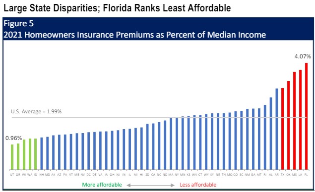
The IRC concluded that from 2001 to 2021, homeowners insurance expenditures showed a general upward trend, driven by factors such as natural disasters, economic conditions, rising construction costs, and litigation activity in some states. Meanwhile, the average household income also grew during the same time. However, the IRC found, the increase in insurance spend outpaces the increase in household income, with an annualized growth rate of 2.5%. It is important to note the report does not include the rapid increases in insurance rates since 2021, IRC said.

“An understanding of what drives the cost of insurance is essential for consumers navigating the current insurance market,” said Dale Porfilio, president of the IRC and chief insurance office for the Insurance Information Institute (Triple-I). “Efforts to promote homeowner awareness and adoption of protective measures, strengthen state and local building codes, and encourage community resilience programs can all improve insurance affordability.”

Topics Profit Loss Homeowners

Was this article valuable?

Thank you! Please tell us what we can do to improve this article.

Thank you! % of people found this article valuable. Please tell us what you liked about it.

Here are more articles you may enjoy.

Written By Chad Hemenway

Chad is National News Editor at Insurance Journal. He has been covering the insurance industry since 2007, reporting on trends and coverage in most lines of insurance as well as natural catastrophes, modeling, regulation, legislation, and litigation. Chad can be reached at [email protected]

Latest Posts:

• Fitch Ratings: US Cyber Premium Growth Slows in 2023
• Hospital Operator Ascension ‘Making Progress’ to Restore Systems After Cyberattack
• Berkshire’s Jain on Cyber: ‘The Mindset Should Be You’re Not Making Money’

Interested in Homeowners ?

Get automatic alerts for this topic.

• Categories: National News Topics: homeowners insurance , Insurance Research Council , Personal Lines , Research and Trends
• Have a hot lead? Email us at [email protected]

Insurance Jobs

• Junior Accountant - Fort Lee, NJ
• Outside Auto Appraiser- Sacramento, CA - Rancho Cordova, CA
• Select Sales Executive - Charlotte, NC
• Claim Rep, Worker’s Compensation Return To Work - Alpharetta, GA
• Client Advocate Financial Institutions & Professional Services - Atlanta, GA

• 3 Things to Know About Condo Association Boards
• Why Millennials and Gen Z Just Aren’t Loving Insurance: How Organizations Can Win the Next Generations of Insurance Consumers
• A Look at the Liquor Liability Landscape
• How to Sell Yacht Insurance Amidst a Rising Tide
• Squeezed from All Sides: Restaurants Pressured by Labor, Food, Insurance Costs

• Staffing Shortages, Reduced Safety Training Fuel Risks for Company Drivers
• U.S. Studying If Other Bridges at Risk After Baltimore Collapse
• Over 946,000 Customers Still Without Power After Storms in Texas, Louisiana
• AI Voiceover Company Stole Voices of Actors, New York Lawsuit Claims
• Spotify Accused in Suit of Cheating Songwriters Out of Royalties

• May 23 Broke as a Joke in 2024: Commercial Property Edition
• May 30 The US Legal System and Legal Liability
• June 6 Transit Risk in 2024
• June 13 Leading Modern Teams: Inclusive Leadership in Action

• Research article
• Open access
• Published: 07 May 2024

Floods and cause-specific mortality in the UK: a nested case-control study

• Danijela Gasevic 1 ,
• Zhengyu Yang 1 ,
• Guowei Zhou 2 ,
• Yan Zhang 2 ,
• Jiangning Song 3 ,
• Hong Liu 2   na1 ,
• Shanshan Li 2   na1 &
• Yuming Guo   ORCID: orcid.org/0000-0002-1766-6592 2   na1  

BMC Medicine volume  22 , Article number:  188 ( 2024 ) Cite this article

511 Accesses

18 Altmetric

Metrics details

Floods are the most frequent weather-related disaster, causing significant health impacts worldwide. Limited studies have examined the long-term consequences of flooding exposure.

Flood data were retrieved from the Dartmouth Flood Observatory and linked with health data from 499,487 UK Biobank participants. To calculate the annual cumulative flooding exposure, we multiplied the duration and severity of each flood event and then summed these values for each year. We conducted a nested case-control analysis to evaluate the long-term effect of flooding exposure on all-cause and cause-specific mortality. Each case was matched with eight controls. Flooding exposure was modelled using a distributed lag non-linear model to capture its nonlinear and lagged effects.

The risk of all-cause mortality increased by 6.7% (odds ratio (OR): 1.067, 95% confidence interval (CI): 1.063–1.071) for every unit increase in flood index after confounders had been controlled for. The mortality risk from neurological and mental diseases was negligible in the current year, but strongest in the lag years 3 and 4. By contrast, the risk of mortality from suicide was the strongest in the current year (OR: 1.018, 95% CI: 1.008–1.028), and attenuated to lag year 5. Participants with higher levels of education and household income had a higher estimated risk of death from most causes whereas the risk of suicide-related mortality was higher among participants who were obese, had lower household income, engaged in less physical activity, were non-moderate alcohol consumers, and those living in more deprived areas.

Conclusions

Long-term exposure to floods is associated with an increased risk of mortality. The health consequences of flooding exposure would vary across different periods after the event, with different profiles of vulnerable populations identified for different causes of death. These findings contribute to a better understanding of the long-term impacts of flooding exposure.

Peer Review reports

Floods are the most frequent type of weather-related disaster, accounting for about 47% of all weather-related disasters from 1995 to 2015 [ 1 , 2 ]. Between 1995 and 2015, more than 2.3 billion people were affected by flood disasters, with over 157 thousand people dying directly as a result of floods [ 3 ]. In recent years, many intense urban flooding events have been recorded in the UK, resulting in loss of lives, damages to personal property and public health infrastructure, and disruption to vital services such as water, communications, energy, and public transport [ 4 , 5 , 6 , 7 , 8 , 9 ]. Approximately 1.9 million people across the UK are at risk of floods, and this number will double as early as the 2050s [ 10 ].

In addition to immediate fatalities due to drowning and acute trauma [ 11 ], floods can also cause short- (lasting days or weeks) or medium-health impacts (several weeks or months), including the spread of water- and vector-borne diseases, such as cholera, typhoid, or malaria; injuries during evacuations and disaster clean-up; and exposure to chemical hazards [ 1 , 12 ]. Non-communicable diseases (e.g. cardiovascular disease, neoplasms, chronic respiratory diseases, and diabetes) which need prolonged treatment and care can be exacerbated after floods due to a disruption in care, treatment, medication, supplies, equipment, and overcrowding in shelters [ 13 , 14 , 15 , 16 , 17 , 18 ]. Mental health issues may arise from stressors caused by floods (e.g. property damage, financial loss, loss of a loved one) and have long-lasting health effects on mortality and morbidity. These long-term health consequences may arise from several pathways, including impairment of the immune system, sleep disturbances, substance abuse, and inadequate self-care [ 19 , 20 , 21 , 22 ].

Despite the severe impacts of floods, there currently is limited epidemiological evidence on the long-term mortality impacts of exposure to floods. To address these gaps in knowledge, we utilized the UK Biobank project, a population-based study with a large sample size, to explore the long-term effects of flooding on mortality. We aimed to estimate the risk of all-cause and seven cause-specific mortality associated with floods and to explore the lag patterns in mortality risk. We also conducted subgroup analyses to identify populations who are potentially more vulnerable to flood-related death.

Study design and study population

We conducted a nested case-control study within a cohort of participants registered with the UK Biobank study. About 0.5 million residents aged between 37 and 73 years were enrolled in the UK Biobank from 2006 to 2010, from 21 assessment centres across England, Wales, and Scotland. The cohort was followed up until the date of death or the study end date (December 31, 2020). We excluded participants lacking longitude and latitude data of residence ( n = 11), participants with missing data on age, sex, and ethnicity ( n = 2775), and those who died in the year of recruitment ( n = 141). A total of 499,487 participants were included (Fig 1 ). All participants in the UK Biobank study provided informed consent. The utilization of the data presented in this paper has been approved by the UK Biobank access committee under UK Biobank application number 55257.

A flow diagram to show participants whose data were used to estimate the association between flooding exposure and mortality

Case-control selection

With the nested case-control design, we matched controls to cases with replacement at the time of the outcome event and assessed exposure retrospectively, from the date of death or end of follow-up. This ensures identical exposure lengths across participants. Using a risk-set sampling method, each case was matched with eight controls randomly selected from study participants who met the matching criteria for age (within 5 years), sex (male and female), and ethnicity (White, Black, Asian or Asian British, mixed, Chinese, and others). The index date for cases corresponded to the date of death; while for controls, it was the date of death of the matched case participant. For twelve case-control sets, eligible controls were less than eight but at least one (Fig 1 ).

Participants were eligible for inclusion as cases for the study if they died during the study period. We defined all-cause mortality and seven cause-specific mortality categories using the International Classification of Diseases, edition 10 (ICD-10), classification as follows: neoplasms, C00–D48; cardiovascular disease, I00–I99; respiratory diseases, J09–J98; digestive disease, K20–K93; neurodegenerative disease, F01–03, G122, G20, G21, G23, G30, G31; mental and behavioural disorders: F00–F90; and suicide: X60–X84, Y10–Y34, Y87.

Flooding exposure

We collected flood data during 2000–2020 from the Dartmouth Flood Observatory (DFO), which is a global catalogue of all flood events with detailed information on start date, end date, centroids, impacted geographic areas, and severities. All documented flood events were sourced from news, government, and instrumental sources and have been validated by satellite observations [ 23 , 24 ]. Participants whose home addresses fall within flood-affected areas were considered as having been exposed to a flood event. To assess the long-term effect of floods, we calculated a cumulative exposure during the study period for each participant. Building on previous research [ 25 , 26 ], we derived the annual cumulative exposure by multiplying the duration and severity of each flood event and summing these values for each year. Our preliminary analyses suggested a weak negative association between flood severity and duration (Pearson coefficient: − 0.03). The severity of each flood event documented in the DFO was classified based on a pre-defined scale, detailed in Additional file 1 : Table S1. For each participant, annual cumulative flooding exposure was calculated using equation ( 1 ):

where \(\mathrm{Flood}\;{\mathrm{index}}_{i,\text{year}=m}\) stands for the cumulative flooding exposure in year \(m\) for participants \(i\) . \({{\text{Duration}}}_{ij}\) and \({{\text{Severity}}}_{ij}\) represent the duration (day) and the severity of the \(j\) th flood event that participant \(i\) experienced in year \(m\) , respectively. If there were no flood events within a given year, a flood index of 0 was recorded.

Meteorological data

We extracted hourly temperature and relative humidity data from the European Centre for Medium-Range Weather Forecasts Reanalysis v5 (ERA-5) reanalysis data set with a spatial resolution of 0.1°×0.1°. We mapped meteorological data to the participant’s geocoded residential address at baseline. Daily meteorological data were calculated by averaging hourly data within each day. Daily temperature and relative humidity were then aggregated into yearly averages.

Baseline data collected by the UK Biobank include demographics, lifestyle factors, socioeconomic status, and anthropometric measurements. We included additional covariates informed by existing literature, beyond those used for matching cases and controls [ 27 , 28 , 29 ]: body mass index (BMI), physical activity, healthy diet score, cigarette smoking, alcohol consumption, educational attainment, average total annual household income before tax, Townsend deprivation index (TDI), overall health rating, and assessment centres. BMI was calculated from objectively measured weight and height as weight over height squared and expressed as kg/m 2 . Physical activity was derived from the International Physical Activity Questionnaire-Short Form (IPAQ-SF) [ 30 ]. Participants were categorized at ‘high’ (≥ 1500 metabolic equivalent (MET)-minutes/week), ‘moderate’ (≥ 600 MET-minutes/week), or ‘low’ levels of physical activity following standardized IPAQ-SF scoring guidance [ 30 ]. Diet score was calculated based on the following dietary factors: vegetable intake ≥ 3 servings/day; fruit intake ≥ 3 servings /day; whole grains ≥ 3 servings/day; refined grains ≤ 1.5 servings/day; fish intake ≥ 2 servings/day; unprocessed red meat intake ≤ 2 servings/week; and processed meat intake ≤ 2 servings/week. Each point was given for each favourable dietary factor, and the suboptimal diet was defined as a diet score < 4. Smoking status was coded into three categories: current, former, and never. Low-risk alcohol consumption was defined as moderate drinking (no more than one drink/day for women and two drinks/day for men; one drink is measured as 8 g ethanol in the UK) on a relatively regular frequency [ 31 ]. Educational attainment was coded in two categories: ‘high’ (college or university degree) or ‘low’ (A/AS levels or equivalent, O levels/GCSEs or equivalent, or none of the above). Annual household income was classified into two groups (< £31,000 and ≥ £31,000). TDI was utilized to define area deprivation level, with participants being classified as either high (TDI above the median) or low [ 32 ]. Self-reported health was categorized as poor, fair, good, and excellent [ 27 ].

Statistical analysis

We performed conditional logistic regression analysis to estimate the risk of mortality associated with per unit increase in flood index. Year-specific flood index was modelled using a distributed lag non-linear model featuring a non-linear exposure-response association and the additional lag-response association, respectively [ 33 , 34 , 35 , 36 ]. The lag-response association refers to how the risk changes over time and provides an estimation of the combined immediate and delayed effects that accumulate throughout the lag period. We first modelled the exposure-response curve with a natural cubic spline with three degrees of freedom. However, the nonlinear analysis indicated an approximately linear relationship (Additional file 1 : Fig. S1). Further, both the Akaike Information Criterion (AIC) and the Bayesian Information Criterion (BIC) favoured the linear model (Additional file 1 : Table S2). Therefore, we applied a linear exposure-response relationship in the formal analysis. The lag-response curve was modelled with a natural cubic spline with three degrees of freedom plus an intercept. The exposure window comprised the 0 to 5 years before the index date. A maximum lag of 5 years was used because the flood-related mortality risk declined to zero by the lag year 5.

Estimates of risk were obtained from the crude model that only included flood (model 1); the multivariate model that additionally controlled for socioeconomic status (education attainment, household income, and deprivation) (model 2); and the full model that additionally adjusted for BMI, physical activity, smoking, alcohol consumption, suboptimal diet, overall health rating, mean temperature, mean relative humidity, and assessment centre which serves as an indicator of the recruitment location for each participant (model 3). All variance inflator factors were less than 1.5, indicating no multicollinearity. Temperature and relative humidity terms were defined as the average annual mean temperature and relative humidity over 6 years (lag 0–5 years) preceding the index date, respectively. Given that the crude model (model 1) did not include any covariates, all participants were retained in the analysis. For models 2 and 3, we excluded participants with any missing data. In sensitivity analyses, we employed multiple imputation to address missing covariate data and assess the robustness of our findings.

We further identified subgroups vulnerable to floods through stratification analyses by age group (≤64 and >65 years), sex, weight status defined according to BMI (≤ 24.9, 25–29.9, ≥ 30), education attainment, household income, physical activity, suboptimal diet, alcohol consumption status, smoking status, and area deprivation level. Results are presented as odds ratios (ORs) and their 95% confidence intervals (95% CIs) per unit increase in flood index. The significance of the difference in results between subgroups was tested using a random-effect meta-regression model.

Sensitivity analysis

We carried out the following sensitivity analyses: (1) Multiple imputation by chained equations was used for the missing values. Five imputed data sets were created, and their results were combined using Rubin’s rules [ 37 ]. (2) Alternative degrees of freedom were used for the lag-response association of flood. (3) Alternative degrees of freedom were used for the non-linear exposure-response relationship of mean temperature and relative humidity. (4) Alternative matching ratios (1:4 and 1:6) were used. (5) Excluding data after 2020 to control for the effect of the COVID-19 pandemic. (6) To capture the variation in flooding impacts within the year preceding mortality, we performed additional analyses with monthly flood index.

Table 1 shows the baseline characteristics of the 33,021 death cases and the 258,393 matched controls. The mean age (± standard deviation (SD)) of participants at study entry was 61.3 (± 6.4) years; 170,549 (58.5%) were male; 281,175 (96.5%) were white. Participants who died were more likely to have a higher BMI and lower household income; were less likely to be university graduates; more likely to smoke; and consumed less fruit and vegetables and more red and processed meat. They were also more likely to rate their overall health as poor and fair. Baseline characteristics of cases and controls with any missing values in covariates are shown in Additional file 1 : Table S3.

The distributions of the flood index and meteorological factors are shown in Table 2 . The annual average flood index across all participants during the study period ranged from 0.0 to 38.3, with a median value of 1.8 (25 th to 75 th percentiles: 0.5 to 3.6). Cases exposed to higher levels of flooding than controls during the 6 years before the end of follow-up (Additional file 1 : Fig. S2). The median annual mean temperature was 10.0 °C (25 th to 75 th percentiles: 9.3°C to 10.7°C) (Table 2 ). The flood index was negatively correlated with mean temperature (Pearson r = − 0.04) but positively correlated with relative humidity (Pearson r = 0.08).

Figure 2 illustrates the estimated cumulative OR of all-cause and cause-specific mortality associated with per unit increase in flood index over lag years 0–5. Per unit increase in flood index was associated with a 9.2% increased risk of all-cause mortality (OR: 1.092, 95% CI: 1.090–1.093) in the crude model. The results remained similar after further adjustment for socio-economic status (OR: 1.090, 95% CI: 1.088–1.091), whereas adjustment for lifestyle factors decreased the strength of the association (OR for fully adjusted model: 1.067, 95% CI: 1.063–1.071). Similar effects were observed for cause-specific mortality after fully adjusting the models, whereby a greater flood index was associated with a greater risk of death from neurodegenerative diseases (OR: 1.068, 95% CI: 1.050–1.087), neoplasm (OR: 1.063, 95% CI: 1.058–1.068), respiratory diseases (OR: 1.062, 95% CI: 1.045–1.080), suicide (OR: 1.052, 95% CI: 1.018–1.088), cardiovascular diseases (OR: 1.051, 95% CI: 1.042–1.059), mental diseases (OR: 1.047, 95% CI: 1.008–1.087), and digestive diseases (OR: 1.031, 95% CI: 1.011–1.052) (Fig. 2, Additional file 1 : Table S4).

Cumulative odds ratio of all-cause and cause-specific mortality associated with per unit increase in flood index over lag years 0–5. Estimates of risk were obtained from the crude model that only included flood (crude); the multivariate model that additionally controlled for socioeconomic status (education attainment, household income, and deprivation); and the full model that additionally adjusted for BMI, physical activity, smoking, alcohol consumption, suboptimal diet, overall health rating, mean temperature, mean relative humidity, and assessment centre which serves as an indicator of the recruitment location for each participant (fully adjusted). The error bars represent 95% confidence intervals

Figure 3 shows the lag structure in the effects of flooding exposure on all-cause and cause-specific mortality. For all-cause mortality, the magnitude of associations increased from the current year (OR: 1.012, 95% CI: 1.011–1.013) to the lag year 3 (OR: 1.016, 95% CI: 1.015–1.017), and subsequently diminished to zero by lag year 5. For neurodegenerative mortality and mortality due to mental-ill health, the mortality risk was negligible in the current year, but strongest in the lag years 3 and 4. By contrast, the risk of mortality from suicide was the strongest in the current year (OR: 1.018, 95% CI: 1.008–1.028), and attenuated to lag year 5.

Overall lag structure in effects of flooding exposure on cause-specific mortality. Shaded areas represent 95% confidence intervals for the odds ratio

Subgroup analyses revealed that participants with higher levels of education and household income had a higher estimated risk of death from most causes in association with flooding exposure. Participants aged below 64 and female had a higher estimated risk of death from all-cause mortality, respiratory diseases, and neoplasm, but a lower estimated risk of death from digestive and mental diseases, respectively. The risk of suicide-related mortality in association with flooding exposure was higher among participants who were obese, had lower household income, engaged in less physical activity, were non-moderate alcohol consumers, and had high deprivation levels (Table 3 ).

Our sensitivity analysis suggested that using multiple imputed data did not change study findings (Additional file 1 : Fig. S3). Our results were not dependent on modelling assumptions and remained unaffected by the COVID-19 pandemic (Additional file 1 : Fig. S4–7). Matching ratios of 1:4 and 1:6 revealed a modest increase in the odds ratio for all-cause mortality and neoplasms, while the odds ratio for other causes of death remained unchanged ( Additional file 1 : Fig. S8 ). For all-cause mortality, with per unit increase in monthly flood index, odds ratios over 0–12 months preceding the mortality ranged from 1.005 (95% CI: 1.005–1.006) to 1.018 (95% CI: 1.017–1.018) (Additional file 1 : Table S5).

In this nested case-control study, we observed a significantly increasing risk of mortality associated with floods. The exposure-response curve was linear, with no discernible thresholds. The lag pattern varied across different causes of death. Flooding exposure has a long-lasting impact on neurodegenerative and mental diseases, whereas it has an immediate impact on suicide. Subgroup analyses revealed specific groups of vulnerable populations for flood-related death, which varied according to the cause of death.

Every unit increase in flood index was associated with a 6.7% increase in all-cause mortality risk over the following 6 years. This finding was similar to cause-specific mortality. Although few epidemiological studies have assessed the long-term effect of floods on mortality, our findings are consistent with previous findings of short-term flooding exposure showing increased risk of cholera at lag 0–20 weeks [ 38 ], diarrhoea at lag 0–28 weeks [ 38 ], respiratory infection at lag 3 months [ 39 ], typhoid fever at lag 1 week [ 40 ], malaria at lag 1 year [ 12 ], malnutrition at lag 1 year [ 41 ], and mental disorders at lag 6 months [ 19 ]. One study assessing the effects of flooding on mortality in England and Wales during 1994–2005 suggested a deficit of deaths in the post-flood period [ 42 ]. The inconsistency might result from the underestimation of death number, which can occur when deaths are registered at different places after displacement and a short observation period (one year after flooding exposure) during which the occurrence of death has not been observed. Milojevic et al. reported a slight but non-significant increase in mortality rates following the floods in Bangladesh in the flooded areas compared to non-flooded areas [ 43 ]. The accuracy of their results might be subject to recall bias in exposure assessment, given that exposure to flooding was ascertained from an interview survey four years after the flood event.

The long-term health deterioration resulting from floods could be attributed to mental health disorders driven by financial losses and community or social disruption, especially for those who live in resource-poor countries and communities (e.g. floodplains or non-resistant buildings, lack of warning systems and awareness of flooding hazard) [ 1 , 44 ]. For example, previous studies reported a significant and continued increase in the prevalence of post-traumatic stress disorder (PTSD), stress, anxiety, depression, and even suicide ideation following flooding exposure [ 20 ], which contribute to worse health outcomes. Additionally, among people who were exposed to floods, those who had chronic medical conditions are at higher risk of health deterioration due to potential disruptions in medication and healthcare services. Previous studies have noted that older adults and those receiving long-term care services showed decreased treatment adherence (e.g. interruption of medication and access to physicians) months and even years after the flooding [ 45 , 46 ], which serve to exacerbate or prolong symptoms of existing conditions.

Flooding exposure has a long-lasting impact on neurodegenerative and mental diseases, reaching its peak at 3–4 years post-exposure whereas the highest risk of mortality due to suicide occurs in the year of exposure. This suggests that varying health issues should be given consideration, depending on the stage following flooding exposure. A study in Queensland has noted that direct exposure to flood resulted in an increase in alcohol and tobacco usage half a year after flooding [ 46 ] and use of substances has been associated with an increased risk of suicide attempts in previous studies [ 47 , 48 , 49 , 50 ]. However, social support and compensation coverage have been demonstrated to have had a positive impact on health [ 20 ], which helps reduce the risk of subsequent suicide attempts. By contrast, cognitive decline is more likely to occur 2 years later after natural disasters [ 51 , 52 ], resulting from the new onset of depression and disruption of social contacts (e.g. loss of interactions with neighbours) [ 51 ].

Our findings align with previous studies highlighting the vulnerability of cancer patients to disruptions in healthcare services following natural disasters. While limited evidence suggests an increased risk of disease exacerbation among cancer patients post-disaster, our primary concern is the potential for delays in receiving essential cancer care [ 14 , 18 ]. Natural disasters like floods can severely disrupt healthcare systems, leading to damage to oncology centres, loss of medical records, pharmaceutical shortages, displacement of healthcare workers, and disruptions in pathology specimen handling, all of which can compromise cancer patient care [ 13 , 53 , 54 , 55 , 56 ]. The relocation of cancer patients to temporary shelters can be particularly challenging and distressing, especially for those with clinical instability [ 53 ]. Additionally, initial recovery efforts following natural disasters often prioritize immediate needs such as providing shelter, food, water, and addressing injuries from environmental hazards, infectious diseases, or other acute conditions [ 57 ]. This prioritization of immediate needs may inadvertently overlook the continuity of care required for non-acute medical issues like cancer. Given the individualized and continuous nature of cancer treatment, neoplasms are particularly susceptible to the disruptions caused by natural disasters. Our study demonstrates the association between floods and elevated mortality risks among cancer patients, reinforcing the urgent need to prioritize the needs of cancer patients before, during, and after disasters [ 13 , 58 ].

Profiles of vulnerable populations to flood-related mortality varied across causes of death. Of all factors considered, socio-economic status, which is determined by individual levels of education and income, has been identified as a significant modifier of flood-related mortality impacts. Individuals with higher socioeconomic status tend to have an increased risk of flood-related mortality from chronic diseases (e.g. cardiovascular diseases, respiratory diseases, and neurodegenerative diseases) but decreased risk of flood-related mortality from suicide. Although there is very limited evidence that can elucidate this finding, some insights can be gathered from the following studies. It is reported that people in high socioeconomic groups are more likely to be affected by work-life conflict-induced mental illness due to their higher occupational aspirations but a greater discrepancy between aspirations and reality [ 59 , 60 ]. Flooding exposure may further amplify the disparity between an individual’s aspirations and their actual circumstances, resulting in a negative impact on their mental health. Long-lasting psychological illness has been associated with worse chronic medical conditions [ 61 ].

In our study, we observed that participants with higher BMI and lower physical activity levels exhibited a significantly higher risk of flood-related mortality from suicide, but a comparatively lower risk of all-cause mortality. These associations can be attributed to different factors. On the one hand, individuals in low socio-economic groups, those engaged in minimal physical activity, and non-moderate alcohol drinkers, are at higher risk of developing suicide ideation in a short time following psychological trauma associated with flooding exposure [ 49 , 62 ]. On the other hand, individuals with higher levels of physical activity may be prone to engage in risk-taking behaviours during flooding events, potentially leading to increased mortality rates [ 63 ]. These behaviours could involve actions such as entering floodwaters to cross a river or stream, safeguarding property and families (e.g. through activities like sandbagging homes and clearing drains), and participating in rescuing operations [ 63 ]. Surprisingly, current smokers demonstrated a decreased risk of flood-related mortality from all-cause deaths and neoplasms. We acknowledge that residual confounding, raising from unmeasured factors at follow-up, might contribute to these associations. Nevertheless, it is important to note that our study represents the first report of a higher mortality risk after long-term exposure to floods, highlighting the need for further investigations to validate this finding and explore potential underlying reasons.

Based on our research, flooding exposure is responsible for advancing a substantial number of deaths, with the impact persisting for up to 6 years. Our findings suggest that preventive interventions should be implemented peri- and post-flooding periods to reduce avoidable deaths due to flooding exposure. Following a flooding event, there is an increased risk of suicide within the first year. Therefore, timely provision of coping support and stress management is crucial to avert psychological illness, particularly among individuals in low socio-economic groups, those engaged in less physical activity, and non-moderate alcohol drinkers. In long-term rehabilitation, more resources should be allocated towards addressing the chronic medical conditions of populations that have been exposed to flooding, especially neurological well-being. It is also crucial to pay attention to the high-income population, although further research is needed to elucidate the underlying mechanisms behind their greater mortality risks associated with flooding exposure.

The limitations merit consideration. Our participants were residents in the UK who were more likely to live in less socioeconomically deprived areas, therefore, our results may not be generalizable to a whole population, especially people in low- and middle-income countries. Like most of cohort studies, covariates were collected at enrolment in the biobank. Due to the limited information on behavioural changes after the baseline examinations, we are unable to exclude the effect of behavioural changes on the risk estimates. However, most of the covariates (e.g. socio-economic status) were considered as effect modifiers rather than confounders, therefore, any changes in these factors should not have a substantial impact on our estimates. While the flood index accounts for cumulative exposure, it does not yet capture the potential differential impacts of distinct flood phases (warning, event, post-event) on mortality. Further research with a short-term design would be helpful to investigate the impacts of distinct flood phases. The destructive power of floods can differ based on factors like terrain, altitude, water management, drainage, urbanization, and building design. Therefore, a single severity label for an entire flood event may not fully capture the nuances of varying local experiences. Further research is needed to refine our exposure assessment as more detailed data becomes available. Lastly, it is likely for people to move after flooding exposure, with or without moving back into their homes. We assumed that participants did not move, which may have underestimated the effect of floods if an individual moved from an area with a high risk of flooding to an area with a lower risk of flooding. However, exposure to flooding can still have a long-term impact on them due to potential property damage and financial loss, even if people relocate to areas with a low risk of flooding in the aftermath of the event.

In conclusion, this study provides robust epidemiological evidence for associations of long-term exposure to flooding with increased risk of mortality. The health consequences of flooding exposure can vary across different periods after the event. These findings contribute to a better understanding of the long-term impacts of flooding exposure and can help improve public health practices to reduce the disease burden associated with floods.

Availability of data and materials

Data used in this study are available through registration on the UK Biobank.

Abbreviations

Akaike Information Criterion

Bayesian Information Criterion

Body mass index

Confidence interval    

Coronavirus disease 2019

Dartmouth Flood Observatory

European Centre for Medium-Range Weather Forecasts Reanalysis v5

International Classification of Diseases, edition 10

International Physical Activity Questionnaire-Short Form

Metabolic equivalent minutes per week

Post-traumatic stress disorder

Standard deviation

Townsend deprivation index

Lee J, Perera D, Glickman T, Taing LN. Water-related disasters and their health impacts: a global review. Prog Disaster Sci. 2020;8:100123.

Article   Google Scholar  

Wahlstrom M, Guha-Sapir D. The human cost of weather-related disasters 1995–2015. Geneva: UNISDR. 2015.

Wahlstrom M, Guha-Sapir D. The human cost of natural disasters: a global perspective. Geneva: UNISDR. 2015.

Rubinato M, Nichols A, Peng Y, Zhang JM, Lashford C, Cai YP, et al. Urban and river flooding: Comparison of flood risk management approaches in the UK and China and an assessment of future knowledge needs. Water Sci Eng. 2019;12(4):274–83.

Pitt M. Learning Lessons From the 2007 Floods. An Independent Review by Sir Michael Pitt. Cabinet Office, London. 2008.

Pregnolato M, Ford A, Wilkinson SM, Dawson RJ. The impact of flooding on road transport: A depth-disruption function. Transp Res D Transp Environ. 2017;55:67–81.

Thorne C. Geographies of UK flooding in 2013/4. Geogr J. 2014;180(4):297–309.

Marsh T, Kirby C, Muchan K, Barker L, Henderson E, Hannaford J. The winter floods of 2015/2016 in the UK-a review: UK:  NERC/Centre for Ecology and Hydrology; 2016.

Wallemacq P, Below R, McClean D. Economic losses, poverty and disasters: 1998-2017: Geneva: United Nations Office for Disaster Risk Reduction; 2018.

Sayers P, Horritt M, Carr S, Kay A, Mauz J, Lamb R, et al. Third UK Climate Change Risk Assessment (CCRA3): Future flood risk. UK: Research undertaken by Sayers and Partners for the Committee on Climate Change; 2020.

Jonkman SN, Kelman I. An analysis of the causes and circumstances of flood disaster deaths. Disasters. 2005;29(1):75–97.

Article   PubMed   Google Scholar  

Boyce R, Reyes R, Matte M, Ntaro M, Mulogo E, Metlay JP, et al. Severe Flooding and Malaria Transmission in the Western Ugandan Highlands: Implications for Disease Control in an Era of Global Climate Change. J Infect Dis. 2016;214(9):1403–10.

Article   PubMed   PubMed Central   Google Scholar  

Man RX, Lack DA, Wyatt CE, Murray V. The effect of natural disasters on cancer care: a systematic review. Lancet Oncol. 2018;19(9):e482–99.

Ryan B, Franklin RC, Burkle FM Jr, Aitken P, Smith E, Watt K, et al. Identifying and Describing the Impact of Cyclone, Storm and Flood Related Disasters on Treatment Management, Care and Exacerbations of Non-communicable Diseases and the Implications for Public Health. PLoS Curr. 2015;7:21–50.

Google Scholar  

McKinney N, Houser C, Meyer-Arendt K. Direct and indirect mortality in Florida during the 2004 hurricane season. Int J Biometeorol. 2011;55(4):533–46.

Rath B, Young EA, Harris A, Perrin K, Bronfin DR, Ratarh R, et al. Adverse Respiratory Symptoms and Environmental Exposures Among Children and Adolescents Following Hurricane Katrina. Public Health Rep. 2011;126(6):853–60.

Buajaroen H. Management of health care services for flood victims: The case of the shelter at Nakhon Pathom Rajabhat University Central Thailand. Australas Emerg Nurs. 2013;16(3):116–22.

Loehn B, Pou AM, Nuss DW, Tenney J, McWhorter A, DiLeo M, et al. Factors affecting access to head and neck cancer care after a natural disaster: a post-Hurricane Katrina survey. Head Neck. 2011;33(1):37–44.

Alderman K, Turner LR, Tong S. Assessment of the health impacts of the 2011 summer floods in Brisbane. Disaster Med Public Health Prep. 2013;7(4):380–6.

Zhong S, Yang L, Toloo S, Wang Z, Tong S, Sun X, et al. The long-term physical and psychological health impacts of flooding: A systematic mapping. Sci Total Environ. 2018;626:165–94.

Article   CAS   PubMed   Google Scholar  

Trief PM, Ouimette P, Wade M, Shanahan P, Weinstock RS. Post-traumatic stress disorder and diabetes: co-morbidity and outcomes in a male veterans sample. J Behav Med. 2006;29(5):411–8.

Sharpe I, Davison CM. Climate change, climate-related disasters and mental disorder in low- and middle-income countries: a scoping review. BMJ Open. 2021;11(10):e051908.

Carozza DA, Boudreault M. A global flood risk modeling framework built with climate models and machine learning. J Adv Model Earth Syst. 2021;13(4):e2020MS002221.

Yang Z, Huang W, McKenzie JE, Xu R, Yu P, Ye T, et al. Mortality risks associated with floods in 761 communities worldwide: time series study. BMJ. 2023;383:e075081.

Steenland K, Seals R, Klein M, Jinot J, Kahn HD. Risk estimation with epidemiologic data when response attenuates at high-exposure levels. Environ Health Perspect. 2011;119(6):831–7.

White E, Hunt JR, Casso D. Exposure measurement in cohort studies: the challenges of prospective data collection. Epidemiol Rev. 1998;20(1):43–56.

Ganna A, Ingelsson E. 5 year mortality predictors in 498,103 UK Biobank participants: a prospective population-based study. Lancet. 2015;386(9993):533–40.

Wang M, Zhou T, Song Q, Ma H, Hu Y, Heianza Y, et al. Ambient air pollution, healthy diet and vegetable intakes, and mortality: a prospective UK Biobank study. Int J Epidemiol. 2022;51(4):1243–53.

Wang M, Zhou T, Song Y, Li X, Ma H, Hu Y, et al. Joint exposure to various ambient air pollutants and incident heart failure: a prospective analysis in UK Biobank. European heart journal. 2021;42(16):1582–91.

Article   CAS   PubMed   PubMed Central   Google Scholar  

IPAQ Research Committee. Guidelines for data processing and analysis of the International Physical Activity Questionnaire (IPAQ)-short and long forms. https://www.physio-pedia.com/images/c/c7/Quidelines_for_interpreting_the_IPAQ.pdf (accessed January 20, 2024).

Zhang YB, Chen C, Pan XF, Guo J, Li Y, Franco OH, et al. Associations of healthy lifestyle and socioeconomic status with mortality and incident cardiovascular disease: two prospective cohort studies. BMJ. 2021;373:n604.

Chen H, Cao Y, Ma Y, Xu W, Zong G, Yuan C. Age- and sex-specific modifiable risk factor profiles of dementia: evidence from the UK Biobank. Eur J Epidemiol. 2023;38(1):83–93.

Jung CR, Chung WT, Chen WT, Lee RY, Hwang BF. Long-term exposure to traffic-related air pollution and systemic lupus erythematosus in Taiwan: A cohort study. Sci Total Environ. 2019;668:342–9.

Gasparrini A. Modeling exposure-lag-response associations with distributed lag non-linear models. Stat Med. 2014;33(5):881–99.

Li Y-Z, Huang S-H, Shi S, Chen W-X, Wei Y-F, Zou B-J, et al. Association of long-term particulate matter exposure with all-cause mortality among patients with ovarian cancer: A prospective cohort. Sci Total Environ. 2023;884:163748.

Kriit HK, Andersson EM, Carlsen HK, Andersson N, Ljungman PL, Pershagen G, et al. Using distributed lag non-linear models to estimate exposure lag-response associations between long-term air pollution exposure and incidence of cardiovascular disease. Int J Env Res Pub He. 2022;19(5):2630.

Article   CAS   Google Scholar  

Rubin DB. Multiple imputation for nonresponse in surveys: Canada: Wiley; 2004.

Hashizume M, Wagatsuma Y, Faruque ASG, Hayashi T, Hunter PR, Armstrong B, et al. Factors determining vulnerability to diarrhoea during and after severe floods in Bangladesh. J Water Health. 2008;6(3):323–32.

Saulnier DD, Hanson C, Ir P, Alvesson HM, von Schreeb J. The Effect of Seasonal Floods on Health: Analysis of Six Years of National Health Data and Flood Maps. Int J Env Res Pub He. 2018;15(4):665–77.

Liu ZD, Lao JH, Zhang Y, Liu YY, Zhang J, Wang H, et al. Association between floods and typhoid fever in Yongzhou, China: Effects and vulnerable groups. Environ Res. 2018;167:718–24.

Rodriguez-Llanes JM, Ranjan-Dash S, Mukhopadhyay A, Guha-Sapir D. Flood-Exposure Is Associated with Higher Prevalence of Child Undernutrition in Rural Eastern India. Int J Env Res Pub He. 2016;13(2):210.

Milojevic A, Armstrong B, Kovats S, Butler B, Hayes E, Leonardi G, et al. Long-term effects of flooding on mortality in England and Wales, 1994–2005: controlled interrupted time-series analysis. Environ Health. 2011;10(1):11–9.

Milojevic A, Armstrong B, Hashizume M, McAllister K, Faruque A, Yunus M, et al. Health Effects of Flooding in Rural Bangladesh. Epidemiology. 2012;23(1):107–15.

Ahern M, Kovats RS, Wilkinson P, Few R, Matthies F. Global health impacts of floods: Epidemiologic evidence. Epidemiol Rev. 2005;27:36–46.

Tomio J, Sato H, Mizumura H. Interruption of Medication among Outpatients with Chronic Conditions after a Flood. Prehospital Disaster. 2010;25(1):42–50.

Turner LR, Alderman K, Huang CR, Tong SL. Impact of the 2011 Queensland floods on the use of tobacco, alcohol and medication. Aust Nz J Publ Heal. 2013;37(4):396.

Orri M, Seguin JR, Castellanos-Ryan N, Tremblay RE, Cote SM, Turecki G, et al. A genetically informed study on the association of cannabis, alcohol, and tobacco smoking with suicide attempt. Mol Psychiatr. 2021;26(9):5061–70.

Berlin I, Hakes JK, Hu MC, Covey LS. Tobacco Use and Suicide Attempt: Longitudinal Analysis with Retrospective Reports. Plos One. 2015;10(4):e0122607.

Darvishi N, Farhadi M, Haghtalab T, Poorolajal J. Alcohol-Related Risk of Suicidal Ideation, Suicide Attempt, and Completed Suicide: A Meta-Analysis. Plos One. 2015;10(5):e0126870.

Gobbi G, Atkin T, Zytynski T. Association of Cannabis Use in Adolescence and Risk of Depression, Anxiety, and Suicidality in Young Adulthood: A Systematic Review and Meta-analysis. Jama Psychiat. 2019;76(4):426–34.

Hikichi H, Aida J, Kondo K, Tsuboya T, Matsuyama Y, Subramanian SV, et al. Increased risk of dementia in the aftermath of the 2011 Great East Japan Earthquake and Tsunami. P Natl Acad Sci USA. 2016;113(45):E6911–8.

Akanuma K, Nakamura K, Meguro K, Chiba M, Gutierrez Ubeda SR, Kumai K, et al. Disturbed social recognition and impaired risk judgement in older residents with mild cognitive impairment after the Great East Japan Earthquake of 2011: the Tome Project. Psychogeriatrics. 2016;16(6):349–54.

Morikawa N, Yanagisawa S, Iwasashi H, Tabata T, Abe T, Nakamura R, et al. Cancer patients in the hospital damaged by the Japan earthquake and tsunami. J Clin Oncol. 2012;30(15):e19508-e.

Cancer Ullman K, Disasters Care During Natural. J Natl Cancer I. 2011;103(24):1819–20.

Arrieta MI, Foreman RD, Crook ED, Icenogle ML. Providing Continuity of Care for Chronic Diseases in the Aftermath of Katrina: From Field Experience to Policy Recommendations. Disaster Med Public. 2009;3(3):174–82.

Rosenthal E. How the Cancer Community Fared During Hurricane Sandy's Mid-Atlantic Sweep. Oncology Times. 2012;34(23):8-10.

Prasad AS, Francescutti LH. Natural disasters. International encyclopedia of public health. 2017;5:215-22.

Aitsi-Selmi A, Murray V. Protecting the Health and Well-being of Populations from Disasters: Health and Health Care in The Sendai Framework for Disaster Risk Reduction 2015–2030. Prehospital Disaster. 2016;31(1):74–8.

Cochran DB, Wang EW, Stevenson SJ, Johnson LE, Crews C. Adolescent Occupational Aspirations: Test of Gottfredson’s Theory of Circumscription and Compromise. Career Dev Q. 2011;59(5):412–27.

Kim YM, Cho SI. Socioeconomic status, work-life conflict, and mental health. Am J Ind Med. 2020;63(8):703–12.

Patten SB, Williams JVA, Lavorato DH, Modgill G, Jette N, Eliasziw M. Major depression as a risk factor for chronic disease incidence: longitudinal analyses in a general population cohort. Gen Hosp Psychiat. 2008;30(5):407–13.

Vancampfort D, Hallgren M, Firth J, Rosenbaum S, Schuch FB, Mugisha J, et al. Physical activity and suicidal ideation: A systematic review and meta-analysis. J Affect Disorders. 2018;225:438–48.

Hamilton K, Demant D, Peden AE, Hagger MS. A systematic review of human behaviour in and around floodwater. Int J Disaster Risk Reduction. 2020;47:101561.

Download references

Acknowledgements

We gratefully thank all the participants in the UK Biobank, and everyone involved in planning and conducting the study.

Australian Research Council grant DP210102076

Australian National Health and Medical Research Council grant GNT2000581)

China Scholarship Council grant 202006010044 (YW)

China Scholarship Council grant 202006010043 (BW)

China Scholarship Council grant 201906210065 (PY)

National Health and Medical Research Council grant GNT2009866 (SL)

National Health and. Medical Research Council grant GNT1163693 (YG)

National Health and Medical Research Council grant GNT2008813 (YG)

Author information

Hong Liu, Shanshan Li, and Yuming Guo are co-senior authors.

Authors and Affiliations

School of Public Health and Preventive Medicine, Monash University, Level 2, 553 St Kilda Road, Melbourne, VIC, 3004, Australia

Yao Wu, Danijela Gasevic, Bo Wen, Zhengyu Yang & Pei Yu

Department of Dermatology, Xiangya Hospital, Central South University, Changsha, 410008, Hunan, China

Guowei Zhou, Yan Zhang, Hong Liu, Shanshan Li & Yuming Guo

Department of Biochemistry and Molecular Biology, Monash Biomedicine Discovery Institute, Monash University, Melbourne, VIC, 3800, Australia

Jiangning Song

You can also search for this author in PubMed   Google Scholar

Contributions

Conceptualization: YG, JS, HL, SL, YW. Methodology: YW, DG. Data collection: BW, ZY, GZ, YZ, ZY

Visualization: YW, BW. Supervision: YG, HL, SL. Writing—original draft: YW. Writing—review and editing: DG, BW, ZY, PY. All authors read and approved the final manuscript.

Authors’ Twitter handles

Yuming Guo: @YumingGuo007

Yao Wu: @Yaoyaowu13

Corresponding author

Correspondence to Yuming Guo .

Ethics declarations

Ethics approval and consent to participate.

UK Biobank has ethical approval from the North West Multi-Centre Research Ethics Committee (reference 16/NW/0274).

Consent for publication

Consent for publication was obtained from all included participants.

Competing interests

The authors declare that they have no competing interests.

Additional information

Publisher’s note.

Springer Nature remains neutral with regard to jurisdictional claims in published maps and institutional affiliations.

Supplementary Information

Additional file 1:.

Table S1. Definitions of different severities of flood events. Table S2. The Akaike Information Criterion (AIC) and the Bayesian Information Criterion (BIC) of nonlinear and linear models. Table S3. Baseline characteristics of cases and matched controls enrolled in UK Biobank, including missing values. Table S4. Cumulative odds ratios of cause-specific mortality associated with per unit increase in flood index over lag years 0–5. Table S5. Cumulative odds ratios of all-cause mortality associated with per unit increase in monthly flood index over lag month 0–12. Figure S1. Nonlinear curves of the associations between flood index and all-cause and cause-specific mortality. Figure S2. Cumulative flood index of cases and controls during the six years before the date of death or the end of the follow-up. Figure S3. Cumulative odds ratios of all-cause and cause-specific mortality associated with per unit increase in flood index over lag years 0–5 using complete data after multiple imputation. Figure S4. Cumulative odds ratios of all-cause and cause-specific mortality associated with per unit increase in flood index over lag years 0–5 using different degrees of freedom for lag-response association of flood index. Figure S5. Cumulative odds ratios of all-cause and cause-specific mortality associated with per unit increase in flood index over lag years 0–5 using different degrees of freedom for mean temperature. Figure S6. Cumulative odds ratios of all-cause and cause-specific mortality associated with per unit increase in flood index over lag years 0–5 using different degrees of freedom for relative humidity. Figure S7. Cumulative odds ratios of all-cause and cause-specific mortality associated with per unit increase in flood index over lag years 0–5 after excluding deaths after 2020. Figure S8. Cumulative odds ratios of all-cause and cause-specific mortality associated with per unit increase in flood index over lag years 0–5 using different matching ratios.

Rights and permissions

Open Access This article is licensed under a Creative Commons Attribution 4.0 International License, which permits use, sharing, adaptation, distribution and reproduction in any medium or format, as long as you give appropriate credit to the original author(s) and the source, provide a link to the Creative Commons licence, and indicate if changes were made. The images or other third party material in this article are included in the article's Creative Commons licence, unless indicated otherwise in a credit line to the material. If material is not included in the article's Creative Commons licence and your intended use is not permitted by statutory regulation or exceeds the permitted use, you will need to obtain permission directly from the copyright holder. To view a copy of this licence, visit http://creativecommons.org/licenses/by/4.0/ . The Creative Commons Public Domain Dedication waiver ( http://creativecommons.org/publicdomain/zero/1.0/ ) applies to the data made available in this article, unless otherwise stated in a credit line to the data.

Reprints and permissions

About this article

Cite this article.

Wu, Y., Gasevic, D., Wen, B. et al. Floods and cause-specific mortality in the UK: a nested case-control study. BMC Med 22 , 188 (2024). https://doi.org/10.1186/s12916-024-03412-0

Download citation

Received : 27 November 2023

Accepted : 29 April 2024

Published : 07 May 2024

DOI : https://doi.org/10.1186/s12916-024-03412-0

Share this article

Anyone you share the following link with will be able to read this content:

Sorry, a shareable link is not currently available for this article.

Provided by the Springer Nature SharedIt content-sharing initiative

• Natural disaster

BMC Medicine

ISSN: 1741-7015

• Submission enquiries: [email protected]
• General enquiries: [email protected]