convergence hypothesis is based on

This website uses cookies.

By clicking the "Accept" button or continuing to browse our site, you agree to first-party and session-only cookies being stored on your device to enhance site navigation and analyze site performance and traffic. For more information on our use of cookies, please see our Privacy Policy .

Research Highlights

The convergence hypothesis

April 6, 2020

Are poor countries catching up with rich countries?

Tyler Smith

The economies of today’s wealthiest nations raced ahead of the rest of the world about two centuries ago. That event initiated a new era in economic history, one defined by growth.

More recently, countries like Japan seem to have successfully copied this playbook, and it appears others like China are following suit. But unfortunately those countries are the exception rather than the rule, according to a paper in the Journal of Economic Literature .

Authors Paul Johnson and Chris Papageorgiou found there’s little evidence that national economies are catching up to their richest peers. Most low-income countries haven’t been able to maintain what growth spurts they’ve had like traditional economic theory would predict.

“The consensus that we find in the literature leads us to believe that poor countries, unless something changes, are destined to stay poor,” Johnson told the AEA in an interview.

In fact, slowdowns in the poorest countries have left millions in extreme poverty . Understanding which countries are catching up and how they’re doing so could help explain the elusive origins of economic growth.

The consensus that we find in the literature leads us to believe that poor countries, unless something changes, are destined to stay poor. Paul Johnson

The debate over catch-up growth—what economists have dubbed the convergence hypothesis —has a long history. The authors choose to focus on research published over the last 30 years.

In this recent research, capital, technology, and productivity have been at the root of most understandings of economic growth and convergence. But that has traditionally led economists to conclude that however poor a country starts off, it will adopt the best practices of the rich countries and eventually be just as well-off as their forerunners.

That’s the theory. But when the authors looked at the numbers over the last 60 years that’s not what they saw.

Data from the Penn World Tables —which covers 182 countries—revealed an unprecedented level of global growth over the period, but it was spread unevenly across the globe and across income levels.

The researchers separated countries into three income levels: low, middle, and high.

Each decade, high-income countries tended to grow faster than middle-income countries, which in turn tended to grow faster than low-income countries.

Every group experienced periods of relatively slow growth. But low-income countries actually experienced negative average growth rates during the 80s and 90s. The contractions were mostly driven by periods of extreme violence, corruption, and other state dysfunctions.

This unequal growth has led to steadily more and more dispersed national incomes around the world—the opposite of what a strong version of the convergence hypothesis predicts.

But while there wasn’t any absolute convergence, the researchers did find that the literature supported the idea of “convergence clubs.” In other words, countries that started with a similar income level in 1960 still had a similar income level in 2010, the end of the dataset.

The convergence clubs might be a clue for national leaders. According to Johnson, it suggests that policy interventions need to be bold enough to reach the next rung in the income ladder, or they risk slow, start-and-stop growth.

It also might help make sense of why some countries jump out of low-income clubs and eventually join the richest one, while other countries are stuck in poverty or middle-income traps.

Still other types of convergence are possible. Previous work has found that within some industries, such as manufacturing, convergence is happening. Countries may need to organize their workforces around these sectors to jumpstart growth.

As the authors point out, even half a century is short compared to the long run. The limited data span may mean that pessimism isn’t ultimately warranted, but the authors’ work warns against being complacent.

“There have been signs of a little catch-up over the last few years . . . but we don't know if that will continue,” Johnson said.

“ What Remains of Cross-Country Convergence? ” appears in the March issue of the Journal of Economic Literature.

The Great Divergence

This video explains how technology diffusion contributes to the growing productivity gap between rich and poor countries.

Can pathogen concentrations explain which countries developed sooner?

A new unified growth model of the demographic transition

Academia.edu no longer supports Internet Explorer.

To browse Academia.edu and the wider internet faster and more securely, please take a few seconds to upgrade your browser .

Enter the email address you signed up with and we'll email you a reset link.

We're Hiring!
Help Center

The convergence hypothesis: History, theory, and evidence

1998, Open economies review

Related Papers

Applied Economics Letters

Gerry Boyle

SSRN Electronic Journal

Shlomo Yitzhaki

Sandra Quijada

Economics Bulletin

This paper takes a closer look at the typical growth convergence regression of Barro (1991), Mankiw, Romer and Weil (1992), Sala-i-Martin (1996), and others. By interpreting the two components of the regression coefi¬ cient separately, i.e. the correlation coefficient and the ratio of standard deviations, we distinguish between "time-series" convergence and "cross-section" convergence, and consequently the relationship between I²âˆ’ and Iƒâˆ’convergence. And, using data from the latest Penn World Table database (version 9.1), we investigate the convergence or the lack-of-convergence in samples of countries representing the â€œWorldâ€ , OECD and Sub-Saharan Africa. The implications of this study for the neoclassical growth model are also discussed.

Angel De la Fuente

Jeffrey Sachs

KALSOOM ZULFIQAR

Convergence debate has been an important topic of economic growth literature. This article aims to investigate convergence at assorted level of disaggregation among a sample of almost 60 countries. It has tested absolute and conditional convergence hypotheses for a set of developed and developing countries by applying pooled least square methodology. The results suggest absolute convergence for countries having similar characteristics and conditional convergence for countries having heterogeneous structures. Disparity level for each country is also calculated with reference to average steady state income. The study has also scrutinized the role of investment, openness and population growth in accelerating the convergence process.

Annali d’Italia, scientific journal of Italy, №13, VOLUME 1, Florence, Italy

Karen Grigoryan

This paper analyzes the nature, causes, and consequences of income convergence in developing countries, and their attempt to catch-up with developed countries. It also addresses the question of sustainability of the convergence in the near future. In the context of income convergence, the relevance of productivity and welfare growth are discussed as indicators of convergence. The paper examines the catch-up growth and convergence approaches in the example of Armenia as a developing economy.

Robert Waldmann

Journal of Yaşar University

Burak Camurdan

In this paper, we study the GDP per capita convergence in emerging market economies for the period of 1950-2008. As the convergence in emerging market economies hasn’t been concerned as much as in the developed countries in the literature, hereby the situation of the convergence in emerging market economies is tried to be found out by the investigation. For this purpose, GDP per capita convergences in 25 developing countries were tested by ADF unit root test, Nahar and Inder (2002) Test and Kapetanios, Snell, and Shin (KSS) (2003) Test, which is based on the non-linear time series technique. While ADF unit root test allows to infer that there is convergence upon to the used series are stationary, the Nahar and Inder (2002) Test asserts that the existence of the convergence could also infer whether the used series are not stationary. On the other hand, the Kapetanios, Snell, and Shin (KSS) (2003) Test reveals that, if non-linear time series are stationary, the convergence could be in...

RELATED PAPERS

Maheep Bhatnagar

Tudásmenedzsment

Daniella Tirner

Indian Pediatrics

Narayanan Namboodiri

Journal of Research and Applications in Agricultural Engineering

Tomasz Sekutowski

Thuto Mosuang

Arquivos de Neuro-Psiquiatria

Raquel Gomes

Cecilia Ros

Ronald Evans

Önder Sezer

Proceedings of the Thirtieth International Joint Conference on Artificial Intelligence

Xiaocheng Feng

Filosofía y ciencia: reflexiones contemporáneas

Luisa Gonzalez-Reiche

Rev. nefrol. diálisis …

Nestor Lago

Journal of Pineal Research

Gerhard Heldmaier

Wilson Senne

Lenka Vrablikova

ChemistrySelect

Bekir Salih

Applied mathematical sciences

Ibrahim Massy

Infectious diseases

GIUSI MACALUSO

Ankara üniversitesi eğitim bilimleri fakültesi özel eğitim dergisi

Frontiers in Public Health

Aida Turrini

Arthroscopy Techniques

João Antonio Matheus Guimarães

Occupational Medicine

Susan Tarlo

ANA MARIA CALLES DOÑATE

Advances in Geometry

Mauro Nacinovich

David Kliger

1 Convergence Theory

Published: January 2002
Cite Icon Cite
Permissions Icon Permissions

This chapter discusses evidence for convergence theory, the idea that as rich countries got richer, they developed similar economic, political, and social structures and to some extent common values and beliefs. The analysis reveals that high levels of economic development and related changes in the occupational and industrial composition of the labor force result in two areas of convergence: the gradual spread of nonstandard schedules of work and the substantial and rapid growth of contingent labor in both manufacturing and service. Total annual hours of work declined from the late nineteenth century until about 1960, a trend that has continued in all rich democracies ever since.

Signed in as

Institutional accounts.

Google Scholar Indexing
GoogleCrawler [DO NOT DELETE]

Personal account

Sign in with email/username & password
Get email alerts
Save searches
Purchase content
Activate your purchase/trial code

Institutional access

Sign in with a library card Sign in with username/password Recommend to your librarian
Institutional account management
Get help with access

Access to content on Oxford Academic is often provided through institutional subscriptions and purchases. If you are a member of an institution with an active account, you may be able to access content in one of the following ways:

IP based access

Typically, access is provided across an institutional network to a range of IP addresses. This authentication occurs automatically, and it is not possible to sign out of an IP authenticated account.

Sign in through your institution

Choose this option to get remote access when outside your institution. Shibboleth/Open Athens technology is used to provide single sign-on between your institutionâ€™s website and Oxford Academic.

Click Sign in through your institution.
Select your institution from the list provided, which will take you to your institution's website to sign in.
When on the institution site, please use the credentials provided by your institution. Do not use an Oxford Academic personal account.
Following successful sign in, you will be returned to Oxford Academic.

If your institution is not listed or you cannot sign in to your institutionâ€™s website, please contact your librarian or administrator.

Sign in with a library card

Enter your library card number to sign in. If you cannot sign in, please contact your librarian.

Society Members

Society member access to a journal is achieved in one of the following ways:

Sign in through society site

Many societies offer single sign-on between the society website and Oxford Academic. If you see â€˜Sign in through society siteâ€™ in the sign in pane within a journal:

Click Sign in through society site.
When on the society site, please use the credentials provided by that society. Do not use an Oxford Academic personal account.

If you do not have a society account or have forgotten your username or password, please contact your society.

Sign in using a personal account

Some societies use Oxford Academic personal accounts to provide access to their members. See below.

A personal account can be used to get email alerts, save searches, purchase content, and activate subscriptions.

Some societies use Oxford Academic personal accounts to provide access to their members.

Viewing your signed in accounts

Click the account icon in the top right to:

View your signed in personal account and access account management features.
View the institutional accounts that are providing access.

Signed in but can't access content

Oxford Academic is home to a wide variety of products. The institutional subscription may not cover the content that you are trying to access. If you believe you should have access to that content, please contact your librarian.

For librarians and administrators, your personal account also provides access to institutional account management. Here you will find options to view and activate subscriptions, manage institutional settings and access options, access usage statistics, and more.

Our books are available by subscription or purchase to libraries and institutions.

About Oxford Academic
Publish journals with us
University press partners
What we publish
New features
Open access
Rights and permissions
Accessibility
Advertising
Media enquiries
Oxford University Press
Oxford Languages
University of Oxford

Oxford University Press is a department of the University of Oxford. It furthers the University's objective of excellence in research, scholarship, and education by publishing worldwide

Copyright © 2024 Oxford University Press
Cookie settings
Cookie policy
Privacy policy
Legal notice

This Feature Is Available To Subscribers Only

This PDF is available to Subscribers Only

For full access to this pdf, sign in to an existing account, or purchase an annual subscription.

20.4 Economic Convergence

Learning objectives.

By the end of this section, you will be able to:

Explain economic convergence
Analyze various arguments for and against economic convergence
Evaluate the speed of economic convergence between high-income countries and the rest of the world

Some low-income and middle-income economies around the world have shown a pattern of convergence , in which their economies grow faster than those of high-income countries. GDP increased by an average rate of 2.7% per year in the 1990s and 1.7% per year from 2010 to 2019 in the high-income countries of the world, which include the United States, Canada, the European Union countries, Japan, Australia, and New Zealand.

Table 20.5 lists eight countries that belong to an informal “fast growth club.” These countries averaged GDP growth (after adjusting for inflation) of at least 5% per year in both the time periods from 1990 to 2000 and from 2010 to 2019. Since economic growth in these countries has exceeded the average of the world’s high-income economies, these countries may converge with the high-income countries. The second part of Table 20.5 lists the “slow growth club,” which consists of countries that averaged GDP growth of 2% per year or less (after adjusting for inflation) during the same time periods. The final portion of Table 20.5 shows GDP growth rates for the countries of the world divided by income. (Note that the reason there is no data for 2001–2009 is because of the Great Recession, which lasted from 2007–2009. Many country’s GDP shrank during these years.)

Each of the countries in Table 20.5 has its own unique story of investments in human and physical capital, technological gains, market forces, government policies, and even lucky events, but an overall pattern of convergence is clear. The low-income countries have GDP growth that is faster than that of the middle-income countries, which in turn have GDP growth that is faster than that of the high-income countries. Two prominent members of the fast-growth club are China and India, which between them have nearly 40% of the world’s population. Some prominent members of the slow-growth club are high-income countries like France, Germany, Italy, and Japan.

Will this pattern of economic convergence persist into the future? This is a controversial question among economists that we will consider by looking at some of the main arguments on both sides.

Arguments Favoring Convergence

Several arguments suggest that low-income countries might have an advantage in achieving greater worker productivity and economic growth in the future.

A first argument is based on diminishing marginal returns. Even though deepening human and physical capital will tend to increase GDP per capita, the law of diminishing returns suggests that as an economy continues to increase its human and physical capital, the marginal gains to economic growth will diminish. For example, raising the average education level of the population by two years from a tenth-grade level to a high school diploma (while holding all other inputs constant) would produce a certain increase in output. An additional two-year increase, so that the average person had a two-year college degree, would increase output further, but the marginal gain would be smaller. Yet another additional two-year increase in the level of education, so that the average person would have a four-year-college bachelor’s degree, would increase output still further, but the marginal increase would again be smaller. A similar lesson holds for physical capital. If the quantity of physical capital available to the average worker increases, by, say, $5,000 to $10,000 (again, while holding all other inputs constant), it will increase the level of output. An additional increase from $10,000 to $15,000 will increase output further, but the marginal increase will be smaller.

Low-income countries like China and India tend to have lower levels of human capital and physical capital, so an investment in capital deepening should have a larger marginal effect in these countries than in high-income countries, where levels of human and physical capital are already relatively high. Diminishing returns implies that low-income economies could converge to the levels that the high-income countries achieve.

A second argument is that low-income countries may find it easier to improve their technologies than high-income countries. High-income countries must continually invent new technologies, whereas low-income countries can often find ways of applying technology that has already been invented and is well understood. The economist Alexander Gerschenkron (1904–1978) gave this phenomenon a memorable name: “the advantages of backwardness.” Of course, he did not literally mean that it is an advantage to have a lower standard of living. He was pointing out that a country that is behind has some extra potential for catching up.

Finally, optimists argue that many countries have observed the experience of those that have grown more quickly and have learned from it. Moreover, once the people of a country begin to enjoy the benefits of a higher standard of living, they may be more likely to build and support the market-friendly institutions that will help provide this standard of living.

View this video to learn about economic growth across the world.

Arguments That Convergence Is neither Inevitable nor Likely

If the economy's growth depended only on the deepening of human capital and physical capital, then we would expect that economy's growth rate to slow down over the long run because of diminishing marginal returns. However, there is another crucial factor in the aggregate production function: technology.

Developing new technology can provide a way for an economy to sidestep the diminishing marginal returns of capital deepening. Figure 20.7 shows how. The figure's horizontal axis measures the amount of capital deepening, which on this figure is an overall measure that includes deepening of both physical and human capital. The amount of human and physical capital per worker increases as you move from left to right, from C 1 to C 2 to C 3 . The diagram's vertical axis measures per capita output. Start by considering the lowest line in this diagram, labeled Technology 1. Along this aggregate production function, the level of technology is held constant, so the line shows only the relationship between capital deepening and output. As capital deepens from C 1 to C 2 to C 3 and the economy moves from R to U to W, per capita output does increase—but the way in which the line starts out steeper on the left but then flattens as it moves to the right shows the diminishing marginal returns, as additional marginal amounts of capital deepening increase output by ever-smaller amounts. The shape of the aggregate production line (Technology 1) shows that the ability of capital deepening, by itself, to generate sustained economic growth is limited, since diminishing returns will eventually set in.

Now, bring improvements in technology into the picture. Improved technology means that with a given set of inputs, more output is possible. The production function labeled Technology 1 in the figure is based on one level of technology, but Technology 2 is based on an improved level of technology, so for every level of capital deepening on the horizontal axis, it produces a higher level of output on the vertical axis. In turn, production function Technology 3 represents a still higher level of technology, so that for every level of inputs on the horizontal axis, it produces a higher level of output on the vertical axis than either of the other two aggregate production functions.

Most healthy, growing economies are deepening their human and physical capital and increasing technology at the same time. As a result, the economy can move from a choice like point R on the Technology 1 aggregate production line to a point like S on Technology 2 and a point like T on the still higher aggregate production line (Technology 3). With the combination of technology and capital deepening, the rise in GDP per capita in high-income countries does not need to fade away because of diminishing returns. The gains from technology can offset the diminishing returns involved with capital deepening.

Will technological improvements themselves run into diminishing returns over time? That is, will it become continually harder and more costly to discover new technological improvements? Perhaps someday, but, at least over the last two centuries since the beginning of the Industrial Revolution, improvements in technology have not run into diminishing marginal returns. Modern inventions, like the internet or discoveries in genetics or materials science, do not seem to provide smaller gains to output than earlier inventions like the steam engine or the railroad. One reason that technological ideas do not seem to run into diminishing returns is that we often can apply widely the ideas of new technology at a marginal cost that is very low or even zero. A specific worker or group of workers must use a specific additional machine, or an additional year of education. Many workers across the economy can use a new technology or invention at very low marginal cost.

The argument that it is easier for a low-income country to copy and adapt existing technology than it is for a high-income country to invent new technology is not necessarily true, either. When it comes to adapting and using new technology, a society’s performance is not necessarily guaranteed, but is the result of whether the country's economic, educational, and public policy institutions are supportive. In theory, perhaps, low-income countries have many opportunities to copy and adapt technology, but if they lack the appropriate supportive economic infrastructure and institutions, the theoretical possibility that backwardness might have certain advantages is of little practical relevance.

Visit this website to read more about economic growth in India.

The Slowness of Convergence

Although economic convergence between the high-income countries and the rest of the world seems possible and even likely, it will proceed slowly. Consider, for example, a country that starts off with a GDP per capita of $40,000, which would roughly represent a typical high-income country today, and another country that starts out at $4,000, which is roughly the level in low-income but not impoverished countries like Indonesia, Guatemala, or Egypt. Say that the rich country chugs along at a 2% annual growth rate of GDP per capita, while the poorer country grows at the aggressive rate of 7% per year. After 30 years, GDP per capita in the rich country will be $72,450 (that is, $40,000 (1 + 0.02) 30 ) while in the poor country it will be $30,450 (that is, $4,000 (1 + 0.07) 30 ). Convergence has occurred. The rich country used to be 10 times as wealthy as the poor one, and now it is only about 2.4 times as wealthy. Even after 30 consecutive years of very rapid growth, however, people in the low-income country are still likely to feel quite poor compared to people in the rich country. Moreover, as the poor country catches up, its opportunities for catch-up growth are reduced, and its growth rate may slow down somewhat.

The slowness of convergence illustrates again that small differences in annual rates of economic growth become huge differences over time. The high-income countries have been building up their advantage in standard of living over decades—more than a century in some cases. Even in an optimistic scenario, it will take decades for the low-income countries of the world to catch up significantly.

Bring It Home

Calories and economic growth.

We can tell the story of modern economic growth by looking at calorie consumption over time. The dramatic rise in incomes allowed the average person to eat better and consume more calories. How did these incomes increase? The neoclassical growth consensus uses the aggregate production function to suggest that the period of modern economic growth came about because of increases in inputs such as technology and physical and human capital. Also important was the way in which technological progress combined with physical and human capital deepening to create growth and convergence. The issue of distribution of income notwithstanding, it is clear that the average worker can afford more calories in 2020 than in 1875.

Aside from increases in income, there is another reason why the average person can afford more food. Modern agriculture has allowed many countries to produce more food than they need. Despite having more than enough food, however, many governments and multilateral agencies have not solved the food distribution problem. In fact, food shortages, famine, or general food insecurity are caused more often by the failure of government macroeconomic policy, according to the Nobel Prize-winning economist Amartya Sen. Sen has conducted extensive research into issues of inequality, poverty, and the role of government in improving standards of living. Macroeconomic policies that strive toward stable inflation, full employment, education of women, and preservation of property rights are more likely to eliminate starvation and provide for a more even distribution of food.

Because we have more food per capita, global food prices have decreased since 1875. The prices of some foods, however, have decreased more than the prices of others. For example, researchers from the University of Washington have shown that in the United States, calories from zucchini and lettuce are 100 times more expensive than calories from oil, butter, and sugar. Research from countries like India, China, and the United States suggests that as incomes rise, individuals want more calories from fats and protein and fewer from carbohydrates. This has very interesting implications for global food production, obesity, and environmental consequences. Affluent urban India has an obesity problem much like many parts of the United States. The forces of convergence are at work.

As an Amazon Associate we earn from qualifying purchases.

This book may not be used in the training of large language models or otherwise be ingested into large language models or generative AI offerings without OpenStax's permission.

Want to cite, share, or modify this book? This book uses the Creative Commons Attribution License and you must attribute OpenStax.

Access for free at https://openstax.org/books/principles-economics-3e/pages/1-introduction

Authors: Steven A. Greenlaw, David Shapiro, Daniel MacDonald
Publisher/website: OpenStax
Book title: Principles of Economics 3e
Publication date: Dec 14, 2022
Location: Houston, Texas
Book URL: https://openstax.org/books/principles-economics-3e/pages/1-introduction
Section URL: https://openstax.org/books/principles-economics-3e/pages/20-4-economic-convergence

© Jan 23, 2024 OpenStax. Textbook content produced by OpenStax is licensed under a Creative Commons Attribution License . The OpenStax name, OpenStax logo, OpenStax book covers, OpenStax CNX name, and OpenStax CNX logo are not subject to the Creative Commons license and may not be reproduced without the prior and express written consent of Rice University.

Subscriber Services
For Authors
Publications
Archaeology
Art & Architecture
Bilingual dictionaries
Classical studies
Encyclopedias
English Dictionaries and Thesauri
Language reference
Linguistics
Media studies
Medicine and health
Names studies
Performing arts
Science and technology
Social sciences
Society and culture
Overview Pages
Subject Reference
English Dictionaries
Bilingual Dictionaries

More Like This

Show all results sharing this subject:

convergence hypothesis

Quick reference.

The theory that socialism and capitalism will, over time, become increasingly alike in economic and social terms. Convergence theory was popular in the 1950s and 1960s, when Raymond Aron, John ...

From: convergence hypothesis in Dictionary of the Social Sciences »

Subjects: Social sciences

20.4 Economic Convergence

Learning objectives.

Explain economic convergence
Analyze various arguments for and against economic convergence
Evaluate the speed of economic convergence between high-income countries and the rest of the world

Some low-income and middle-income economies around the world have shown a pattern of convergence , in which their economies grow faster than those of high-income countries. GDP increased by an average rate of 2.7% per year in the 1990s and 2.3% per year from 2000 to 2008 in the high-income countries of the world, which include the United States, Canada, the countries of the European Union, Japan, Australia, and New Zealand.

Table 5 lists 10 countries of the world that belong to an informal “fast growth club.” These countries averaged GDP growth (after adjusting for inflation) of at least 5% per year in both the time periods from 1990 to 2000 and from 2000 to 2008. Since economic growth in these countries has exceeded the average of the world’s high-income economies, these countries may converge with the high-income countries. The second part of Table 5 lists the “slow growth club,” which consists of countries that averaged GDP growth of 2% per year or less (after adjusting for inflation) during the same time periods. The final portion of Table 5 shows GDP growth rates for the countries of the world divided by income.

Each of the countries in Table 5 has its own unique story of investments in human and physical capital, technological gains, market forces, government policies, and even lucky events, but an overall pattern of convergence is clear. The low-income countries have GDP growth that is faster than that of the middle-income countries, which in turn have GDP growth that is faster than that of the high-income countries. Two prominent members of the fast-growth club are China and India, which between them have nearly 40% of the world’s population. Some prominent members of the slow-growth club are high-income countries like the United States, France, Germany, Italy, and Japan.

Will this pattern of economic convergence persist into the future? This is a controversial question among economists that we will consider by looking at some of the main arguments on both sides.

Arguments Favoring Convergence

Several arguments suggest that low-income countries might have an advantage in achieving greater worker productivity and economic growth in the future.

View this video to learn about economic growth across the world.

Arguments That Convergence Is neither Inevitable nor Likely

If the growth of an economy depended only on the deepening of human capital and physical capital, then the growth rate of that economy would be expected to slow down over the long run because of diminishing marginal returns. However, there is another crucial factor in the aggregate production function: technology.

The development of new technology can provide a way for an economy to sidestep the diminishing marginal returns of capital deepening. Figure 1 shows how. The horizontal axis of the figure measures the amount of capital deepening, which on this figure is an overall measure that includes deepening of both physical and human capital. The amount of human and physical capital per worker increases as you move from left to right, from C 1 to C 2 to C 3 . The vertical axis of the diagram measures per capita output. Start by considering the lowest line in this diagram, labeled Technology 1. Along this aggregate production function, the level of technology is being held constant, so the line shows only the relationship between capital deepening and output. As capital deepens from C 1 to C 2 to C 3 and the economy moves from R to U to W, per capita output does increase—but the way in which the line starts out steeper on the left but then flattens as it moves to the right shows the diminishing marginal returns, as additional marginal amounts of capital deepening increase output by ever-smaller amounts. The shape of the aggregate production line (Technology 1) shows that the ability of capital deepening, by itself, to generate sustained economic growth is limited, since diminishing returns will eventually set in.

The graph shows three upward arching lines that each represent a different technology. Improvements in technology lead to greater output per capita and deepened physical and human capital.

Will technological improvements themselves run into diminishing returns over time? That is, will it become continually harder and more costly to discover new technological improvements? Perhaps someday, but, at least over the last two centuries since the Industrial Revolution, improvements in technology have not run into diminishing marginal returns. Modern inventions, like the Internet or discoveries in genetics or materials science, do not seem to provide smaller gains to output than earlier inventions like the steam engine or the railroad. One reason that technological ideas do not seem to run into diminishing returns is that the ideas of new technology can often be widely applied at a marginal cost that is very low or even zero. A specific additional machine, or an additional year of education, must be used by a specific worker or group of workers. A new technology or invention can be used by many workers across the economy at very low marginal cost.

The argument that it is easier for a low-income country to copy and adapt existing technology than it is for a high-income country to invent new technology is not necessarily true, either. When it comes to adapting and using new technology, a society’s performance is not necessarily guaranteed, but is the result of whether the economic, educational, and public policy institutions of the country are supportive. In theory, perhaps, low-income countries have many opportunities to copy and adapt technology, but if they lack the appropriate supportive economic infrastructure and institutions, the theoretical possibility that backwardness might have certain advantages is of little practical relevance.

Visit this website to read more about economic growth in India.

The Slowness of Convergence

Although economic convergence between the high-income countries and the rest of the world seems possible and even likely, it will proceed slowly. Consider, for example, a country that starts off with a GDP per capita of $40,000, which would roughly represent a typical high-income country today, and another country that starts out at $4,000, which is roughly the level in low-income but not impoverished countries like Indonesia, Guatemala, or Egypt. Say that the rich country chugs along at a 2% annual growth rate of GDP per capita, while the poorer country grows at the aggressive rate of 7% per year. After 30 years, GDP per capita in the rich country will be $72,450 (that is, $40,000 (1 + 0.02) 30 ) while in the poor country it will be $30,450 (that is, $4,000 (1 + 0.07) 30 ). Convergence has occurred; the rich country used to be 10 times as wealthy as the poor one, and now it is only about 2.4 times as wealthy. Even after 30 consecutive years of very rapid growth, however, people in the low-income country are still likely to feel quite poor compared to people in the rich country. Moreover, as the poor country catches up, its opportunities for catch-up growth are reduced, and its growth rate may slow down somewhat.

Calories and Economic Growth

The story of modern economic growth can be told by looking at calorie consumption over time. The dramatic rise in incomes allowed the average person to eat better and consume more calories. How did these incomes increase? The neoclassical growth consensus uses the aggregate production function to suggest that the period of modern economic growth came about because of increases in inputs such as technology and physical and human capital. Also important was the way in which technological progress combined with physical and human capital deepening to create growth and convergence. The issue of distribution of income notwithstanding, it is clear that the average worker can afford more calories in 2014 than in 1875.

Key Concepts and Summary

When countries with lower levels of GDP per capita catch up to countries with higher levels of GDP per capita, the process is called convergence. Convergence can occur even when both high- and low-income countries increase investment in physical and human capital with the objective of growing GDP. This is because the impact of new investment in physical and human capital on a low-income country may result in huge gains as new skills or equipment are combined with the labor force. In higher-income countries, however, a level of investment equal to that of the low income country is not likely to have as big an impact, because the more developed country most likely has high levels of capital investment. Therefore, the marginal gain from this additional investment tends to be successively less and less. Higher income countries are more likely to have diminishing returns to their investments and must continually invent new technologies; this allows lower-income economies to have a chance for convergent growth. However, many high-income economies have developed economic and political institutions that provide a healthy economic climate for an ongoing stream of technological innovations. Continuous technological innovation can counterbalance diminishing returns to investments in human and physical capital.

Self-Check Questions

Use an example to explain why, after periods of rapid growth, a low-income country that has not caught up to a high-income country may feel poor.
A weak economy in which businesses become reluctant to make long-term investments in physical capital.
A rise in international trade.
A trend in which many more adults participate in continuing education courses through their employers and at colleges and universities.
What are the “advantages of backwardness” for economic growth?
Would you expect capital deepening to result in diminished returns? Why or why not? Would you expect improvements in technology to result in diminished returns? Why or why not?
Why does productivity growth in high-income economies not slow down as it runs into diminishing returns from additional investments in physical capital and human capital? Does this show one area where the theory of diminishing returns fails to apply? Why or why not?

Review Questions

For a high-income economy like the United States, what elements of the aggregate production function are most important in bringing about growth in GDP per capita? What about a middle-income country such as Brazil? A low-income country such as Niger?
List some arguments for and against the likelihood of convergence.

Critical Thinking Questions

What sorts of policies can governments implement to encourage convergence?
As technological change makes us more sedentary and food costs increase, obesity is likely. What factors do you think may limit obesity?

Central Intelligence Agency. “The World Factbook: Country Comparison: GDP–Real Growth Rate.” https://www.cia.gov/library/publications/the-world-factbook/rankorder/2003rank.html.

Sen, Amartya. “Hunger in the Contemporary World (Discussion Paper DEDPS/8).” The Suntory Centre: London School of Economics and Political Science . Last modified November 1997. http://sticerd.lse.ac.uk/dps/de/dedps8.pdf.

Answers to Self-Check Questions

A good way to think about this is how a runner who has fallen behind in a race feels psychologically and physically as he catches up. Playing catch-up can be more taxing than maintaining one’s position at the head of the pack.
No. Capital deepening refers to an increase in the amount of capital per person in an economy. A decrease in investment by firms will actually cause the opposite of capital deepening (since the population will grow over time).
There is no direct connection between and increase in international trade and capital deepening. One could imagine particular scenarios where trade could lead to capital deepening (for example, if international capital inflows which are the counterpart to increasing the trade deficit) lead to an increase in physical capital investment), but in general, no.
Yes. Capital deepening refers to an increase in either physical capital or human capital per person. Continuing education or any time of lifelong learning adds to human capital and thus creates capital deepening.
The advantages of backwardness include faster growth rates because of the process of convergence, as well as the ability to adopt new technologies that were developed first in the “leader” countries. While being “backward” is not inherently a good thing, Gerschenkron stressed that there are certain advantages which aid countries trying to “catch up.”
Capital deepening, by definition, should lead to diminished returns because you’re investing more and more but using the same methods of production, leading to the marginal productivity declining. This is shown on a production function as a movement along the curve. Improvements in technology should not lead to diminished returns because you are finding new and more efficient ways of using the same amount of capital. This can be illustrated as a shift upward of the production function curve.
Productivity growth from new advances in technology will not slow because the new methods of production will be adopted relatively quickly and easily, at very low marginal cost. Also, countries that are seeing technology growth usually have a vast and powerful set of institutions for training workers and building better machines, which allows the maximum amount of people to benefit from the new technology. These factors have the added effect of making additional technological advances even easier for these countries.

What Is Convergence Theory?

How Industrialization Affects Developing Nations

Danny Lehman/Getty Images

Key Concepts
Major Sociologists
News & Issues
Research, Samples, and Statistics
Recommended Reading
Archaeology

Convergence theory presumes that as nations move from the early stages of industrialization toward becoming fully industrialized , they begin to resemble other industrialized societies in terms of societal norms and technology.

The characteristics of these nations effectively converge. Ultimately, this could lead to a unified global culture if nothing impeded the process.

Convergence theory has its roots in the functionalist perspective of economics which assumes that societies have certain requirements that must be met if they are to survive and operate effectively.

Convergence theory became popular in the 1960s when it was formulated by the University of California, Berkeley Professor of Economics Clark Kerr.

Some theorists have since expounded upon Kerr's original premise. They say industrialized nations may become more alike in some ways than in others.

Convergence theory is not an across-the-board transformation. Although technologies may be shared , it's not as likely that more fundamental aspects of life such as religion and politics would necessarily converge—though they may.

Convergence vs. Divergence

Convergence theory is also sometimes referred to as the "catch-up effect."

When technology is introduced to nations still in the early stages of industrialization, money from other nations may pour in to develop and take advantage of this opportunity. These nations may become more accessible and susceptible to international markets. This allows them to "catch up" with more advanced nations.

If capital is not invested in these countries, however, and if international markets do not take notice or find that opportunity is viable there, no catch-up can occur. The country is then said to have diverged rather than converged.

Unstable nations are more likely to diverge because they are unable to converge due to political or social-structural factors, such as lack of educational or job-training resources. Convergence theory, therefore, would not apply to them.

Convergence theory also allows that the economies of developing nations will grow more rapidly than those of industrialized countries under these circumstances. Therefore, all should reach an equal footing eventually.

Some examples of convergence theory include Russia and Vietnam, formerly purely communist countries that have eased away from strict communist doctrines as the economies in other countries, such as the United States, have burgeoned.

State-controlled socialism is less the norm in these countries now than is market socialism, which allows for economic fluctuations and, in some cases, private businesses as well. Russia and Vietnam have both experienced economic growth as their socialistic rules and politics have changed and relaxed to some degree.

Former World War II Axis nations including Italy, Germany, and Japan rebuilt their economic bases into economies not dissimilar to those that existed among the Allied Powers of the United States, the Soviet Union, and Great Britain.

More recently, in the mid-20th century, some East Asian countries converged with other more developed nations. Singapore , South Korea, and Taiwan are now all considered to be developed, industrialized nations.

Sociological Critiques

Convergence theory is an economic theory that presupposes that the concept of development is

a universally good thing
defined by economic growth.

It frames convergence with supposedly "developed" nations as a goal of so-called "undeveloped" or "developing" nations, and in doing so, fails to account for the numerous negative outcomes that often follow this economically-focused model of development.

Many sociologists, postcolonial scholars, and environmental scientists have observed that this type of development often only further enriches the already wealthy, and/or creates or expands a middle class while exacerbating the poverty and poor quality of life experienced by the majority of the nation in question.

Additionally, it is a form of development that typically relies on the over-use of natural resources, displaces subsistence and small-scale agriculture, and causes widespread pollution and damage to the natural habitat.

Dependency Theory
Rostow's Stages of Growth Development Model
What Is Socialism? Definition and Examples
What Is Communism? Definition and Examples
What Is Free Trade? Definition, Theories, Pros, and Cons
Socialism vs. Capitalism: What Is the Difference?
Economics for Beginners: Understanding the Basics
What Is Human Capital? Definition and Examples
A List of Current Communist Countries in the World
What Is Fiscal Policy? Definition and Examples
Economic Geography Overview
What Is an Embargo? Definition and Examples
The U.S. Economy of the1960s and 1970s
The Geography and Modern History of China
The International Monetary Fund
The Critical View on Global Capitalism

Search Search Please fill out this field.

What Is the Catch-Up Effect?

How It Works
Limitations

The Bottom Line

Macroeconomics

The Catch-Up Effect Definition and Theory of Convergence

The catch-up effect is a theory that the per capita incomes of all economies will eventually converge.

This theory is based on the observation that underdeveloped economies tend to grow more rapidly than wealthier economies. As a result, the less wealthy economies literally catch up to the more robust economies.

The catch-up effect is also referred to as the theory of convergence .

Key Takeaways

The catch-up effect is a theory that the per capita incomes of developing economies catch up to those of more developed economies.
It is based on the law of diminishing marginal returns , applied to investment at the national level.
It also involves the empirical observation that growth rates tend to slow as an economy matures.
Developing nations can enhance their catch-up effect by opening up their economies to free trade.
They should pursue "social capabilities," or the ability to absorb new technology, attract capital, and participate in global markets.

Understanding the Catch-Up Effect

The catch-up effect, or theory of convergence, is predicated on several key ideas.

1. One is the law of diminishing marginal returns . This is the idea that, as a country invests and profits, the amount gained from the investment will eventually decline as the level of investment rises.

Each time a country invests, it benefits slightly less from that investment. So, returns on capital investments in capital-rich countries are not as large as they would be in developing countries.

2. This is backed up by the empirical observation that more developed economies tend to grow at a slower, though more stable, rate than less developed countries.

According to the World Bank, high-income countries averaged 2.8% gross domestic product (GDP) growth in 2022, versus 3.6% for middle-income countries and 3.4% for low-income countries.

3. Developing and underdeveloped countries may also be able to experience more rapid growth because they can replicate the production methods, technologies, policies, and institutions of developed countries.

This is also known as a second-mover advantage. When developing markets have access to the technological know-how of the advanced nations, they can experience rapid rates of growth.

Limitations to the Catch-Up Effect

Lack of capital.

Although developing countries can see faster economic growth than more economically advanced countries, the limitations posed by a lack of capital can greatly reduce a developing country's ability to catch up.

Historically, some developing countries have been very successful in managing resources and securing capital to efficiently increase economic productivity . However, this has not become the norm on a global scale.

Lack of Social Capabilities

Economist Moses Abramowitz wrote that in order for countries to benefit from the catch-up effect, they need to develop and leverage what he called "social capabilities."

These include the ability to absorb new technology, attract capital, and participate in global markets. This means that if technology is not freely traded, or is prohibitively expensive, then the catch-up effect won't occur.

Lack of Open Trade

The adoption of open trade policies, especially with respect to international trade, also plays a role. According to a longitudinal study by economists Jeffrey Sachs and Andrew Warner, national economic policies of free trade and openness are associated with more rapid growth.

Studying 111 countries from 1970 to 1989, the researchers found that industrialized nations had a growth rate of 2.3% per year per capita. Developing countries with open trade policies had a rate of 4.5%. And developing countries with more protectionist and closed economy policies had a growth rate of only 2%.

Population Growth

Another major obstacle for the catch-up effect is that per capita income is not just a function of GDP, but also of a country's population growth. Less developed countries tend to have higher population growth than developed economies. The greater the number of people, the less the per capita income.

According to the World Bank figures for 2022, more developed countries ( OECD members) experienced 0.3% average population growth, while the UN-classified least developed countries had an average 2.3% population growth rate.

Economic convergence appears to stem primarily from latecomer countries borrowing or imitating the established technologies available in industrialized countries.

Example of the Catch-Up Effect

During the period between 1911 to 1940, Japan was the fastest-growing economy in the world. It colonized and invested heavily in its neighbors South Korea and Taiwan, contributing to their economic growth as well. After the Second World War, however, Japan's economy lay in tatters.

The country rebuilt a sustainable environment for economic growth during the 1950s and began importing machinery and technology from the United States. It clocked incredible growth rates in the period from 1960 to the early 1980s.

As Japan's economy powered forward, the U.S. economy, which was a source for much of Japan's infrastructural and industrial underpinnings, hummed along. Then by the late 1970s, when the Japanese economy ranked among the world's top five, its growth rate had slowed down.

The economies of the Asian Tigers , a moniker used to describe the rapid growth of economies in Southeast Asia, have seen a similar trajectory, displaying rapid economic growth during the initial years of their development, followed by a more moderate (and declining) growth rate as they transitioned from a developing stage to that of developed.

How Can Underdeveloped Countries Benefit From the Catch-Up Effect?

Those without technological innovations and the financial resources to develop them can borrow from what has already been innovated and developed successfully to grow their GDP and per capita income.

Has Globalization Made the Catch-Up Effect More Prevalent?

Perhaps. For example, globalization has made advances in technologies and supply chain innovations more readily available to underdeveloped and developing nations, due to the loosening of trade restrictions and economic cooperation between countries.

Why Does the Catch-Up Effect Diminish for Industrialized Countries?

The effect is far less for such countries because, with their greater amounts of capital, freer trade, and beneficial economic policies, they have less room in which to achieve more.

The catch-up effect refers to a theory that holds that the per capita incomes of emerging and developing nations will eventually converge with the per capita incomes of more developed, wealthier countries.

The effect can be hampered by certain circumstances, such as the lack of capital and open trade policies, and the inability to attract investments.

The World Bank. " GDP Growth (annual %) ."

Abramowitz, Moses, via JSTOR. " Catching Up, Forging Ahead, Falling Behind ." Journal of Economic History, vol 46, no. 2, June 1986, pp. 385-406.

Brookings. " Economic Reform and the Process of Global Integration ."

The World Bank. " Population Growth (annual %) ."

Oxford Academic. " Catching Up or Developing Differently? Techno-Institutional Learning with a Sustainable Planet in Mind ."

Terms of Service
Editorial Policy
Privacy Policy
Your Privacy Choices

Thank you for visiting nature.com. You are using a browser version with limited support for CSS. To obtain the best experience, we recommend you use a more up to date browser (or turn off compatibility mode in Internet Explorer). In the meantime, to ensure continued support, we are displaying the site without styles and JavaScript.

View all journals
My Account Login
Explore content
About the journal
Publish with us
Sign up for alerts
Open access
Published: 10 May 2024

MISATO: machine learning dataset of protein–ligand complexes for structure-based drug discovery

Till Siebenmorgen ORCID: orcid.org/0009-0008-5160-8100 1 , 2 na1 ,
Filipe Menezes ORCID: orcid.org/0000-0002-7630-5447 1 , 2 na1 ,
Sabrina Benassou 3 ,
Erinc Merdivan 4 ,
Kieran Didi ORCID: orcid.org/0000-0001-6839-3320 5 ,
André Santos Dias Mourão 1 , 2 ,
Radosław Kitel 6 ,
Pietro Liò 5 ,
Stefan Kesselheim ORCID: orcid.org/0000-0003-0940-5752 3 ,
Marie Piraud 4 ,
Fabian J. Theis ORCID: orcid.org/0000-0002-2419-1943 4 , 7 , 8 ,
Michael Sattler ORCID: orcid.org/0000-0002-1594-0527 1 , 2 &
Grzegorz M. Popowicz ORCID: orcid.org/0000-0003-2818-7498 1 , 2

Nature Computational Science ( 2024 ) Cite this article

5822 Accesses

35 Altmetric

Metrics details

Computational biophysics
Drug discovery
Machine learning

A preprint version of the article is available at bioRxiv.

Large language models have greatly enhanced our ability to understand biology and chemistry, yet robust methods for structure-based drug discovery, quantum chemistry and structural biology are still sparse. Precise biomolecule–ligand interaction datasets are urgently needed for large language models. To address this, we present MISATO, a dataset that combines quantum mechanical properties of small molecules and associated molecular dynamics simulations of ~20,000 experimental protein–ligand complexes with extensive validation of experimental data. Starting from the existing experimental structures, semi-empirical quantum mechanics was used to systematically refine these structures. A large collection of molecular dynamics traces of protein–ligand complexes in explicit water is included, accumulating over 170 μs. We give examples of machine learning (ML) baseline models proving an improvement of accuracy by employing our data. An easy entry point for ML experts is provided to enable the next generation of drug discovery artificial intelligence models.

Accurate structure prediction of biomolecular interactions with AlphaFold 3

Highly accurate protein structure prediction with AlphaFold

De novo generation of multi-target compounds using deep generative chemistry

In recent years, artificial intelligence (AI) predictions have revolutionized many fields of science. In structural biology, AlphaFold2 (ref. 1 ) predicts accurate protein structures from amino-acid sequences only. Its accuracy nears state-of-the-art experimental data. The success of AlphaFold2 is made possible due to a rich database of nearly 200,000 protein structures that have been deposited and are available in the Protein Data Bank (PDB) 2 . These structures were determined over the past decades using X-ray crystallography, nuclear magnetic resonance (NMR) or cryo-electron microscopy. Despite enormous investments, there are still few new drugs approved yearly, with development costs reaching several billion dollars 3 . An ongoing grand challenge is rational, structure-based drug discovery (DD). Compared with protein structure prediction, this task is substantially more difficult.

In the early stages of DD, structure-based methods are popular and efficient approaches. The biomolecule provides the starting point for rational ligand search. Later, it guides optimization to optimally explore the chemical combinatorial space 4 while still ensuring drug-like properties. In silico methods that are in principle able to tackle structure-based DD include semi-empirical quantum mechanical (QM) methods 5 , molecular dynamics (MD) simulations 6 , 7 , docking 8 and coarse-grained simulations 9 , which can also be combined to be more efficient. However, these methods either suffer from generally low precision or are computationally too expensive while still requiring substantial experimental validation. Recent examples show that classical, ball-and-stick atomistic model representations of biomolecular structures might be too inaccurate in certain situations to allow for correct predictions 10 , 11 , 12 , 13 .

The introduction of AI into the process is still at an early stage. AI approaches are, in principle, able to learn the fundamental state variables that describe experimental data 14 . Thus, they are likely to abstract from electronic and force field-based descriptions of the protein–ligand complex. However, so far mostly simple solutions have been proposed that do not incorporate the available protein–ligand data to their full extent, such as scoring protein–ligand Gibbs free energies 15 , 16 , ADME (absorption, distribution, metabolism and excretion) property estimation 17 or prediction of synthetic routes 18 , 19 . Most of these approaches are constructed using one-dimensional SMILES (simplified molecular-input line-entry system) 20 , 21 and only a few attempts have been made to properly tackle three-dimensional (3D) biomolecule–ligand data 22 , 23 , 24 .

Several databases are available that contain raw experimental structures of protein–ligand complexes, usually extracted from the PDB (for example, PDBbind 25 , bindingDB 26 , Binding MOAD 27 , Sperrylite 28 ). Only recently a database of MD-derived traces of protein–ligand structures was reported 29 , 30 . Despite these efforts, so far no AI model has been proposed that convincingly addresses the rational DD challenge in the way that AlphaFold2 answered the protein structure prediction problem 31 , 32 .

In addition to DD, the structure-based AI models are useful for biomolecule structure analysis and quantum chemistry. However, they are severely hindered by several factors: neglecting the conformational flexibility (dynamics and induced fit upon binding); entropic considerations; inaccuracies in the deposited structural data (incorrect atom types due to missing hydrogen atoms, incorrect evaluation of functional group flexibility, inconsistent geometry restraints, fitting errors); chemical complexity (for example, non-obvious protonation states); overly simplified atomic properties; highly complex energy landscapes in molecular recognition by their targets. Attempts to train AI models currently require inferring this missing information implicitly. The limited number of publicly available protein–ligand structures ( ~ 20,000) and lack of thermodynamic data cause this inference to fail. This is preventing structure-based models from producing groundbreaking results 31 , 32 .

Here, we propose a protein–ligand structural database, MISATO (molecular interactions are structurally optimized) that is based on experimental protein–ligand structures. We show that the database helps to better train models across fields related to DD and beyond. This includes quantum chemistry, general structural biology and bioinformatics. We provide quantum-chemical-based structural curation and refinement, including regularization of the ligand geometry. We augment this database with missing dynamic and chemical information, including MD on a timescale allowing the detection of transient and cryptic states for certain systems. The latter are very important for successful drug design 33 . Thus, we supplement experimental data with the maximum number of physical parameters. This eases the burden on AI models to implicitly learn all this information, allowing focus on the main learning task. The MISATO database provides a user-friendly format that can be directly imported into machine learning (ML) codes. We also provide various preprocessing scripts to filter and visualize the dataset. Example AI baseline models are supplied for the calculation of quantum chemical properties (chemical hardness and electron affinity), for binding affinity calculation and for the prediction of protein flexibility or induced-fit features to simplify adoption. The QM, MD and AI baseline models are validated extensively on experimental data. We wish to transform MISATO into an ambitious community project with vast implications for the whole field of DD.

MISATO dataset

The basis for MISATO (Fig. 1 ) is the 19,443 protein–ligand structures from PDBbind 25 . These structures were experimentally determined over the past decades and represent a diverse set of protein–ligand complexes for which experimental affinities are available. In the context of AI for DD it is of utmost importance to train the models on a dataset with the highest possible correctness and consistency, for several reasons. First, the total number of available structures is much lower than typical training sizes of other AI targets. Second, ligand association has a rather complex energy landscape during molecular recognition. Delicate deviations in the protein–ligand structures or atomic parameters can markedly impair binding. In the PDB, incorrect atom assignments and inconsistent geometries are not uncommon. More seriously, hydrogen atoms are highly sensitive to their chemical and molecular environment and are rarely experimentally accessible. All these issues have been systematically addressed in our work and are compiled in our database (Figs. 2 and 3 ).

a , We provide a dataset that combines semi-empirical QM properties of small molecules with MD-simulated dynamics of the entire set of experimental protein–ligand complexes. All common errors in protein and ligand nomenclature, protonation, geometry and so on are fixed. The blue outline of the molecule describes its electronic density. b , An overview of the dataset and the applied protocols for semi-empirical QM and FF (force field) MD simulations including data preparation, preprocessing and AI baseline models.

a , Statistical overview of changes introduced by our optimization protocol. N atoms corresponds to total changes in the atom count when compared with the source database. In most cases atoms were removed ${N}_{{\mathrm{atoms}}}^{{\mathrm{rem}}}$ ); in only 27% of cases was the number of atoms increased, ${N}_{{\mathrm{atoms}}}^{{\mathrm{add}}}$ . Similar considerations apply to protons—light blue; N protons . b , D4 polarizability versus partial charge for all the halogens in the database. The outliers were analyzed to find possible wrong atom assignments. This was the case for the bromine atom in the lower right corner, which in reality is a boron. c , Examples of inconsistent structures: 1WUG contains overly elongated NO bonds; 4MDN contains a nitrogen in angular violation of VSEPR; 5GTR shows a typical problem in the protonation state. d , e , Calculated electronic density for ketamine (4G8H) and tramadol, respectively (dashed green lines). Dashed circles show the sizes of electronic density around selected atoms. The numbers next to these atoms represent partial charge (top) and atomic polarizability (bottom). These are electronic descriptors representing the electronic density around each center. Color and character keys: N, blue, nitrogen; S, yellow, sulfur; O, red, oxygen; C, beige, carbon; H, white, hydrogen; Cl, green, chlorine.

Source data

a – c , Reversible opening and closing of the binding pocket can be captured during the simulations, including cryptic binding sites. a , The structure of 2AM4 is shown after 2 ns (left panel), 6 ns (middle panel) and 10 ns (right panel) simulation time (fluorine in beige). b , c , The opening loop region ( b , structure 2LKK) is visualized for superimposed timesteps (blue diagram, dark hue, 2 ns; black diagram, medium dark hue, 6 ns; red diagram, light hue, 10 ns). The protein pocket opens in structure 8ABP during the simulation ( c ). d , Protein residues at the binding site can undergo large adaptations within the simulations, indicating unstable interactions or possible switches. This is shown for a methionine residue of 4ZYZ (upper panel) and a tryptophan residue of 1WAW (lower panel). Coloring as in b after 2 ns and 10 ns. e , MD simulations captured local adaptability of the binding pocket and ligand. That is, in structure 2IG0 parts of the ligand (licorice, carbons in ivory) are quite flexible in the protein pocket (gray carbons) when comparing the first (dark hue) and the last (light hue) frames of the MD run. Color and character keys, if not indicated differently: N, blue, nitrogen; S, yellow, sulfur; O, red, oxygen; C, black, carbon; H, white, hydrogen; F, beige, fluorine; P, orange, phosphorus.

Typical limitations in structural datasets

Understanding the nature and sources of errors in structural databases is imperative for improving the quality of the underlying molecular models.

Macromolecule–ligand interaction strength, the most desired baseline parameter for DD, is unfortunately also the most inaccurate metric. The diverse experimental set-ups from experimental entropy/enthalpy determination (for example, isothermal titration calorimetry) to cellular phenotypic response are given as ligand strength. These values are not comparable and their use to train AI models is generally unreliable. To enable validation of affinity prediction we have prepared a small subset of ligands with accurately determined affinities to be used as a benchmark (Supplementary Table 1 ). We also tested our example model against it.

As MISATO is founded on experimental data, the two main sources of structural inaccuracies must be corrected. These are limited spatial resolution of the experimental structures and problems and biases associated with the software used for processing the molecular geometries. As well as the absence of hydrogen atoms in crystallographic structures, resolution affects the heteroatom geometry. Contracted or elongated bonds are common (Fig. 2 ). That is, most nitro groups we examined were heavily distorted: in the 1WUG structure 34 , NO bonds are almost 17% larger than reference experimental data 35 . Another example is seen in the 4MDN structure 36 , where an amide was so distorted that it explicitly violated VSEPR (valence shell electron pair repulsion) theory. Reinspection of the experimental electronic density hinted that the CÔC angle in the 4-chlorobenzyl phenyl ether moiety is also larger by almost 20° against anisole, a reference compound for that bond angle 35 . Simultaneous relaxation of the two groups leads to substantial improvement, in particular an amide group very close to reference structural values. Such errors in the heteroatom skeleton propagate further when assigning and counting hydrogen atoms. In the 5GTR structure 37 , a guanidino group strongly deviates from the expected planarity. The immediate consequences are incorrect atomic hybridizations and overassignment of hydrogen atoms, with a local formal charge of +3 in a radius of one bond around the central carbon. More examples are described in Supplementary Information .

Evaluation of the QM-based ligand curation

Employing the protocol defined in Supplementary Section 6 we modified a total of 3,930 structures, which corresponds roughly to 20% of the original database that needed substantial refinement (Fig. 2 ). Of these, 3,905 cases involve changes in protonation states, while changes in heteroatoms involve 97 ligands. These are predominantly the addition of model functional groups to emulate covalent binding with the protein (20) or the addition of missing hydroxyl groups to boronic acids.

Some ligands were split into several molecules as the original structures were not binary protein–ligand complexes (one ligand): 1A0T, 1G42, 1G9D, 2L65, 3D4F and 4MNV. 1E55 is supposed to be a mixture of two entities. However, the closest contact between them is insufficient to consider them separately, but also too large for a covalent interaction. Similar considerations apply to 1F4Y, though here close intramolecular contacts are at stake. In 4AW8 we observed a substantial deformation for the published ligand, PG6. We observed that the reference affinity is related to the metal ion in the system, Zn( ii ), and not to PG6. The structure was consequently excluded.

As depicted in Fig. 2 , the most common adjustment was the removal of hydrogen atoms from the initial PDBbind geometry. This amounts to almost 75% of the modifications. It has been pointed out that libraries such as PDBbind possess biased datasets in terms of binding configurations 31 .

QM-derived properties

We calculated several molecular and atomic properties for the ligands (Supplementary Table 2 ). For the former, we include electron affinities, chemical hardness, electronegativity, ionization potentials (by definition and using Koopmans’ theorem), static log P and polarizabilities. The latter were obtained in vacuum, water and wet octanol. Atomic properties include partial charges from different models, atomic polarizabilities, bond orders, atomic hybridizations, orbital- and charge-based reactivity (Fukui) indices and atomic softness. Reactivity indices and atomic softness are derived for interactions with electrophiles, nucleophiles and radicals. Finally, we also provide tight-binding electronic densities for all ligands. Partial charges were calculated at several levels, as these are somewhat method-sensitive quantities. AM1 charges are usually the starting point for charge-correcting schemes to be used in MD simulations. This is the case for AM1-BCC 38 . Taking our AM1 charges and multiplying them by 1.14 (in the case of neutral molecules) yields 1.14*CM1A-LBCC charges 39 used in OPLS-AA simulations 40 . The main advantage of the charges we provide is that these were obtained, when required, with a HOMO (highest occupied molecular orbital)–LUMO (lowest unoccupied molecular orbital) level shift to ensure convergence to sensible electronic states. Beyond MD simulations, CMx charges 41 , 42 , 43 have also been shown to provide good estimates of molecular dipole moments, just like tight-binding Mulliken charges 44 . From the latter, we infer furthermore the reasonableness of the electronic densities provided.

MD simulations

Experimental structural data are static snapshots that are assumed to represent a thermodynamic most stable state trapped in a crystal but ignore the presence of conformational dynamics. Experimental description of dynamics in biological macromolecules from nanosecond to millisecond timescales is challenging and requires a combination of different spectroscopic techniques. NMR spectroscopy and fluorescence-based methods can provide relevant information but are time consuming, and so far the dynamic information is not well captured in public databases. MD simulations can be performed, starting from experimental structures, and letting them evolve in time using a force field that describes the molecular potential energy surface. Typically, periods of nanoseconds to microseconds can be achieved for individual systems, depending on system size. MD traces allow the analysis of small-range structural fluctuations of the protein–ligand complex, but in some cases large-scale rare events can be observed (Fig. 3 ). In existing DD software these events are mostly neglected. MD simulations of 16,972 protein–ligand complexes in explicit water were performed for 10 ns. Structures were disregarded whenever non-standard ligand atoms or inconsistencies in the protein starting structures were encountered. A variety of metadata were generated from the simulations to facilitate future AI learning (Fig. 4 , Supplementary Table 2 and Supplementary Fig. 1 ). RMSD Ligand (root-mean-square deviation of the ligand after alignment of the protein) and the root-mean-square deviation of the whole complex were calculated with respect to the native structure. Also, binding affinities were estimated using molecular mechanics generalized Born surface area (MMGBSA) scoring (no entropic contributions explicitly considered) 45 . Moreover, the buried solvent accessible surface area was obtained for the complex. Calculated properties are stable over the simulations, proving them well equilibrated (Supplementary Fig. 1 ). For some systems, larger rearrangements of the binding site were captured that in extreme cases led to an opening of the whole binding pocket (Fig. 3 ). These rare events indicate possible cryptic pockets or transient binding modes. In a small fraction of cases, dissociation was detected (details given in Supplementary Fig. 2 ).

The QM data can be accessed via the PDB ID. The properties are split by atom properties and molecular properties. Examples of the calculated molecular properties are given. The electronic densities are provided in a separate file. The MD data are also subdivided by PDB ID. The properties are calculated either for all atoms, for each timestep (frame), or for the whole trajectory, as indicated by the name.

To exemplify possible applications of our dataset, baseline AI models were trained and evaluated. These are included in the repository as a template for future community development. For the QM dataset, the electron affinity and the chemical hardness of the ligand molecules were predicted (Fig. 5 ). The Pearson correlation is 0.75 for electron affinity and 0.77 for chemical hardness. The mean absolute error shows close predictions to the target values: on average 0.12 eV for electron affinity and 0.13 eV for chemical hardness. For these two exemplary QM features, high accuracy was achieved, opening a route to a fast derivation of QM properties. This is particularly important for larger molecules, where long calculation times are frequent.

a , Scatter plot of the predicted against target values of chemical hardness and electron affinity. The AI baseline models to predict QM properties have a high correlation of 0.75 and 0.77 for electron affinity and chemical hardness, respectively. b , Adaptability is a measure of the per-atom conformational plasticity of the protein. A histogram of the correlation and the correct top 100 predictions of the adaptability for all structures in the test set are given. An overall mean correlation of 0.66 can be achieved and the mean top 100 accuracy was 0.42 for the adaptability predictions (MD). c , Scatter plot for the adaptability result (as in a ) of example structure 2IG0. The predicted values are more narrowly distributed than the actual values, but the general trend is correct, as shown by a high correlation value of 0.75. d , The adaptability of the residues in the protein pocket highly deviates between the amino acids. The AI model predicts the adaptability given in blue-shaded (target) and red-shaded (AI-predicted) spheres. The radius is scaled according to the adaptability value. The model can correctly identify the rigid residues (small spheres) but also the amino acids with high flexibility. Color and character keys: N, blue, nitrogen; S, yellow, sulfur; O, red, oxygen; C, beige for ligand atoms and black for protein atoms, carbon.

For the MD traces, the induced-fit capability of the protein (adaptability) was predicted (see Methods for an exact definition). The model was able to identify elements of biomolecule structure likely to adapt to ligand binding. We achieved a mean Pearson correlation of 0.66. On average 42 of the top 100 atoms were correctly predicted (Fig. 5 ). As shown in Fig. 5d , the model can predict the atoms in the protein pocket that are mostly flexible during the MD run (large spheres), and detect the more rigid protein regions (small spheres). This allows a fast examination of the protein pocket without the necessity of a lengthy MD setup and simulation. The adaptability model gives an innovative example of how experimental structures can be enhanced from the MD-based MISATO data.

A binding affinity AI model combines MISATO MD and QM data. Experimental binding affinities are known to be difficult to compare across different experimental techniques, experimental conditions and calculated affinity types. To decrease these effects, our affinity model predicts a relative affinity of a target structure in relation to a defined base complex. These pairs have the protein and affinity type in common. We achieved high correlations for the MISATO binding affinity benchmark, with improved results using MISATO features when compared with no MISATO features (Fig. 6 ).

a , Spearman correlation of the affinity GNN model on the binding affinity benchmark including MISATO features and without features. Moreover, the results using Vina and non-curated complexes (original PDBbind) are shown. We achieved a consistently better performance including QM charges and MD adaptabilities as MISATO features across the affinity benchmark when compared with all other approaches. b , Histogram of the correlation of experimental B factors from X-ray crystallography experiments with RMSF calculations from the MD simulations in MISATO. A correlation of 0.59 over all structures was achieved. c , High correlations of calculated Koopmans ionization potentials (IP) from ULYSSES with DFT ionization potentials (upper panel) and experimental oxidation potentials (middle and lower panels) were found for different molecule families. d , The cap-binding domain of influenza virus polymerase as a model system for experimental validation of the predicted adaptability. Values given by our AI model had a high correlation of 0.63 against the experimentally determined B factors (which, despite characterizing atom thermal vibration, usually indicates flexibility). e , Results of the hetNOE experiments of the cap-binding domain of influenza virus polymerase indicating flexibility of the protein chain were in high accordance with the results of the adaptability model (indicated using shaded regions).

Experimental validation

The MISATO database and the adaptability AI model were validated on experimental data (Fig. 6 ). In X-ray crystallography a B factor is determined for each structure in the PDB. It is a measure of the thermal vibration of each atom but usually reflects localized molecular motion as well 46 . We achieved a mean correlation of 0.59 of the B factors with the root-mean-square fluctuation (RMSF) in the MISATO MD trajectories. To prove the model against more direct experimental flexibility data, we measured the cap-binding domain of influenza virus polymerase subunit PB2 47 as a model system. Heteronuclear Overhauser effect (hetNOE) NMR measurements, which elucidate flexible protein regions in solution, were performed on this structure (Supplementary Fig. 3 ). We obtained a high correlation between the calculated adaptabilities and both B factors (0.63) and the hetNOE of the protein. A comparison with our adaptability prediction shows that the most flexible regions and the residues of higher rigidity are correctly identified by the model. Quantum chemical methods are required to predict reasonable values for ionization potentials and electron affinities 48 . This applies not only to DFT (density functional theory) but also to ab initio. In Supplementary Data 1 we provide a parameter study performed with data collected from the CCCBDB database 35 , verifying the generality of trends reported in the literature 48 , 49 . The parameter study shows furthermore that semi-empirical ionization potentials are of a quality similar to, if not higher than, the best DFT results. The advantage, however, is that we systematically apply the same level of theory for all molecules, small and very large alike. We validated the ULYSSES-based calculations of Koopmans ionization potentials against experimental oxidation potentials and DFT-based ionization potentials from the literature for three molecule families. Our calculations correlated highly for photocatalysts (0.84, experimental oxidation potential), catechins (0.68, experimental oxidation potential) and thiaflavans (0.97, calculated DFT data).

Binding affinity benchmark and validation

The numerical values describing ligand potency cannot serve as a reliable baseline due to their origin in a wide range of experiments and conditions. These errors in the ground truth cannot be averaged out efficiently. Therefore, we collected high-quality affinity data for 127 ligands for five different protein structures for a MISATO binding affinity benchmark set (Supplementary Table 1 and Supplementary Data 2 ) 50 , 51 , 52 , 53 , 54 . This set, being too small for training, can be a reliable validation method for affinity-predicting models. To guarantee reliable affinity data we filtered it to originate from the same publication for each set. Moreover, each of the sets had at least 15 entries with a high dynamical range and few additional occurrences of the protein structure within MISATO.

Our binding affinity graph convolutional network model was evaluated on this benchmark set with and without MISATO features. Additionally, we evaluated the model performance on the original PDBbind set, and using the Vina scoring function. With MD-derived adaptabilities and QM charges, we obtained a mean Spearman correlation of 0.64, which was higher than without the MISATO features (0.50), using Vina (0.51) and using the non-curated database (0.50). Interestingly, an improvement for each of the five sets using the MISATO features could be achieved.

As confirmation of the given results, we evaluated the affinity model on a second benchmark set comprising the six largest clusters of protein structures (clustered on the basis of UniProt ID) of the test set (Supplementary Table 3 ). These clusters are substantially larger than the sets from the MISATO benchmark and do not necessarily originate from the same publication and the same experimental method within a set. The absolute correlations decreased for this second, more diverse benchmark (Supplementary Fig. 4 ). Still, we see the same trend as for the first benchmark with a better performance of the MISATO model including adaptability and QM features than the other approaches.

Finally, consistent improvement of affinity prediction model accuracy upon inclusion of QM and dynamic features was observed for the entire curated set as well as selected subsets with high-confidence affinity values (Fig. 6 and Supplementary Figs. 4 and 5 ). This emphasizes the importance of curation of ligand data and inclusion of at least short-term dynamics in the accuracy of affinity predictions.

The given experiments show that adding the features present in MISATO improves model accuracy over relying on implicit learning from the bare structure.

The great advances over the past years of AI technologies were only possible due to the huge datasets that are fed into these models. In structural biology, the protein folding problem was solved recently, but the DD community still lacks a breakthrough model.

Here, we present MISATO, a database that will open routes in DD for researchers from chemistry, structural biology, biophysics and bioinformatics. MISATO contains the quantum-chemically refined ligand dataset, which permitted the elimination of several structural inaccuracies and crystallographic artifacts. Our refinement protocol can be immediately applied by others for quick database augmentation. We enhance the curated dataset following two orthogonal dimensions. On the one hand, a QM approach supplies systematic electronic properties. On the other hand, a classical approach reveals the system’s dynamics and includes the binding affinity and conformational landscape. MISATO contains the largest collection of protein–ligand MD traces to date. Extensive experimental validation of the QM calculations, MD trajectories and AI baseline models highlights the dataset’s importance (Fig. 6 ).

Checkpoint files are made available for potential community extension of the dynamic traces (Supplementary Table 4 ). Structural biology datasets until now have been unable to incorporate entropy-related information about binding sites and the dynamics of the systems. By conducting MD simulations, it is possible to approximate the conformational space for entropy estimation. A Python interface, built to be intuitively used by anyone, provides preprocessing scripts and template notebooks.

The current limitations of MISATO include the fact that until now the QM calculations were only conducted on the ligand molecules. Moreover, longer timescales of the MD simulations are desirable. These limitations are related to the availability of computing resources. With future releases of MISATO these points will be addressed.

The dataset augmentation presented here paves the way for creative applications of AI models. Our example graph neural network (GNN) model offers quick access to pocket flexibility, a problem never tackled before. This is however just a starting point for a whole class of AI models sprouting from MISATO. Ultimately, we envision models being built on the best of quantum and Newtonian worlds to obtain high-quality thermodynamics, innovatively and efficiently matching the quality of experimental data. With MISATO, AI models will uncover hidden state variables describing protein–ligand complexes.

Altogether, MISATO is meant to provide sufficient training power for accurate, next-generation structure-based DD using AI methods.

Semi-empirical calculations

QM calculations were performed using the ULYSSES library 55 , our in-house semi-empirical package. The methods of choice were GFN2-xTB 56 , AM1 (ref. 57 ) and PM6 (ref. 58 ). Implicit solvation was included using ALPB 59 as parameterized for GFN2-xTB. Selected media included water and wet octanol. Bond orders and hybridizations were estimated using distance-based criteria.

QM curation of ligand space

Consistent atomic assignments were determined using a series of semi-empirical tests. Semi-empirical quantum chemical methods offer a good compromise between accuracy and computational efficiency 60 , which is suitable to refine a collection of almost 20,000 structures of various chemical natures and dimensions (from 6 to almost 370 atoms per molecule). The consistency tests we designed were performed in vacuum to ensure maximum sensitivity of the calculations to structural inconsistencies. Predicted properties, however, are also obtained using an implicit solvation model.

It is well documented that molecules with many polar groups lack convergence in wavefunction optimization 61 . The same applies when incorrect charges or protonation states are used. Implicit solvation substantially ameliorates the issue and masks problems. In fact, after determining the first guess for total molecular charges, single-point-energy calculations on unrefined ligands using implicit water required roughly 6 h of computation time. Turning off implicit solvation increased the calculation time to almost three weeks on the same machine. This was indicative of severe limitations in proton and total charge assignment. Alternative protonation algorithms were tested—for example, Open Babel 62 . Due to experimental inaccuracies in the geometries, the results were still faulty (Supplementary Figs. 6–9 ).

Our refinement protocol started with a search for structures with strong atomic overlap. Next, we looked for structures with problematic wavefunction convergence. Vanishing HOMO–LUMO gaps or unpaired electrons flagged further problems, as did violations of the octet rule based on QM population analysis. Finally, we searched for changes in ligand connectivity patterns after QM geometry optimization. This was particularly useful in determining inconsistent protonation states or incorrect electron counting, which generated biradicals. Calculated properties yielded additional testing grounds. Incorrect element assignments were detected when plotting the partial charges against D4 polarizabilities 63 (Fig. 2b ).

Severe structural deformations were also detected, inconsistent with the chemical structure (see previous section). For the current stage of the database, we decided to fix only the most extreme cases. This was done using Avogadro (Supplementary Fig. 10 ) 64 . Further structural refinement is planned.

Whenever our corrections seemed questionable, or the structure was unclear, we checked the original publication. Oxidation states were another sensible point for ligands containing transition metals. Examples of structures we refined are given in the Supplementary Information (Supplementary Figs. 10–12 ). To ease the inclusion and processing of new structures, a heuristics-based program is included in the database, which performs the basic structural processing (see Supplementary Information for more details). A detailed schematic for the protocol used for cleaning and refining the structures is also given in the Supplementary Information (Supplementary Figs. 13 and 14 ).

For all MD simulations, we used the Amber20 (ref. 65 ) software suite. The protein–ligand complexes were prepared and simulated on the basis of a standard set-up. We parameterized the ligands calculating AM1-BCC 38 charges using antechamber 66 (if the charges did not converge within 1 h we used AM1 charges calculated with ULYSSES). We used the gaff2 (ref. 66 ) force field for ligands and ff14SB 67 for the proteins. The complexes were neutralized with Na + and Cl − ions and solvated in TIP3P 68 explicit water using periodic boundary conditions in an octahedral box (minimum distance between protein and boundary 12 Å).

The complexes were minimized (1,000 steps steepest descent followed by conjugate gradient) and heated to 300 K in several steps within 16 ps. We performed production simulations for 10 ns on all protein–ligand cases in an NVT ensemble. The first 2 ns were discarded as equilibration phase, so 8 ns are stored over 100 snapshots for each protein–ligand complex. Using pytraj 31 we calculated different properties of the simulations such as the MMGBSA interaction energy, the buried solvent accessible surface area, the center-of-mass distance between ligand and receptor, and root-mean-square deviations from the native complex.

Access to the database

The database can be downloaded from Zenodo (Supplementary Table 4 ). Data are stored in a hierarchical data format. We created two H5 files, one for the protein–ligand dynamics and one for quantum chemical data, that can be accessed through our container images or after installation of the required Python packages. Installation instructions are given in the repository (Supplementary Table 4 ). Data are split for each structure using the PDB ID. The feature of interest must also be specified (Fig. 4 and Supplementary Table 2 ). Python scripts are given in the repository showing how to preprocess the MD dataset for specific cases, only C α atoms, no hydrogen atoms, only atoms from the binding pocket, and the inclusion of new features. Instructions on how to run inference on new PDB files and visualize the baseline models are given. Checkpoint files for continuing the MD simulations and the electronic densities are provided separately.

AI applications

For the baseline model for QM predictions, we followed the GNN architecture for small-molecule property prediction in ATOM3D 69 . This model is based on graph convolutions proposed by Kipf and Welling 70 and was adapted for the simultaneous prediction of electron affinity and chemical hardness as essential parameters to describe the ligand. The architecture for the baseline model was a dense layer followed by three sequential layers of NNConv and GRU followed by two dense layers. The model is available via our GitHub repository.

The performance of the ML model was evaluated using correlation and the mean absolute error.

We encode each molecule using the atom positions, the atom type and the bond between the atoms. Each atom corresponds to a node. The atom types are one-hot encoded and edges are defined by selecting the nearest neighbors with a distance of 4.5 Å for each atom. Edges are weighted inversely by the distance between the atoms. We removed outliers straying more than 20 s.d. from the mean values (PDB IDs given in Supplementary Information ). All outliers corresponded to molecules containing negatively charged groups and alkyl chains. In other words, these are highly saturated molecules from the electronic viewpoint. Because of their electronic structure, acceptance of an electron is highly unlikely, resulting in very low-to-negative electron affinities. Inaccuracies in the geometries further exacerbate the calculated electron affinities. The results on these systems indicate that some electronic properties are not quantitative; instead, they simply reflect the system’s behavior. We trained the GNN with four NVIDIA A100 graphics processing units (GPUs) and 96 CPUs (from 48 physical cores) and for 200 epochs. We used a batch size of 128 and applied a random translation on each node of 0.05 Å.

For the MD task, we modified the GNN architecture from ATOM3D 69 for the node regression task by removing the aggregation of node features into graph features. The architecture for the baseline model was five sequential GCNConv layers 70 followed by two linear layers, summing to 370,000 trainable parameters. The dataset was split into a train (80%), a test (10%) and a validation set (10%) (Supplementary Table 5 and Supplementary Fig. 15 ) by clustering the amino-acid sequences of the proteins using BlastP 71 to make sure to not have a leakage of similar structural motifs between the splits. We train the GNN with four NVIDIA A100 GPUs and 96 CPUs and for 15 epochs. We use a batch size of eight and a random translation of 0.05 Å. With our model, we calculated the adaptability of each atom during the MD simulation. To this end, we performed an alignment of the coordinates of each simulation with reference to the first frame. To calculate the adaptability γ x for each atom x we take the mean distance of each atom over all timesteps i from the initial position of the atom r ref,x :

Hydrogen atoms were omitted to reduce the size of the model. For the evaluation, the mean over the results for each structure was calculated. Adaptability gives results very similar to those of RMSF evaluations. We evaluated the performance of our training using Pearson correlation and the average accuracy of the 100 most flexible atoms of each complex.

For the binding affinity task, the data processing, training procedure and GNN architecture were modified. For data processing, all protein–ligand complexes (excluding 1,192 protein–peptide complexes) with known binding affinity were clustered at 30% sequence similarity to avoid data leakage between training (82%), validation (9%) and test (9%) sets (Supplementary Fig. 15 ). The MISATO affinity benchmark was a holdout part of the test set. Next, clusters were defined on the basis of the UniProt identifier and affinity type, so that each cluster contained only affinity values of the same protein and one of the three affinity types present in the dataset ( K i , K d , IC50).

The model predicts the ratio of binding affinities between a pair of protein–ligand complexes. For each cluster, one base molecule was defined that built a pair with each entry of the cluster. The protein–ligand complexes for which no cluster with at least two entries could be defined were discarded (2,259 entries). The atom types were one-hot encoded (omitting hydrogen atoms), and edges were defined following the adaptability model.

One training step consisted of one forward pass for each of the two complexes and mean squared error loss calculation based on the logarithmic ratio of the affinities for each pair. We trained a model including MISATO features and without MISATO features. MISATO atom features comprised calculated adaptabilities (MD) and GFN2-xTB charges in water (QM) for the ligands.

For the GNN architecture, five sequential GCNConv layers were followed by a separate pooling operation for the ligand and protein, respectively. These representations were then further processed via three linear layers with ReLU nonlinearities.

We trained the GNN with four GPUs, 90 CPUs, a batch size of 50 and for 50 epochs. We evaluated the best models on the MISATO affinity benchmark using Spearman correlation on each set.

We used PyTorch v.1.14 to train the models. To code the data loaders and the GNN, we used PyTorch Geometric 2.3.0.

Scoring of ligands with AutoDock Vina

We calculated an AutoDock Vina 9 score for the MISATO refined protein–ligand complexes of both benchmark sets. We followed a standard preprocessing procedure of generating pdbqt files (see ref. 72 to follow the exact steps). For the receptors we used the prepare_receptor tool on the protonated protein structure from ADFR Suite 73 , 74 . For the ligands we converted the structures from MOL2 format to pdbqt format using the mk_prepare_ligand.py script. We computed the Vina scores from the generated pdbqt files using the score function from the Python interface of Vina (all scripts can be found via the GitHub page of Vina).

Correlation with experimental B factors

The experimental B factors were parsed from published PDB files of crystal structures. For data cleaning, we omitted structures for which 80% of the published B factor values had the same entry. Additionally, for some structures, it was not possible to parse the B factors correctly due to inconsistencies in the underlying PDB files. The RMSF of each atom of the MD simulation was calculated after superposition to the first frame using pytraj 31 .

Binding affinity benchmark

The benchmark was created by identifying structures in MISATO that originated from the same publication with at least 15 entries. The benchmark was carefully evaluated by assessment of the publication for each of the sets. Only high-quality experimental techniques and data were considered. We further removed sets with a small dynamic range of the affinity data, high coexistence of structures of the same protein within MISATO, and sets with cofactors or metals interacting at the binding site. We obtained a benchmark consisting of five protein sets and 127 bound ligands.

Protein purification and NMR spectroscopy

The influenza PB2 domain was expressed and purified as previously published 47 . NMR data were acquired at 298 K using a 0.8 mM 13 C- 15 N-PB2 sample on an AV600 spectrometer equipped with a cryoprobe. The sample buffer contained 20 mM sodium phosphate at pH 6.5, and 100 mM NaCl. Standard NMR experiments were used for chemical shift assignments, mainly HNCA, HNCACB, CBCACONH, HNCO, CCONH and HCCH/TOCSY (total correlation spectroscopy). Spectra were processed with the nmrDraw/NMRPipe package 75 and analyzed with NMRView 76 .

Statistics and reproducibility

The splits for train, test and validation were randomized for the different ML models. The exact procedure for each model is given in Supplementary Fig. 15 . No statistical method was used to predetermine sample size. For MD, structures were disregarded whenever non-standard ligand atoms (metal ions) or inconsistencies in the protein starting structures were encountered. For the QM model (Supplementary Section 3 ), a small number (30) of structures were omitted due to the inability of the current algorithm to provide correct predictions for them. This does not introduce a bias to the observation and does not change our observations.

The investigators were not blinded to allocation during experiments or outcome assessment.

Reporting summary

Further information on research design is available in the Nature Portfolio Reporting Summary linked to this article.

Data availability

MISATO is publicly accessible and can be downloaded from Zenodo 77 ( https://zenodo.org/records/7711953 ). We provide instructions for usage, data loaders via our GitHub repository, and a container image with all relevant packages installed for GPU usage (Supplementary Table 4 ). MISATO was built from the PDBbind database (release 2022). Source Data are provided with this paper.

Code availability

The code can be accessed from our GitHub repository and on Zenodo 78 ( https://github.com/t7morgen/misato-dataset ). The dataset is accessible via a Python interface using a simple PyTorch data loader. Special attention was given to code modularity, which makes it easy to adjust the AI architecture (Fig. 4 and Supplementary Section 7 ). We have implemented our dataset according to the ATOM3D 69 code base, a comprehensive suite of ML methods for molecular applications.

Jumper, J. et al. Highly accurate protein structure prediction with AlphaFold. Nature 596 , 583–589 (2021).

Article Google Scholar

Berman, H., Henrick, K. & Nakamura, H. Announcing the worldwide Protein Data Bank. Nat. Struct. Mol. Biol. 10 , 980 (2003).

Mohs, R. C. & Greig, N. H. Drug discovery and development: role of basic biological research. Alzheimer’s Dement. Transl. Res. Clin. Interv. 3 , 651–657 (2017).

Sliwoski, G., Kothiwale, S., Meiler, J. & Lowe, E. W. Computational methods in drug discovery. Pharm. Rev. 66 , 334–395 (2014).

Thiel, W. Semiempirical quantum-chemical methods. WIREs Comput. Mol. Sci. 4 , 145–157 (2014).

Hollingsworth, S. A. & Dror, R. O. Molecular dynamics simulation for all. Neuron 99 , 1129–1143 (2018).

Siebenmorgen, T. & Zacharias, M. Computational prediction of protein–protein binding affinities. WIREs Comput. Mol. Sci. 10 , e1448 (2020).

Trott, O. & Olson, A. J. AutoDock Vina: improving the speed and accuracy of docking with a new scoring function, efficient optimization, and multithreading. J. Comput. Chem. 31 , 455–461 (2010).

Kmiecik, S. et al. Coarse-grained protein models and their applications. Chem. Rev. 116 , 7898–7936 (2016).

Spicher, S. & Grimme, S. Robust atomistic modeling of materials, organometallic, and biochemical systems. Angew. Chem. Int. Ed. 59 , 15665–15673 (2020).

Vandenbrande, S., Waroquier, M., Speybroeck, V. V. & Verstraelen, T. The monomer electron density force field (MEDFF): a physically inspired model for noncovalent interactions. J. Chem. Theory Comput. 13 , 161–179 (2017).

Wang, J. & Dokholyan, N. V. Yuel: improving the generalizability of structure-free compound–protein interaction prediction. J. Chem. Inf. Model. 62 , 463–471 (2022).

Ponder, J. W. et al. Current status of the AMOEBA polarizable force field. J. Phys. Chem. B 114 , 2549–2564 (2010).

Chen, B. et al. Automated discovery of fundamental variables hidden in experimental data. Nat. Comput Sci. 2 , 433–442 (2022).

Durrant, J. D. & McCammon, J. A. NNScore: a neural-network-based scoring function for the characterization of protein−ligand complexes. J. Chem. Inf. Model. 50 , 1865–1871 (2010).

Wang, X., Terashi, G., Christoffer, C. W., Zhu, M. & Kihara, D. Protein docking model evaluation by 3D deep convolutional neural networks. Bioinformatics 36 , 2113–2118 (2020).

Wang, N.-N. et al. ADME properties evaluation in drug discovery: prediction of Caco-2 cell permeability using a combination of NSGA-II and boosting. J. Chem. Inf. Model. 56 , 763–773 (2016).

Ishida, S., Terayama, K., Kojima, R., Takasu, K. & Okuno, Y. AI-driven synthetic route design incorporated with retrosynthesis knowledge. J. Chem. Inf. Model. 62 , 1357–1367 (2022).

Karpov, P., Godin, G. & Tetko, I. V. A transformer model for retrosynthesis. In Artificial Neural Networks and Machine Learning—ICANN 2019: Workshop and Special Sessions (eds Tetko, I. V. et al.) 817–830 (Springer, 2019).

Öztürk, H., Özgür, A. & Ozkirimli, E. DeepDTA: deep drug–target binding affinity prediction. Bioinformatics 34 , i821–i829 (2018).

Karimi, M., Wu, D., Wang, Z. & Shen, Y. DeepAffinity: interpretable deep learning of compound–protein affinity through unified recurrent and convolutional neural networks. Bioinformatics 35 , 3329–3338 (2019).

Hassan-Harrirou, H., Zhang, C. & Lemmin, T. RosENet: improving binding affinity prediction by leveraging molecular mechanics energies with an ensemble of 3D convolutional neural networks. J. Chem. Inf. Model. 60 , 2791–2802 (2020).

Feinberg, E. N. et al. PotentialNet for molecular property prediction. ACS Cent. Sci. 4 , 1520–1530 (2018).

Li, Y., Rezaei, M. A., Li, C. & Li, X. DeepAtom: a framework for protein–ligand binding affinity prediction. In 2019 IEEE International Conference on Bioinformatics and Biomedicine (BIBM) 303–310 (IEEE, 2019).

Wang, R., Fang, X., Lu, Y., Yang, C.-Y. & Wang, S. The PDBbind database: methodologies and updates. J. Med. Chem. 48 , 4111–4119 (2005).

Liu, T., Lin, Y., Wen, X., Jorissen, R. N. & Gilson, M. K. BindingDB: a web-accessible database of experimentally determined protein–ligand binding affinities. Nucleic Acids Res. 35 , D198–D201 (2007).

Hu, L., Benson, M. L., Smith, R. D., Lerner, M. G. & Carlson, H. A. Binding MOAD (Mother Of All Databases). Proteins Struct. Funct. Bioinform. 60 , 333–340 (2005).

Friedrich, N.-O., Simsir, M. & Kirchmair, J. How diverse are the protein-bound conformations of small-molecule drugs and cofactors? Front. Chem. 6 , 68 (2018).

Korlepara, D. B. et al. PLAS-5k: dataset of protein–ligand affinities from molecular dynamics for machine learning applications. Sci. Data 9 , 548 (2022).

Korlepara, D. B. et al. PLAS-20k: extended dataset of protein–ligand affinities from MD simulations for machine learning applications. Sci. Data 11 , 180 (2024).

Yang, J., Shen, C. & Huang, N. Predicting or pretending: artificial intelligence for protein–ligand interactions lack of sufficiently large and unbiased datasets. Front. Pharmacol. 11 , 69 (2020).

Volkov, M. et al. On the frustration to predict binding affinities from protein–ligand structures with deep neural networks. J. Med. Chem. 65 , 7946–7958 (2022).

Vajda, S., Beglov, D., Wakefield, A. E., Egbert, M. & Whitty, A. Cryptic binding sites on proteins: definition, detection, and druggability. Curr. Opin. Chem. Biol. 44 , 1–8 (2018).

Zeng, L. et al. Selective small molecules blocking HIV-1 Tat and coactivator PCAF association. J. Am. Chem. Soc. 127 , 2376–2377 (2005).

Johnson, R. D. III (ed). Computational Chemistry Comparison and Benchmark Database Standard Reference Database Number 101 Release 22 (NIST, accessed 12 Jul 2022); http://cccbdb.nist.gov/

Bista, M. et al. Transient protein states in designing inhibitors of the MDM2–p53 interaction. Structure 21 , 2143–2151 (2013).

Xie, M. et al. Structural basis of inhibition of ERα–coactivator interaction by high-affinity N -terminus isoaspartic acid tethered helical peptides. J. Med. Chem. 60 , 8731–8740 (2017).

Jakalian, A., Jack, D. B. & Bayly, C. I. Fast, efficient generation of high-quality atomic charges. AM1-BCC model: II. Parameterization and validation. J. Comput. Chem. 23 , 1623–1641 (2002).

Dodda, L. S., Vilseck, J. Z., Tirado-Rives, J. & Jorgensen, W. L. 1.14*CM1A-LBCC: localized bond-charge corrected CM1A charges for condensed-phase simulations. J. Phys. Chem. B 121 , 3864–3870 (2017).

Jorgensen, W. L., Maxwell, D. S. & Tirado-Rives, J. Development and testing of the OPLS all-atom force field on conformational energetics and properties of organic liquids. J. Am. Chem. Soc. 118 , 11225–11236 (1996).

Storer, J. W., Giesen, D. J., Cramer, C. J. & Truhlar, D. G. Class IV charge models: a new semiempirical approach in quantum chemistry. J. Comput. Aided Mol. Des. 9 , 87–110 (1995).

Li, J., Zhu, T., Cramer, C. J. & Truhlar, D. G. New class IV charge model for extracting accurate partial charges from wave functions. J. Phys. Chem. A 102 , 1820–1831 (1998).

Thompson, J. D., Cramer, C. J. & Truhlar, D. G. Parameterization of charge model 3 for AM1, PM3, BLYP, and B3LYP. J. Comput. Chem. 24 , 1291–1304 (2003).

Grimme, S. & Bannwarth, C. Ultra-fast computation of electronic spectra for large systems by tight-binding based simplified Tamm–Dancoff approximation (sTDA-xTB). J. Chem. Phys. 145 , 054103 (2016).

Wang, E. et al. End-point binding free energy calculation with MM/PBSA and MM/GBSA: strategies and applications in drug design. Chem. Rev. 119 , 9478–9508 (2019).

Sun, Z., Liu, Q., Qu, G., Feng, Y. & Reetz, M. T. Utility of B factors in protein science: interpreting rigidity, flexibility, and internal motion and engineering thermostability. Chem. Rev. 119 , 1626–1665 (2019).

Guilligay, D. et al. The structural basis for cap binding by influenza virus polymerase subunit PB2. Nat. Struct. Mol. Biol. 15 , 500–506 (2008).

Rayne, S. & Forest, K. Benchmarking semiempirical, Hartree–Fock, DFT, and MP2 methods against the ionization energies and electron affinities of short- through long-chain [ n ]acenes and [ n ]phenacenes. Can. J. Chem. 94 , 251–258 (2016).

Zhan, C.-G., Nichols, J. A. & Dixon, D. A. Ionization potential, electron affinity, electronegativity, hardness, and electron excitation energy: molecular properties from density functional theory orbital energies. J. Phys. Chem. A 107 , 4184–4195 (2003).

Lange, G. et al. Requirements for specific binding of low affinity inhibitor fragments to the SH2 domain of pp60Src are identical to those for high affinity binding of full length inhibitors. J. Med. Chem. 46 , 5184–5195 (2003).

Öster, L., Tapani, S., Xue, Y. & Käck, H. Successful generation of structural information for fragment-based drug discovery. Drug Discov. Today 20 , 1104–1111 (2015).

Heinzlmeir, S. et al. Chemoproteomics-aided medicinal chemistry for the discovery of EPHA2 inhibitors. ChemMedChem 12 , 999–1011 (2017).

Gaieb, Z. et al. D3R Grand Challenge 2: blind prediction of protein–ligand poses, affinity rankings, and relative binding free energies. J. Comput. Aided Mol. Des. 32 , 1–20 (2018).

Whitehouse, A. J. et al. Development of inhibitors against Mycobacterium abscessus tRNA (m1G37) methyltransferase (TrmD) using fragment-based approaches. J. Med. Chem. 62 , 7210–7232 (2019).

Menezes, F. & Popowicz, G. M. ULYSSES: an efficient and easy to use semiempirical library for C. J. Chem. Inf. Model. 62 , 3685–3694 (2022).

Bannwarth, C., Ehlert, S. & Grimme, S. GFN2-xTB—an accurate and broadly parametrized self-consistent tight-binding quantum chemical method with multipole electrostatics and density-dependent dispersion contributions. J. Chem. Theory Comput. 15 , 1652–1671 (2019).

Dewar, M. J. S., Zoebisch, E. G., Healy, E. F. & Stewart, J. J. P. Development and use of quantum mechanical molecular models. 76. AM1: a new general purpose quantum mechanical molecular model. J. Am. Chem. Soc. 107 , 3902–3909 (1985).

Stewart, J. J. P. Application of the PM6 method to modeling proteins. J. Mol. Model. 15 , 765–805 (2009).

Sigalov, G., Fenley, A. & Onufriev, A. Analytical electrostatics for biomolecules: beyond the generalized Born approximation. J. Chem. Phys. 124 , 124902 (2006).

Christensen, A. S., Kubař, T., Cui, Q. & Elstner, M. Semiempirical quantum mechanical methods for noncovalent interactions for chemical and biochemical applications. Chem. Rev. 116 , 5301–5337 (2016).

Dixon, S. L. & Merz, K. M. Fast, accurate semiempirical molecular orbital calculations for macromolecules. J. Chem. Phys. 107 , 879–893 (1997).

O’Boyle, N. M. et al. Open Babel: an open chemical toolbox. J. Cheminform. 3 , 33 (2011).

Caldeweyher, E. et al. A generally applicable atomic-charge dependent London dispersion correction. J. Chem. Phys. 150 , 154122 (2019).

Hanwell, M. D. et al. Avogadro: an advanced semantic chemical editor, visualization, and analysis platform. J. Cheminform. 4 , 17 (2012).

Case, D. A. et al. Amber 2021 (Univ. of California, San Francisco, 2021).

Wang, J., Wolf, R. M., Caldwell, J. W., Kollman, P. A. & Case, D. A. Development and testing of a general Amber force field. J. Comput. Chem. 25 , 1157–1174 (2004).

Maier, J. A. et al. ff14SB: improving the accuracy of protein side chain and backbone parameters from ff99SB. J. Chem. Theory Comput. 11 , 3696–3713 (2015).

Jorgensen, W. L., Chandrasekhar, J., Madura, J. D., Impey, R. W. & Klein, M. L. Comparison of simple potential functions for simulating liquid water. J. Chem. Phys. 79 , 926–935 (1983).

Townshend, R. J. L. et al. ATOM3D: tasks on molecules in three dimensions. Preprint at https://doi.org/10.48550/arXiv.2012.04035 (2022).

Kipf, T. N. & Welling, M. Semi-supervised classification with graph convolutional networks. Preprint at https://doi.org/10.48550/arXiv.1609.02907 (2017).

Huang, Y., Niu, B., Gao, Y., Fu, L. & Li, W. CD-HIT Suite: a web server for clustering and comparing biological sequences. Bioinformatics 26 , 680–682 (2010).

Forli, S. et al. Computational protein–ligand docking and virtual drug screening with the AutoDock suite. Nat. Protoc. 11 , 905–919 (2016).

Zhao, Y., Stoffler, D. & Sanner, M. Hierarchical and multi-resolution representation of protein flexibility. Bioinformatics 22 , 2768–2774 (2006).

Ravindranath, P. A., Forli, S., Goodsell, D. S., Olson, A. J. & Sanner, M. F. AutoDockFR: advances in protein–ligand docking with explicitly specified binding site flexibility. PLoS Comput. Biol. 11 , e1004586 (2015).

Delaglio, F. et al. NMRPipe: a multidimensional spectral processing system based on UNIX pipes. J. Biomol. NMR 6 , 277–293 (1995).

Johnson, B. A. & Blevins, R. A. NMR View: a computer program for the visualization and analysis of NMR data. J. Biomol. NMR 4 , 603–614 (1994).

Siebenmorgen, T. et al. MISATO—machine learning dataset for structure-based drug discovery. Zenodo https://doi.org/10.5281/zenodo.7711953 (2023).

t7morgen/misato-dataset: release for publication. Zenodo https://doi.org/10.5281/zenodo.10926008 (2024).

Download references

Acknowledgements

This work received funding from BMWi ZIM KK 5197901TS0 (T.S., F.M., G.M.P.) and BMBF, SUPREME, 031L0268 (T.S., F.M., G.M.P.). This work was supported by the Helmholtz Association’s Initiative and Networking Fund on the HAICORE@FZJ partition.

The funders had no role in study design, data collection and analysis, decision to publish or preparation of the manuscript.

Open access funding provided by Helmholtz Zentrum München - Deutsches Forschungszentrum für Gesundheit und Umwelt (GmbH).

Author information

These authors contributed equally: Till Siebenmorgen, Filipe Menezes.

Authors and Affiliations

Molecular Targets and Therapeutics Center, Institute of Structural Biology, Helmholtz Munich, Neuherberg, Germany

Till Siebenmorgen, Filipe Menezes, André Santos Dias Mourão, Michael Sattler & Grzegorz M. Popowicz

TUM School of Natural Sciences, Department of Bioscience, Bayerisches NMR Zentrum, Technical University of Munich, Garching, Germany

Jülich Supercomputing Centre, Forschungszentrum Jülich, Jülich, Germany

Sabrina Benassou & Stefan Kesselheim

Helmholtz AI, Helmholtz Munich, Neuherberg, Germany

Erinc Merdivan, Marie Piraud & Fabian J. Theis

Computer Laboratory, Cambridge University, Cambridge, UK

Kieran Didi & Pietro Liò

Faculty of Chemistry, Jagiellonian University, Krakow, Poland

Radosław Kitel

Computational Health Center, Institute of Computational Biology, Helmholtz Munich, Neuherberg, Germany

Fabian J. Theis

TUM School of Computation, Information and Technology, Technical University of Munich, Garching, Germany

You can also search for this author in PubMed Google Scholar

Contributions

T.S. and F.M. created and refined the dataset, designed the ML experiments, performed the ML experiments, analyzed the data and wrote the paper. S.B., E.M. and K.D. performed the ML experiments, analyzed the data and contributed to the paper writing. A.S.D.M. performed the NMR experiments and analysis and wrote the NMR section. R.K. selected and validated the affinity benchmark. P.L., S.K., M.P., F.J.T. and M.S. contributed to study design, paper writing and funding of the project. G.M.P. conceived and designed the ML experiments, analyzed the data and wrote the paper.

Corresponding author

Correspondence to Grzegorz M. Popowicz .

Ethics declarations

Competing interests.

The authors declare no competing interests.

Peer review

Peer review information.

Nature Computational Science thanks Martin Zacharias and the other, anonymous, reviewer(s) for their contributions to the peer review of this work. Primary Handling Editor: Kaitlin McCardle, in collaboration with the Nature Computational Science team. Peer reviewer reports are available.

Additional information

Publisher’s note Springer Nature remains neutral with regard to jurisdictional claims in published maps and institutional affiliations.

Supplementary information

Supplementary information.

Supplementary Tables 1–5, Figs. 1–15 and Sections 1–7.

Reporting Summary

Peer review file, supplementary data 1.

RMS of Koopmans ionization potentials compared against experimental data, collected from CCCBDB. RMS in electronvolts.

Supplementary Data 2

Table of MISATO binding affinity benchmark. We give the PDB ID, affinity (nM and kcal mol −1 ), ligand PDB ID, SMILES, experimental method and reference for each of the five sets.

Source Data Fig. 2

Statistical source data for Fig. 2 showing electronic densities, structures, and data on halogens and for spider plot.

Source Data Fig. 3

Statistical source data for Fig. 3 showing MD trajectories for the described structures.

Source Data Fig. 5

Statistical source data for Fig. 5.

Source Data Fig. 6

Statistical source data for Fig. 6.

Rights and permissions

Open Access This article is licensed under a Creative Commons Attribution 4.0 International License, which permits use, sharing, adaptation, distribution and reproduction in any medium or format, as long as you give appropriate credit to the original author(s) and the source, provide a link to the Creative Commons licence, and indicate if changes were made. The images or other third party material in this article are included in the article’s Creative Commons licence, unless indicated otherwise in a credit line to the material. If material is not included in the article’s Creative Commons licence and your intended use is not permitted by statutory regulation or exceeds the permitted use, you will need to obtain permission directly from the copyright holder. To view a copy of this licence, visit http://creativecommons.org/licenses/by/4.0/ .

Reprints and permissions

About this article

Cite this article.

Siebenmorgen, T., Menezes, F., Benassou, S. et al. MISATO: machine learning dataset of protein–ligand complexes for structure-based drug discovery. Nat Comput Sci (2024). https://doi.org/10.1038/s43588-024-00627-2

Download citation

Received : 30 May 2023

Accepted : 11 April 2024

Published : 10 May 2024

DOI : https://doi.org/10.1038/s43588-024-00627-2

Share this article

Anyone you share the following link with will be able to read this content:

Sorry, a shareable link is not currently available for this article.

Provided by the Springer Nature SharedIt content-sharing initiative

Quick links

Explore articles by subject
Guide to authors
Editorial policies

Sign up for the Nature Briefing: Translational Research newsletter — top stories in biotechnology, drug discovery and pharma.

Testing the convergence hypothesis: a longitudinal and cross-sectional analysis of the world trade web through social network and statistical analyses

Regular Article
Published: 26 December 2021
Volume 17 , pages 713–777, ( 2022 )

Cite this article

Lucio Biggiero ORCID: orcid.org/0000-0002-4328-1143 1 &
Roberto Urbani ORCID: orcid.org/0000-0003-4075-5232 2

We’re sorry, something doesn't seem to be working properly.

Please try refreshing the page. If that doesn't work, please contact support so we can address the problem.

Different theoretical perspectives support opposite views on convergence: although the dominant view is that convergence is the inevitable outcome of globalization, divergentists (that is, world-system economists and, potentially, also evolutionary geographic ones) argue that convergence forces could be annihilated by the need to keep power relationships within the international division of labor. Even when limiting the convergence issue to international trade, the debate has so far been inconclusive, because various studies have dealt with different and/or short time series or selected too small and different sets of countries. Moreover, none of these studies have analyzed trade patterns and have instead been limited to the aggregate value. Here, through a social network analysis, we examine the world trade patterns from 1980 to 2016 (1980–1992, 1993–2007 and 2008–2016) of at least 164 countries, which have been divided into import and export patterns and into four groups of countries: from core countries to far periphery ones. We test the convergence hypothesis in two directions: the level and trend of convergence, and its possible determination by means of structural or economic globalization, measured in terms of exchanges density and economic values, respectively. We have found that the convergence hypothesis only seems to be confirmed when considering the pure structural aspect and core countries. Conversely, economic convergence—which also includes the structural dimension—has been found to be high for core countries and to increase over time. Moreover, our analysis shows that economic globalization influences convergence, albeit in a strongly negative way. Therefore, our findings seem to support divergentists and the convergence hypothesis should be rejected.

This is a preview of subscription content, log in via an institution to check access.

Access this article

Price includes VAT (Russian Federation)

Instant access to the full article PDF.

Rent this article via DeepDyve

Institutional subscriptions

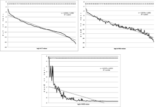
What Is Globalisation?

The KOF Globalisation Index – revisited

Review of the gravity model: origins and critical analysis of its theoretical development

We refer to the fact that: i) the number of countries considered for the GDP per capita is higher (193) than the number of countries considered for exports and imports (179), ii) the result of the former is not separated from the two latter variables, and iii) we have no indications concerning how the time series was built, especially in consideration of the disintegration of the USSR, the unification of Germany, and other major events (see Appendix for our choices in this regard).

All these methodological choices are discussed in detail in the next section.

Intuitively, it can be understood that CT corresponds to weighted Dc. We make this clearer in methodological section.

The size of the latter group varies over the three periods, according to the growing size of WTW. We used the size and features of the WTW to know the criteria and to build groups, see the methodological section. See Appendix for details on the exact composition of each group in each period.

However, as we discuss in methodological section, there is a remarkable difference between BDc and LD, because the former grows linearly, while the latter grows squarely, according to the number of neighbors.

The countries of each segment are listed in Tables 8 , 9 and 10 of Appendix, and some of the many geo-political changes are mentioned.

NEDDI (Network-Based Euclidean Distance) is a software that was made in Python by one of our group members to calculate the relative ED of weighted networks. UCINET in fact only calculates it in absolute terms, and this prevents inter-period and inter-group comparisons. The normalization of weighted ED is anything but simple, and it is not “light” in computational terms.

In the mathematical jargon of network analysis, WDc is called the strength of a node and corresponds to the sum of the weights in the links adjacent to it.

If we indicate the number of neighbors with m, the normalized term is the usual m(m-1) expression.

It would be too long to present details of the algorithm, which implies a somewhat heavy computational load. This aspect and its complexity are perhaps because the software packages with which we are familiar – Ucinet, ORA, R – only provide ED in absolute values. However, we needed to express ED in relative (weighted) terms to express convergence in terms of degree, and to allow its comparisons across the three-time series and different indexes. It should be pointed out that, to achieve such a goal, we set up a dedicated software, NEDDI (Network-Based Euclidean Distance). However, as we explain in the text, after all this work, we discovered that the double operation of standardization and normalization, as well as the high skewness and high range of variance of values made the weighted ED useless.

To be completely sure, we also applied the mathematical relation, and the trends and regression results coincided with those of the binary ED.

Unfortunately, the algorithm for the weighted version of JM is not available.

We used our variables as dependent and independent variables because of the possibility of transforming ? such variables? into panels via the tsset STATA command https://www.stata.com/manuals13/tstsset.pdf .

We also tried the alternative approaches by standardizing CT and WED, and the results were very different from the absolute value case. It is extremely rare to face a problem that is well-known to other researchers who worked on WTW with variables that scale 13 orders of magnitude.

We only show the comparison for one year, but we also conducted such a comparison for the two other possible years, according to the analyses made by the authors, adopting the core-periphery categorization.

This is binary counting: we obtain 1 if a given country of a given group is present in both orderings, otherwise 0. The result was then normalized according to the class size.

It is not surprising that the combination of CD, disaggregated per exports and imports – which means by rows and columns – is rather different than that calculated separately, because the matrix is not symmetrical to the diagonal. Moreover, rows and columns can move in different ways: they can be poorly associated. This is what has happened in our case, as the correlation analysis below shows.

Interestingly, the greatest distances between E20 and the other groups are observed during the second period, which is considered the golden age of globalization.

It should be noted that R 2 is very low in all cases.

For a recent and broad introduction and discussion on the triadic closure principle, homophily and its implications on social and economic networks, see Easley & Kleinberg ( 2010 ).

Abate A, De Benedictis L, Fagiolo G, Tajoli L (2018) Distance-varying assortativity and clustering of the international trade network. Network Science 6:517–544

Article Google Scholar

Abhijeet P (2016) Dependency theory. In: Mackenzie J (ed) The encyclopedia of empire. Wiley, New York

Google Scholar

Alcidi C (2019) Economic integration and income convergence in the EU. Rev Eur Econ Policy 54(1):5–11

Almog A, Squartini T, Garlaschelli D (2017) The double role of GDP in shaping the structure of the international trade network. Int J Comput Econ 7(4):381–398

Armstrong H, Taylor J (2000) Regional economics and policy. Blackwell, Oxford

Austin KF, McKinney LA, Kick EL (2012) Globalization: theories of convergence and divergence in the world-system. In: Babones SJ, Chase-Dunn C (eds) Routledge handbook of world-systems analysis. Taylor and Francis, London

Babones SJ, Chase-Dunn C (eds) (2012) Routledge handbook of world-systems analysis (Routledge international handbooks). Taylor and Francis, London

Backus D, Kehoe PJ, Kydland FE (1992) International real business cycles. J Polit Econ 100(4):745–775

Barabási AL (2016) Network science. Cambridge UP, Cambridge

Barro RJ, Sala–i–Martin X (1992) Convergence. J Polit Econ 100(2):223–251

Barro RJ, Sala-i-Martin X (2004) Economic growth. MIT Press, Cambridge (MA)

De Benedictis L, Nenci S, Santoni G, Tajoli L, Vicarelli C (2013) Network analysis of world trade using the BACI-CEPII dataset. CEPII Working Paper.

Berry H, Guillén MF, Hendi AF (2014) Is there convergence across countries? A spatial approach. J Int Bus Stud 45(4):387–404

Biggiero L (2016) Network analysis for economics and management studies. In: Biggiero L et al (eds) Relational methodologies and epistemology in economics and management sciences. IGI Global, Hershey, pp 1–60

Chapter Google Scholar

Biggiero L, Magnuszewski R (2021) The general ownership structure of the European aerospace industry: a statistical and network analysis. Adv Complex Syst. https://doi.org/10.1142/S0219525921300012

Biggiero L, Angelini PP (2015) Hunting scale-free properties in R&D collaboration networks: Self-organisation, power-law, and policy issues in the European aerospace research area. Technol Forecast Soc Chang 94:21–43

Boschma RA (2005) Proximity and innovation: a critical assessment. Reg Stud 39(1):61–75

Boschma RA, Frenken K (2006) Why is economic geography not an evolutionary science? Towards an evolutionary economic geography. Rev Region Res 23:183–200

Boschma RA, Lambooy JG (1999) Evolutionary economics and economic geography. J Evol Econ 9:411–429

Boschma R, Martin R (2010) The aims and scope of evolutionary economic geography. In: Boschma R, Martin R (eds) The Handbook of evolutionary economic geography. Edward Elgar, Cheltenham (UK), pp 3–42

Brecher R, Choudhri I (1993) Some empirical support for the Heckscher-Ohlin model of production. Can J Econ 26(2):272–285

Caldarelli G (2007) Scale-free networks: complex webs in nature and technology. Oxford UP, NY

Book Google Scholar

Carolan T, Singh N, Talati C (1998) The composition of US-East Asia trade and changing comparative advantage. J Dev Econ 57:361–389

Carter CA, Xianghong L (2004) Changing trade patterns in major OECD countries. Appl Econ 36:1501–1511

Cepeda-López F, Gamboa-Estrada F, León C, Rincón-Castro H (2018) The evolution of world trade from 1995 to 2014: a network approach. J Int Trade Econ Dev. https://doi.org/10.1080/09638199.2018.1549588

Chase-Dunn C, Grimes P (1995) World-systems analysis. Ann Rev Sociol 21:387–417

Chase-Dunn C, Kawano Y, Brewer B (2000) Trade globalization since 1975: waves of integration in the world-system. Am Sociol Rev 65(1):77–95

Coe NM, Dicken P, Hess M (2008a) Global production networks: debates and challenges. J Econ Geogr 8:267–269

Coe NM, Dicken P, Hess M (2008b) Global production networks: realizing the potential. J Econ Geogr 8:271–295

Cotsomitis J, DeBresson C, Kwan A (1991) A re-examination of the technology gap theory of trade: some evidence from time series data for OECD countries. Weltwirtschaftliches Arch 127(4):792–799

Crespo N, Fontoura MP (2007) Integration of CEECs into EU market: structural change and convergence. J Common Market Studies 45(3):611–632

De Bendictis L, Tajoli L (2011) The world trade network. World Econ. https://doi.org/10.1111/j.1467-9701.2011.01360.x

Dueñas M, Fagiolo G (2013) Modelling the international-trade network: a gravity approach. J Econ Interac Coord 8:155–178

Durlauf SN (1996) On the convergence and divergence of growth rates. Econ J 106(437):1016–1018

Easley D, Kleinberg J (2010) Networks, crowds, and markets: reasoning about a highly connected world. Cambridge UP, Cambridge

Fagiolo G, Reyes J, Schiavo S (2010) The evolution of the world trade web: a weighted-network analysis. J Evol Econ 20:479–514

Fagiolo G, Reyes J, Schiavo S (2014) The world-trade web: Topological properties, dynamics, and evolution. HAL Id: hal-01066180. https://hal-sciencespo.archives-ouvertes.fr/hal-01066180 .

Fujita M, Thisse J-F (2002) The economics of agglomeration. Cambridge UP, Cambridge

Fujita M, Krugman P, Venables AJ (1999) The spatial economy: cities, regions, and international trade. MIT Press, Cambridge (MA)

Gagnon JE, Rose AK (1995) Dynamic persistence of industry trade balances: how pervasive is the product cycle? Oxf Econ Pap 47:229–248

García-Pérez G, Boguña M, Allard A, Serrano MA (2016) The hidden hyperbolic geometry of international trade: World Trade Atlas 1870–2013. Sci Rep 6:33441

Guerini, M., Thi Luu, D. & Napoletano, M. (2019). Synchronization patterns in the European Union. halshs-02375416.

Hanneman RA, Riddle M (2005) Introduction to social network methods. University of California, Riverside, Riverside (CA)

Hopkins TK, Wallerstein I (2016) Structural transformations of the world-economy. Review (fernand Braudel Centre) 39(1/4):171–194

Kali R, Reyes J (2007) The architecture of globalization. A network approach to international economic integration. J Int Bus Studies 38(4):595–620

Kick EL, McKinney LA, McDonald S (2011) A multiple-network analysis of the world system of nations. In: Scott J, Carrington PJ (eds) The Sage handbook of social network analysis. Sage, Singapore, pp 1995–1999

Koopman SJ, Azevedo JV (2008) Measuring synchronization and convergence of business cycles for the euro area, UK, and US. Oxford Bull Econ Stat 70(1):23–51

Kose MA, Prasad ES, Terrones ME (2003a) How does globalization affect the synchronization of business cycles? Am Econ Rev 93(2):57–62

Kose MA, Otrok C, Whiteman CH (2003) International business cycles: World, region, and country-specific factors. Am Econ Rev 93(4):1216–1239

Kose MA, Otrok C, Whiteman CH (2008) Understanding the evolution of world business cycles. J Int Econ 75(1):110–130

Kose MA, Otrok C, Pradas E (2012) Global business cycles: convergence or decoupling? Int Econ Rev 53(2):511–538

Krugman P (1991) Geography and trade. MIT Press, Cambridge (MA)

Krugman P (1995) Development, geography, and economic theory. MIT Press, London

Krugman P, Venables AJ (1995) Globalization and the inequality of nations. Quart J Econ 110(4):857–880

Lopes AM, Tenreiro Machado JA, Huffstot JS, Mata ME (2018) Dynamical analysis of the global business-cycle synchronization. PLoS ONE. 13(2):e0191491

Lutz JM, Kihl YW (1990) The NICs, shifting comparative advantage, and the product life cycle. J World Trade 24(1):113–134

Mahutga MC (2006) The persistence of structural inequality? A network analysis of international trade 1965–2000. Soc Forces 84(4):1864–1889

Mancusi ML (2001) Technological specialization in industrial countries: patterns and dynamics. Weltwirtschaftliches Archiv 137(4):593–621

Manning P, Gills BK (eds) (2013) Andre Gunder Frank and global development: visions, remembrances, and explorations. Routledge, London

Maoz Z (2011) Networks of nations: the evolution, structure, and impact of international networks, 1816–2001. Cambridge UP, Cambridge

Martin R, Sunley P (1996) Paul Krugman’s “Geographical Economics” and its implications for regional development theory: a critical assessment. Econ Geogr 72(3):259–292

Martin R, Sunley P (1998) Slow convergence? Post-neoclassical endogenous growth theory and regional development. Econ Geogr 74:201–227

Meyer JW (2000) Globalization: sources and effects on national states and societies. Int Sociol 15:233–248

Monfort P (2008) Convergence of EU regions: Measures and evolution. Working Papers of EU.

Newman MEJ (2010) Introduction to networks. Oxford UP, Oxford

Quah DT (1993) Galton’s fallacy and tests of the convergence hypothesis. Scand J Econ 95(4):427–443

Quah DT (1996) Empirics for economic growth and convergence. Eur Econ Rev 40:1353–1375

Reyes J, Garcia M, Lattimore R (2009) The international economic order and trade architecture. Spat Econ Anal 4(1):73–102

Ritzer G (ed) (2007) The blackwell companion to globalization. Blackwell, Oxford (UK)

Sammarra A, Biggiero L (2008) Heterogeneity and specificity of inter-firm knowledge flows in innovation networks. J Manage Stud 45(4):800–829

Sengupta J (2011) Understanding economic growth: modern theory and experience. Springer, NY

Serrano MA, Garlaschelli D, Boguña M, Loffredo MI (2010) The world trade web: structure, evolution, and modelling, complex networks, encyclopedia of life support systems (EOLSS). EOLSS Publishers, Oxford, UK

Serrano, M. A., Boguñá, M., (2003). Phys. Rev. E 68, 015101(R) (2003).

Smith T (1979) The underdevelopment of development literature: the case of dependency theory. World Politics 31(2):247–288

Smith DA, White DR (1992) Structure and dynamics of the global economy: network analysis of international trade 1965–1980. Soc Forces 70(4):857–893

Snyder D, Kick EL (1979) Structural position in the world system and economic growth, 1955–1970: a multiple-network analysis of transnational interactions. Am J Sociol 84(5):1096–1126

So AY (1999) Social change and development: modernization, dependency, and world-systems theories. Sage Pub, Newbury Park (CA)

Stanistic N (2013) Convergence between the business cycles of Central and Eastern European countries and the Euro area. Baltic J Econ 13(1):63–74

Stehrer R, Wörz J (2003) Technological convergence and trade patterns. Rev World Econ 139(2):192–219

Van Rossem R (1996) The world-system paradigm as general theory of development: a cross-national test. Am Sociol Rev 61:508–527

Van Hamme G, Pion G (2012) The relevance of the world-system approach in the era of globalization of economic flows and networks. Geografiska Annaler Series B, Human Geography. 94(1):65–82

Wallerstein IM (2000) Globalization or the age of transition? Int Sociol 15(2):249–265

Wallerstein IM (2004) World-systems analysis: an introduction. Durham, North Carolina: Duke UP

Wasserman S, Faust K (1994) Social network analysis: methods and applications. Cambridge UP, NY

Williamson JG (1996) Globalization, convergence, and history. J Econ History 56(2):277–306

Download references

Author information

Authors and affiliations.

Department of Industrial Engineering, Information and Economics, University of L’Aquila, Via G. Mezzanotte s.n., Località Acquasanta, 67100, L’Aquila, Italy

Lucio Biggiero

Department of Business and Management, LUISS University (IT), Roma, Italy

Roberto Urbani

You can also search for this author in PubMed Google Scholar

Corresponding author

Correspondence to Roberto Urbani .

Additional information

Publisher's note.

Springer Nature remains neutral with regard to jurisdictional claims in published maps and institutional affiliations.

See Tables See Tables 8 , 9 , 10 , 11 , 12 , 13 , 14 , 15 , 16 , 17 , 18 , 19 , 20 , 21 , 22 , 23 , 24 , 25 , 26 , 27 , 28 , 29 and 30 .

1.1 Criteria to segment time series

Considering that our time series starts in 1980 and finishes in 2016, the rationales that led us to distinguish three periods are the following:

USSR disaggregation, from which 15 new nations (additional nodes for our network) are born: Armenia, Azerbaijan, Belarus, Estonia, Georgia, Kazakhstan, Kyrgyz, Latvia, Lithuania, Moldova, Tajikistan, Turkmenistan, Ukraine, Uzbekistan, plus Russian Federation. It resulted in a 10% size growth of WTW, with a consequent impact also on its trade patterns. These geopolitical changes played an important role in economic growth in the first period because they prepared the ground for the great growth of the golden age of globalization. Further, the signing of free trade agreements between the great world powers such as the 1992 NAFTA between the USA, Canada and Mexico played an important role. Even in the European continent, free trade agreements played a key role as a result of the fall of the USSR. One is the CEFTA (Central European Free Trade Agreement) stipulated in 1992, one year after the official disaggregation of the USSR among many of the countries that were previously part of it. For Western Europe the most important agreement is undoubtedly the TUE (Treaty of Maastricht) signed in 1992 and recognized as the founding treaty of the European Union together with the Treaty of Rome of 1957. The TEU set the political rules and parameters economic and social needs for the entry of the various member states in the European Union. Therefore, the first period ends the year after USSR dissolution;

2007/2008 crisis, which was caused by the mortgage default caused by mortgages passed to history as "subprime" and "near-prime" mortgages. All the sectors of the economy, including the real one, were affected by the financial shock. The relationship between trade in goods and GDP fell sharply in 2009 after the economic crisis, an equally strong rise was in 2010–2011 but already from 2012 began a new gradual decrease until 2014, and then plunged back into significant way in 2015. Also, in 2009 there was a sharp decline in world commodity prices. This had a significant impact on the value of global trade in goods and then rebounded in the opposite direction already in the following year in 2010, at the end of which a decrease began and finally a new significant decline in 2015, a new negative record, arrived at half of the negative value reached in 2009. Another significant indicator that shows the non-stability of world trade in this period is the value of trade in goods and services, this also collapsed in 2009 and then slowly rise above pre-crisis levels in the 2014 and undergo a new crash in 2015 (WTO World Trade Statistical Review, 2016).

The effects of applying these criteria are the segmentation of the 37 years into the following three periods:

1st period 1980–1992, which is composed by 164 nations by aggregating the values of the ones that formed the USSR up to 1991, keeping Yemen united instead of separating and Germany united with GDR;

2 nd period 1993–2007, which is made of 179 nations, obtained by keeping united Serbia and Montenegro, South Africa Custom Union (SACCA) and South Africa, France with Guadeloupe, Martinique, French Guiana and Réunion and the Netherlands Antilles with Aruba;

3rd period 2008–2016, where there are 183 countries and it was not necessary to make separations or unions of countries. This is, in fact, the less “manipulated” set of countries among the three under study.

Rights and permissions

Reprints and permissions

About this article

Biggiero, L., Urbani, R. Testing the convergence hypothesis: a longitudinal and cross-sectional analysis of the world trade web through social network and statistical analyses. J Econ Interact Coord 17 , 713–777 (2022). https://doi.org/10.1007/s11403-021-00341-6

Download citation

Received : 20 March 2019

Accepted : 20 November 2021

Published : 26 December 2021

Issue Date : July 2022

DOI : https://doi.org/10.1007/s11403-021-00341-6

Share this article

Anyone you share the following link with will be able to read this content:

Sorry, a shareable link is not currently available for this article.

Provided by the Springer Nature SharedIt content-sharing initiative

Business cycle synchronization
Convergence hypothesis
Globalization
International trade network
Structural equivalence
World-system theory

JEL Classification

Find a journal
Publish with us
Track your research

IMAGES

The Convergence Hypothesis: Types and Paths
Convergence Theory: 10 Examples and Definition (2024)
The Convergence Hypothesis in Environmental Ethics
PPT
13 Different Types of Hypothesis (2024)
Convergence Hypotheses

VIDEO

Convergence Hypothesis
Mod-01 Lec-06
Synapses3 Convergence, divergence, all or none principle
What is Convergence? Instruments are used to measure Convergence
5.1
The Convergence Hypothesis in Environmental Ethics

COMMENTS

The convergence hypothesis
The debate over catch-up growth—what economists have dubbed the convergence hypothesis —has a long history. The authors choose to focus on research published over the last 30 years. In this recent research, capital, technology, and productivity have been at the root of most understandings of economic growth and convergence.
The Convergence Hypothesis: History, Theory, and Evidence
The hypothesis that per capita output converges across economies over time represents one of the oldest controversies in economics. This essay surveys the history and development of the hypothesis, focusing particularly on its vast literature since the mid-1980s. A summary of empirical analyses, econometric issues, and various tests of the convergence hypothesis are also presented. Moreover ...
PDF The Convergence Hypothesis: History, Theory, and Evidence
The sources of convergence. Abramovitz and David (1996: 21) provide a succinct definition of the conver-gence hypothesis, "Under certain conditions, being behind gives a productivity laggard the ability to grow faster than the early leader. This is the main con-tention of the 'convergence hypothesis'.''.
The convergence hypothesis: History, theory, and evidence
The sources of convergence Abramovitz and David (1996: 21) provide a succinct definition of the convergence hypothesis, " Under certain conditions, being behind gives a productivity laggard the ability to grow faster than the early leader. This is the main contention of the 'convergence hypothesis'.''.
PDF Convergence?: Inferences from Theoretical Models
The convergence hypothesis has been the subject of intense controversy in the past few years. The controversy has been largely empirical, focusing primarily on the validity of ... ical studies based on cross-country regressions (e.g., Barro (1991)) and the evolution of the distribution of income across nations (e.g., Quah (1996)).5 Ironically ...
Growth Theories and Convergence Hypothesis
The element of difference in convergence hypothesis is the distance from the steady state, which is, in neoclassical sense, changing over time and over considered economies. ... diminishing marginal returns and hence higher growth rates of the weaker players potentially constitute a framework for convergence in various agent-based theories. In ...
A test of the convergence hypothesis: the OECD experience, 1950-1990
The convergence hypothesis is based on three main theories [10]: 1—Technology transfer, 2—Neoclassical growth model and 3—Olson's thesis. The technology transfer argument asserts that the flow of technology creates a tendency for poor countries to converge toward the rich ones [11].
1 Convergence Theory
Convergence theory is the idea that as rich countries got richer, they developed similar economic, political, and social structures and to some extent common values and beliefs. The driving force that moves modern societies toward common structures and cultures is continuing industrialization. ... This convergence argument—based on theory and ...
Convergence (economics)
The idea of convergence in economics (also sometimes known as the catch-up effect) is the hypothesis that poorer economies' per capita incomes will tend to grow at faster rates than richer economies. In the Solow-Swan growth model, economic growth is driven by the accumulation of physical capital until this optimum level of capital per worker, which is the "steady state" is reached, where ...
Convergence? Inferences from Theoretical Models
convergence hypothesis and the club convergence hypothesis. Furthermore, inclusion of empirically significant variables such as human capital, income distribution, and fertility, in conventional growth models, along with capital ... hypothesis has been refuted in recent empirical studies based on cross-country regressions (e.g. Barro (1991 ...
20.4 Economic Convergence
Some low-income and middle-income economies around the world have shown a pattern of convergence, in which their economies grow faster than those of high-income countries. GDP increased by an average rate of 2.7% per year in the 1990s and 1.7% per year from 2010 to 2019 in the high-income countries of the world, which include the United States ...
The Convergence Hypothesis: History, Theory, and Evidence
The hypothesis that per capita output converges across economies over time represents one of the oldest controversies in economics. This essay surveys the history and development of the hypothesis, focusing particularly on its vast literature since the mid-1980s. A summary of empirical analyses, econometric issues, and various tests of the convergence hypothesis are also presented.
Convergence hypothesis
The theory that socialism and capitalism will, over time, become increasingly alike in economic and social terms. Convergence theory was popular in the 1950s and 1960s, when Raymond Aron, John ... From: convergence hypothesis in Dictionary of the Social Sciences ». Subjects: Social sciences.
20.4 Economic Convergence
20.4 Economic Convergence. By the end of this section, you will be able to: Some low-income and middle-income economies around the world have shown a pattern of convergence, in which their economies grow faster than those of high-income countries. GDP increased by an average rate of 2.7% per year in the 1990s and 2.3% per year from 2000 to 2008 ...
Convergence: Theory, Econometrics, and Empirics
In Schumpeterian growth theory convergence occurs through productivity by means of technology transfer as well as through capital accumulation (Aghion and Howitt 2009). Here, the focus will lie on the productivity effects. ... The time-series concept however features a stricter notion of convergence than those based on cross-section regressions ...
Convergence Theory
Convergence theory is an economic theory that presupposes that the concept of development is. defined by economic growth. It frames convergence with supposedly "developed" nations as a goal of so-called "undeveloped" or "developing" nations, and in doing so, fails to account for the numerous negative outcomes that often follow this economically ...
Convergence hypothesis: a systematic literature review with
The study presents a systematic literature review with bibliometric analysis of the existing literature on convergence hypothesis sourced from the Scopus database over two decades spanning 2000 to 2020. Literature review based on year, source, affiliation, country, and contributing authors is done, along with bibliographic coupling, thematic evaluation and content analysis. Findings suggest ...
The Catch-Up Effect Definition and Theory of Convergence
Catch-Up Effect: The catch-up effect is a theory speculating that poorer economies will tend to grow more rapidly than wealthier economies, and so all economies in time will converge in terms of ...
Convergence Theories
CONVERGENCE THEORIESThe idea that societies move toward a condition of similarity—that they converge in one or more respects—is a common feature of various theories of social change. The notion that differences among societies will decrease over time can be found in many works of eighteenth and nineteenth century social thinkers, from the prerevolutionary French philosophes and the ...
PDF Chapter 4 Convergence: Theory, Econometrics, and Empirics
Convergence: Theory, Econometrics, and Empirics 4.1 Models of Economic Growth and Convergence ... workings is based on the textbooks of economic growth by Aghion and Howitt (2009), Barro and Sala-i-Martin (1995, 2004), Frenkel and Hemmer (1999), as well as Romer (2005). A simpliﬁed version of the Solow-Swan model is described
Contextualism and Norton's Convergence Hypothesis
Convergence in Environmental Values: An Empirical and Conceptual Defense. Bryan Norton's convergence hypothesis, which predicts that nonanthropocentric and human-based philosophical positions will actually converge on long-sighted, multi-value environmental policy, has…. The Transformative value of Ecological Pragmatism.
IBUS 330 ch4 Flashcards
Study with Quizlet and memorize flashcards containing terms like The GLOBE instrument addresses the idea that a leader's effectiveness is, The convergence hypothesis refers to a universal acceptance of Blank______ across cultures., The convergence hypothesis is based on the idea that and more.
MISATO: machine learning dataset of protein-ligand complexes for
MISATO is a database for structure-based drug discovery that combines quantum mechanics data with molecular dynamics simulations on ~20,000 protein-ligand structures. ... theory. Reinspection of ...
Testing the convergence hypothesis: a longitudinal and cross ...
We test the convergence hypothesis in two directions: the level and trend of convergence, and its possible determination by means of structural or economic globalization, measured in terms of exchanges density and economic values, respectively. ... The hypotheses based on the former line of reasoning are easy to define, because it is sufficient ...
Land
The speed of regional convergence from fastest to slowest was central > west > east, with the absolute convergence speeds of 0.0505, 0.0360, and 0.0212, respectively. Finally, policy recommendations are proposed to achieve regional carbon neutrality for the PPRD. ... Based on the Difference in Land Use Carbon Budget" Land 13, no. 5: 634. https ...

This website uses cookies.

The convergence hypothesis

Are poor countries catching up with rich countries?

The Great Divergence

Can pathogen concentrations explain which countries developed sooner?

The convergence hypothesis: History, theory, and evidence

Related Papers

RELATED PAPERS

RELATED TOPICS

1 Convergence Theory

Signed in as

Personal account

Institutional access

IP based access

Sign in through your institution

Sign in with a library card

Society Members

Sign in through society site

Sign in using a personal account

Viewing your signed in accounts

Signed in but can't access content

This Feature Is Available To Subscribers Only

20.4 Economic Convergence

Arguments Favoring Convergence

Arguments That Convergence Is neither Inevitable nor Likely

The Slowness of Convergence

Bring It Home

Recently viewed (0)

Related Content

More Like This

convergence hypothesis

Related content in Oxford Reference

20.4 Economic Convergence

Arguments Favoring Convergence

Arguments That Convergence Is neither Inevitable nor Likely

The Slowness of Convergence

Calories and Economic Growth

Key Concepts and Summary

Self-Check Questions

Review Questions

Critical Thinking Questions

What Is Convergence Theory?

Convergence vs. Divergence

Sociological Critiques

What Is the Catch-Up Effect?

The Bottom Line

The Catch-Up Effect Definition and Theory of Convergence

Key Takeaways

Understanding the Catch-Up Effect

Limitations to the Catch-Up Effect

Lack of Social Capabilities

Lack of Open Trade

Population Growth

Example of the Catch-Up Effect

How Can Underdeveloped Countries Benefit From the Catch-Up Effect?

Has Globalization Made the Catch-Up Effect More Prevalent?

Why Does the Catch-Up Effect Diminish for Industrialized Countries?

MISATO: machine learning dataset of protein–ligand complexes for structure-based drug discovery

Similar content being viewed by others

Accurate structure prediction of biomolecular interactions with AlphaFold 3

Highly accurate protein structure prediction with AlphaFold

De novo generation of multi-target compounds using deep generative chemistry

MISATO dataset

Source data

Typical limitations in structural datasets

Evaluation of the QM-based ligand curation

QM-derived properties

MD simulations

Experimental validation

Binding affinity benchmark and validation

Semi-empirical calculations

QM curation of ligand space

Access to the database

AI applications

Scoring of ligands with AutoDock Vina

Correlation with experimental B factors

Binding affinity benchmark

Protein purification and NMR spectroscopy

Statistics and reproducibility

Reporting summary