null hypothesis genetics example

Statistics Made Easy

How to Write a Null Hypothesis (5 Examples)

A hypothesis test uses sample data to determine whether or not some claim about a population parameter is true.

Whenever we perform a hypothesis test, we always write a null hypothesis and an alternative hypothesis, which take the following forms:

H 0 (Null Hypothesis): Population parameter =,  ≤, ≥ some value

H A  (Alternative Hypothesis): Population parameter <, >, ≠ some value

Note that the null hypothesis always contains the equal sign .

We interpret the hypotheses as follows:

Null hypothesis: The sample data provides no evidence to support some claim being made by an individual.

Alternative hypothesis: The sample data  does provide sufficient evidence to support the claim being made by an individual.

For example, suppose it’s assumed that the average height of a certain species of plant is 20 inches tall. However, one botanist claims the true average height is greater than 20 inches.

To test this claim, she may go out and collect a random sample of plants. She can then use this sample data to perform a hypothesis test using the following two hypotheses:

H 0 : μ ≤ 20 (the true mean height of plants is equal to or even less than 20 inches)

H A : μ > 20 (the true mean height of plants is greater than 20 inches)

If the sample data gathered by the botanist shows that the mean height of this species of plants is significantly greater than 20 inches, she can reject the null hypothesis and conclude that the mean height is greater than 20 inches.

Read through the following examples to gain a better understanding of how to write a null hypothesis in different situations.

Example 1: Weight of Turtles

A biologist wants to test whether or not the true mean weight of a certain species of turtles is 300 pounds. To test this, he goes out and measures the weight of a random sample of 40 turtles.

Here is how to write the null and alternative hypotheses for this scenario:

H 0 : μ = 300 (the true mean weight is equal to 300 pounds)

H A : μ ≠ 300 (the true mean weight is not equal to 300 pounds)

Example 2: Height of Males

It’s assumed that the mean height of males in a certain city is 68 inches. However, an independent researcher believes the true mean height is greater than 68 inches. To test this, he goes out and collects the height of 50 males in the city.

H 0 : μ ≤ 68 (the true mean height is equal to or even less than 68 inches)

H A : μ > 68 (the true mean height is greater than 68 inches)

Example 3: Graduation Rates

A university states that 80% of all students graduate on time. However, an independent researcher believes that less than 80% of all students graduate on time. To test this, she collects data on the proportion of students who graduated on time last year at the university.

H 0 : p ≥ 0.80 (the true proportion of students who graduate on time is 80% or higher)

H A : μ < 0.80 (the true proportion of students who graduate on time is less than 80%)

Example 4: Burger Weights

A food researcher wants to test whether or not the true mean weight of a burger at a certain restaurant is 7 ounces. To test this, he goes out and measures the weight of a random sample of 20 burgers from this restaurant.

H 0 : μ = 7 (the true mean weight is equal to 7 ounces)

H A : μ ≠ 7 (the true mean weight is not equal to 7 ounces)

Example 5: Citizen Support

A politician claims that less than 30% of citizens in a certain town support a certain law. To test this, he goes out and surveys 200 citizens on whether or not they support the law.

H 0 : p ≥ .30 (the true proportion of citizens who support the law is greater than or equal to 30%)

H A : μ < 0.30 (the true proportion of citizens who support the law is less than 30%)

Additional Resources

Introduction to Hypothesis Testing Introduction to Confidence Intervals An Explanation of P-Values and Statistical Significance

Featured Posts

Hey there. My name is Zach Bobbitt. I have a Masters of Science degree in Applied Statistics and I’ve worked on machine learning algorithms for professional businesses in both healthcare and retail. I’m passionate about statistics, machine learning, and data visualization and I created Statology to be a resource for both students and teachers alike.  My goal with this site is to help you learn statistics through using simple terms, plenty of real-world examples, and helpful illustrations.

2 Replies to “How to Write a Null Hypothesis (5 Examples)”

you are amazing, thank you so much

Say I am a botanist hypothesizing the average height of daisies is 20 inches, or not? Does T = (ave – 20 inches) / √ variance / (80 / 4)? … This assumes 40 real measures + 40 fake = 80 n, but that seems questionable. Please advise.

Leave a Reply Cancel reply

Your email address will not be published. Required fields are marked *

Join the Statology Community

Sign up to receive Statology's exclusive study resource: 100 practice problems with step-by-step solutions. Plus, get our latest insights, tutorials, and data analysis tips straight to your inbox!

By subscribing you accept Statology's Privacy Policy.

AP® Biology

The chi square test: ap® biology crash course.

• The Albert Team
• Last Updated On: March 7, 2024

The statistics section of the AP® Biology exam is without a doubt one of the most notoriously difficult sections. Biology students are comfortable with memorizing and understanding content, which is why this topic seems like the most difficult to master. In this article,  The Chi Square Test: AP® Biology Crash Course , we will teach you a system for how to perform the Chi Square test every time. We will begin by reviewing some topics that you must know about statistics before you can complete the Chi Square test. Next, we will simplify the equation by defining each of the Chi Square variables. We will then use a simple example as practice to make sure that we have learned every part of the equation. Finally, we will finish with reviewing a more difficult question that you could see on your AP® Biology exam .

Null and Alternative Hypotheses

As background information, first you need to understand that a scientist must create the null and alternative hypotheses prior to performing their experiment. If the dependent variable is not influenced by the independent variable , the null hypothesis will be accepted. If the dependent variable is influenced by the independent variable, the data should lead the scientist to reject the null hypothesis . The null and alternative hypotheses can be a difficult topic to describe. Let’s look at an example.

Consider an experiment about flipping a coin. The null hypothesis would be that you would observe the coin landing on heads fifty percent of the time and the coin landing on tails fifty percent of the time. The null hypothesis predicts that you will not see a change in your data due to the independent variable.

The alternative hypothesis for this experiment would be that you would not observe the coins landing on heads and tails an even number of times. You could choose to hypothesize you would see more heads, that you would see more tails, or that you would just see a different ratio than 1:1. Any of these hypotheses would be acceptable as alternative hypotheses.

Defining the Variables

Now we will go over the Chi-Square equation. One of the most difficult parts of learning statistics is the long and confusing equations. In order to master the Chi Square test, we will begin by defining the variables.

This is the Chi Square test equation. You must know how to use this equation for the AP® Bio exam. However, you will not need to memorize the equation; it will be provided to you on the AP® Biology Equations and Formulas sheet that you will receive at the beginning of your examination.

Now that you have seen the equation, let’s define each of the variables so that you can begin to understand it!

•   X 2  :The first variable, which looks like an x, is called chi squared. You can think of chi like x in algebra because it will be the variable that you will solve for during your statistical test. •   ∑ : This symbol is called sigma. Sigma is the symbol that is used to mean “sum” in statistics. In this case, this means that we will be adding everything that comes after the sigma together. •   O : This variable will be the observed data that you record during your experiment. This could be any quantitative data that is collected, such as: height, weight, number of times something occurs, etc. An example of this would be the recorded number of times that you get heads or tails in a coin-flipping experiment. •   E : This variable will be the expected data that you will determine before running your experiment. This will always be the data that you would expect to see if your independent variable does not impact your dependent variable. For example, in the case of coin flips, this would be 50 heads and 50 tails.

The equation should begin to make more sense now that the variables are defined.

Working out the Coin Flip

We have talked about the coin flip example and, now that we know the equation, we will solve the problem. Let’s pretend that we performed the coin flip experiment and got the following data:

Now we put these numbers into the equation:

Heads (55-50) 2 /50= .5

Tails (45-50) 2 /50= .5

Lastly, we add them together.

c 2 = .5+.5=1

Now that we have c 2 we must figure out what that means for our experiment! To do that, we must review one more concept.

Degrees of Freedom and Critical Values

Degrees of freedom is a term that statisticians use to determine what values a scientist must get for the data to be significantly different from the expected values. That may sound confusing, so let’s try and simplify it. In order for a scientist to say that the observed data is different from the expected data, there is a numerical threshold the scientist must reach, which is based on the number of outcomes and a chosen critical value.

Let’s return to our coin flipping example. When we are flipping the coin, there are two outcomes: heads and tails. To get degrees of freedom, we take the number of outcomes and subtract one; therefore, in this experiment, the degree of freedom is one. We then take that information and look at a table to determine our chi-square value:

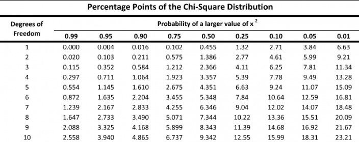
We will look at the column for one degree of freedom. Typically, scientists use a .05 critical value. A .05 critical value represents that there is a 95% chance that the difference between the data you expected to get and the data you observed is due to something other than chance. In this example, our value will be 3.84.

Coin Flip Results

In our coin flip experiment, Chi Square was 1. When we look at the table, we see that Chi Square must have been greater than 3.84 for us to say that the expected data was significantly different from the observed data. We did not reach that threshold. So, for this example, we will say that we failed to reject the null hypothesis.

The best way to get better at these statistical questions is to practice. Next, we will go through a question using the Chi Square Test that you could see on your AP® Bio exam.

AP® Biology Exam Question

This question was adapted from the 2013 AP® Biology exam.

In an investigation of fruit-fly behavior, a covered choice chamber is used to test whether the spatial distribution of flies is affected by the presence of a substance placed at one end of the chamber. To test the flies’ preference for glucose, 60 flies are introduced into the middle of the choice chamber at the insertion point. A ripe banana is placed at one end of the chamber, and an unripe banana is placed at the other end. The positions of flies are observed and recorded after 1 minute and after 10 minutes. Perform a Chi Square test on the data for the ten minute time point. Specify the null hypothesis and accept or reject it.

Okay, we will begin by identifying the null hypothesis . The null hypothesis would be that the flies would be evenly distributed across the three chambers (ripe, middle, and unripe).

Next, we will perform the Chi-Square test just like we did in the heads or tails experiment. Because there are three conditions, it may be helpful to use this set up to organize yourself:

Ok, so we have a Chi Square of 48.9. Our degrees of freedom are 3(ripe, middle, unripe)-1=2. Let’s look at that table above for a confidence variable of .05. You should get a value of 5.99. Our Chi Square value of 48.9 is much larger than 5.99 so in this case we are able to reject the null hypothesis. This means that the flies are not randomly assorting themselves, and the banana is influencing their behavior.

The Chi Square test is something that takes practice. Once you learn the system of solving these problems, you will be able to solve any Chi Square problem using the exact same method every time! In this article, we have reviewed the Chi Square test using two examples. If you are still interested in reviewing the bio-statistics that will be on your AP® Biology Exam, please check out our article The Dihybrid Cross Problem: AP® Biology Crash Course . Let us know how studying is going and if you have any questions!

Need help preparing for your AP® Biology exam?

Albert has hundreds of AP® Biology practice questions, free response, and full-length practice tests to try out.

Interested in a school license?​

Popular posts.

AP® Score Calculators

Simulate how different MCQ and FRQ scores translate into AP® scores

AP® Review Guides

The ultimate review guides for AP® subjects to help you plan and structure your prep.

Core Subject Review Guides

Review the most important topics in Physics and Algebra 1 .

SAT® Score Calculator

See how scores on each section impacts your overall SAT® score

ACT® Score Calculator

See how scores on each section impacts your overall ACT® score

Grammar Review Hub

Comprehensive review of grammar skills

AP® Posters

Download updated posters summarizing the main topics and structure for each AP® exam.

This page has been archived and is no longer updated

Neutral Theory: The Null Hypothesis of Molecular Evolution

The evolution of living organisms is the consequence of two processes. First, evolution depends on the genetic variability generated by mutations , which continuously arise within populations. Second, it also relies on changes in the frequency of alleles within populations over time.

The fate of those mutations that affect the fitness of their carrier is partly determined by natural selection . On one hand, new alleles that confer a higher fitness tend to increase in frequency over time until they reach fixation, thus replacing the ancestral allele in the population . This evolutionary process is called positive or directional selectio n . Conversely, new mutations that decrease the carrier's fitness tend to disappear from populations through a process known as negative or purifying selection . Finally, it may happen that a mutation is advantageous only in heterozygotes but not in homozygotes. Such alleles tend to be maintained at an intermediate frequency in populations by way of the process known as balancing selection .

However, natural selection is not the only factor that can lead to changes in allele frequency. For example, consider a theoretical population in which all individuals, or genotypes, have exactly the same fitness. In this situation, natural selection does not operate, because all genotypes have the same chance to contribute to the next generation. Given that populations do not grow infinitely and that each individual produces many gametes , it follows that only a fraction of the gametes that are produced will succeed in developing into adults. Thus, in each generation, allelic frequencies may change simply as a consequence of this random process of gamete sampling. This process is called genetic drift . The difference between genetic drift and natural selection is that changes in allele frequency caused by genetic drift are random, rather than directional. Ultimately, genetic drift leads to the fixation of some alleles and the loss of others.

But what about mutations that do not affect the fitness of individuals? These so-called neutral mutations are not affected by natural selection and, hence, their fate is essentially driven by genetic drift. Interestingly, Darwin himself recognized that some traits might evolve without being affected by natural selection:

" Variations neither useful nor injurious would not be affected by natural selection, and would be left either a fluctuating element, as perhaps we see in certain polymorphic species , or would ultimately become fixed , owing to the nature of the organism and the nature of the conditions. " (Darwin, 1859)

It is important to note, however, that the impact of genetic drift is not limited to neutral mutations. Because of genetic drift, most advantageous mutations are eventually lost, whereas some weakly deleterious mutations may become fixed.

Beyond selection and drift, biased gene conversion (BGC) is a third process that can cause changes in allele frequency in sexual populations. BGC is linked to meiotic crossing-over . When crossing-over occurs between two homologous chromosomes, the intermediate includes heteroduplex DNA—a region in which one DNA strand is from one homologue and the other strand is from the other homologue. Regardless of the ultimate resolution of the crossover intermediate (in other words, whether the regions on either side of the crossover junction recombine), base-pairing mismatches in the heteroduplex region must be resolved. As a consequence, when a given locus resides in the heteroduplex region, one allele can be "copied and pasted" onto the other one during gene conversion .

BGC is said to be biased if one allele has a higher probability of conversion than the other. In that situation, the donor allele will occur at higher frequency in the gamete pool than the converted allele. Hence, BGC tends to increase the frequency of such donor alleles within populations. There is evidence that BGC occurs in many eukaryotic species, and various observations suggest that it might result from a bias in the repair of DNA mismatches in the heteroduplex DNA formed during recombination (Marais, 2003). Again, it is important to note that the impact of BGC is not limited to the evolution of neutral mutations: BGC can favor the fixation of donor alleles even if these alleles are weakly deleterious (Galtier & Duret, 2007).

The Selectionist vs. Neutralist Controversy

Until the 1960s, the prevailing view was that natural selection played a dominant role. According to this view, differences between species were thought to consist mainly of mutations that had been fixed by positive selection—mutations that contributed to the adaptation of a species to its environment . In contrast, the existing polymorphism within populations was thought to reflect balancing selection. Thus, according to this so-called selectionist theory, nonadaptive processes were at best minor contributors to evolution. However, the analysis of sequence data that became available in the late 1960s considerably challenged this view. In 1968, these empirical data and new theoretical developments led Motoo Kimura to propose a new hypothesis, now known as the neutral theory of molecular evolution (Kimura, 1968). Kimura subsequently summarized his theory as follows:

"This neutral theory claims that the overwhelming majority of evolutionary changes at the molecular level are not caused by selection acting on advantageous mutants, but by random fixation of selectively neutral or very nearly neutral mutants through the cumulative effect of sampling drift (due to finite population number) under continued input of new mutations" (Kimura, 1991)

Immediately, this theory caused controversy and gave rise to opposition from many evolutionary biologists. However, the theory also made several strong predictions that could be tested against actual data. Notably, if most of the sequence divergence between species is due to neutral evolution, then one should expect more changes in functionally less important sequences. When Kimura proposed the neutral theory in 1968, only a few protein sequences were available. By the 1980s, however, the much larger amount of DNA sequence data that had accumulated largely validated this prediction. In fact, in light of these new sequence data, Kimura himself published a review of his theory in 1991. In his paper, he pointed out several important observations that had been recently reported, including the following:

• In protein sequences, conservative changes—substitutions of amino acids that have similar biochemical properties and are therefore less likely to affect the function of a protein—occur much more frequently than radical changes.
• Synonymous base substitutions (i.e., those that do not cause amino acid changes) occur almost always at a much higher rate than nonsynonymous substitutions.
• Noncoding sequences, such as introns, evolve at a high rate similar to that of synonymous sites.
• Pseudogenes, or dead genes, evolve at a high rate, and this rate is about the same in three-codon positions.

All of these observations have been widely confirmed with the genomic data that are now available (Figure 1). These observations are consistent with the neutral theory but contradict selectionist theory. After all, if most substitutions were adaptive, as argued by selectionist theory, one would expect fewer substitutions in DNA regions where changes have little or no effect on phenotype (e.g., pseudogenes, noncoding sequences, synonymous sites) than in functionally important regions.

It must be stressed that the neutral theory of molecular evolution is not an anti-Darwinian theory. Both the selectionist and neutral theories recognize that natural selection is responsible for the adaptation of organisms to their environment. Both also recognize that most new mutations in functionally important regions are deleterious and that purifying selection quickly removes these deleterious mutations from populations. Thus, these mutations do not contribute—or contribute very little—to sequence divergence between species and to polymorphisms within species. Rather, the dispute between selectionists and neutralists relates only to the relative proportion of neutral and advantageous mutations that contribute to sequence divergence and polymorphism.

Analysis of genomic sequence data reveals that there is no "all or nothing" answer to this dispute. In fact, the proportion of neutral substitutions varies widely among taxa. However, it is now clearly established that nonadaptive processes cannot be neglected. Even in taxa in which selection is very effective, a large fraction of substitutions are indeed neutral.

Population Size Matters

The classification of mutations into three distinct types—deleterious, neutral, and advantageous—is of course an oversimplification. In reality, there is a continuum from highly deleterious to weakly deleterious, nearly neutral, neutral, weakly advantageous, and strongly advantageous mutations. It is important to note that the effectiveness of selection on a mutation depends both on the fitness effect of this mutation (the selection coefficient s ) and on the effective population size ( N e ). Specifically, when the product N e s is much less than 1, the fate of mutations is essentially determined by random genetic drift. In other words, in small populations, the stochastic effects of random genetic drift overcome the effects of selection. Thus, all mutations for which N e s is much less than 1 can be considered effectively neutral. This implies that the proportion of neutral mutations is expected to inversely vary with a taxon 's effective population size.

Empirical data are consistent with this prediction. For example, in Drosophila species (where N e is about 10 6 ), the proportion of nonsynonymous substitutions that have been fixed by positive selection is about 50%. Contrast this with the data for hominids (with N e around 10,000 to 30,000), where this proportion is close to zero. Similarly, the proportion of nonsynonymous mutations that are effectively neutral is less than 16% in Drosophila, whereas it is about 30% in hominids (Eyre-Walker & Keightley, 2007).

The most important contribution of Kimura's work is that it provides a theoretical framework for developing methods that detect the action of selection within genomes. However, to be able to demonstrate that a sequence is subject to selective pressure , one must reject the null hypothesis that this sequence evolves neutrally. For example, one strong (and elegant) prediction of the neutral theory is that at selectively neutral sites, the rate of substitution is equal to the rate of mutation (Kimura, 1968). To demonstrate this, consider a neutral site: a DNA position at which all alleles are selectively equivalent, and where the rate of mutation per generation is u . In a haploid population of size N , Nu mutations occur at this site at each generation. Given that there is no selection, all genotypes have the same probability to reach fixation. Under a neutral model , the probability that an allele or mutation fixes is simply its relative frequency in the population. For a new mutation in a haploid population, this relative frequency is 1/ N ; thus, the probability that a new mutation reaches fixation is simply 1/ N (the same reasoning also holds for diploid species). The rate of substitution per generation ( K ) is obtained simply by multiplying the number of mutations that occur at each generation by their probability of fixation. Thus, for neutrally evolving sites, the equation becomes the following:

K = Nu × 1/ N = u

Of course, because of natural selection, advantageous mutations have a higher probability of fixation than neutral mutations, and deleterious mutations have a lower probability of fixation. It therefore follows that sequences subject to positive selection evolve faster than neutral sites ( K > u ), whereas sequences subject to negative selection evolve more slowly ( K u ). This simple result is the basis of many tests that have been developed to detect selection. Note, however, that selection is not the only process that can affect K . Indeed, BGC can affect the probability of allele fixation and hence substitution rates, as previously mentioned.

Why Should We Care About Neutral Evolution?

The main goal of biology is to understand how living organisms function and how they adapt to ever-fluctuating environments. So one may wonder why it is important to study neutral evolutionary processes that, a priori , seem to have little effect on the evolution of phenotypes. There are actually three primary reasons for this adjusted focus.

First, as mentioned earlier, the neutral theory is the underlying basis of selection tests. These tests are widely used to identify functional elements (e.g., genes and regulatory regions) within genomic sequences. The basic principle of this comparative genomics approach is that functional elements are subject to selective pressure, and hence their pattern of evolution differs from the neutral expectation. To be able to detect selection, it is therefore necessary to have a good understanding of all the nonadaptive evolutionary processes that affect sequence evolution—mutation, BGC, and genetic drift. Notably, the selection test mentioned above requires knowledge of u . This parameter can be estimated by measuring K in sites that are expected, a priori , to be neutral—pseudogenes or defective transposable elements, for example—although u may vary across chromosomes. Also, in some eukaryotic taxa, BGC appears to have a strong influence on genome evolution by favoring the fixation of AT to GC mutations (Marias, 2003). This BGC drive leads to enrichment of GC-content in genomic regions that feature high crossover rates. Many lines of evidence indicate this process is responsible for the strong regional variations in GC-content across mammalian chromosomes. In mammals, crossovers occur essentially in hot spots (typically 1 to 2 kilobases long), and BGC can create strong substitution hot spots, where the local substitution rate can be up to 20 times higher than in the rest of the genome (Duret & Arndt, 2008). In some cases, BGC may even counteract the action of selection and lead to the fixation of deleterious mutations, which implies that BGC can contribute to species maladaptation. Thus, before concluding that sequences are subject to selection, it is necessary to test whether the observed pattern of sequence evolution cannot be explained by this nonadaptive process (Galtier & Duret, 2007).

A second reason why knowledge of neutral sequence evolution is important is that it provides information about molecular processes that are involved in genome functioning. For example, it has been found that in some taxa, there is an asymmetry of substitution patterns between the two DNA strands. This pattern is caused by the asymmetry of the DNA replication process and can be used to infer the location of replication origins within chromosomes (Lobry, 1996). Similarly, the asymmetry of substitution patterns can be used to detect and orient transcription in the germ line of mammals (Green et al ., 2003). The analysis of neutral substitution patterns also revealed the existence of a homology-dependent mechanism of DNA methylation in primates (Meunier et al ., 2005).

Finally, one point that is often not fully appreciated is that neutral evolution can ultimately contribute to phenotypic evolution and to species adaptation. Kimura noted that many gene duplications may get fixed by random genetic drift, simply because they are not deleterious . Then, because of relaxation of selective pressures, one or both copies may accumulate mutations that otherwise would have been counterselected. Some of these mutants will turn out to be useful for the adaptation of organisms to their environment (Kimura, 1991). The idea that nonadaptive processes may have a major impact on the evolution of biological complexity has been largely developed by Michael Lynch (Lynch, 2006). Following duplication, the functions of the duplicates are initially redundant. Also, most gene products contribute to multiple aspects of an organism's phenotype. If one duplicate undergoes a mutation that knocks out part of its contribution to phenotype, it is released from purifying selection to maintain those functions. The reduction of negative selection efficiency allows a wider exploration of the space of possible genotypes, which may allow for improvements in remaining functions.

Also, regardless of the steps involved, the evolutionary trajectory between one genotype and another better-fit genotype may sometimes have to pass through a less-optimal genotype. Thus, a reduction of effective population size, which increases the effect of random drift, may allow the fixation of weakly deleterious mutations to pass through this less-optimal genotype, and hence can open a new evolutionary trajectory, possibly toward better-adapted genotypes.

References and Recommended Reading

Darwin, C. On the Origin of Species by Means of Natural Selection, or the Preservation of Favoured Races in the Struggle for Life (London, John Murray, 1859)

Duret, L., & Arndt, P. F. The impact of recombination on nucleotide substitutions in the human genome. PLoS Genetics 4 , e1000071 (2008) ( link to article )

Eyre-Walker, A., & Keightley, P. D. The distribution of fitness effects of new mutations. Nature Reviews Genetics 8 , 610–618 (2007) ( link to article )

Galtier, N., & Duret, L. Adaptation or biased gene conversion? Extending the null hypothesis of molecular evolution. Trends in Genetics 23 , 273–277 (2007)

Graur, D., & Li, W. Fundamentals of Molecular Evolution (Sunderland, MA, Sinauer Associates, 2000)

Green, P., et al. Transcription-associated mutational asymmetry in mammalian evolution. Nature Genetics 33 , 514–517 (2003) doi:10.1038/ng1103 ( link to article )

Kimura, M. Evolutionary rate at the molecular level. Nature 217 , 624–626 (1968) doi:10.1038/217624a0 ( link to article )

———. The neutral theory of molecular evolution: A review of recent evidence. Japanese Journal of Genetics 66 , 367–386 (1991)

Lobry, J. R. Asymmetric substitution patterns in the two DNA strands of bacteria. Molecular Biology and Evolution 13 , 660–665 (1996)

Lynch, M. The origins of eukaryotic gene structure. Molecular Biology and Evolution 23 , 450–468 (2006)

———. The Origins of Genome Architecture (Sunderland, MA, Sinauer Associates, 2007)

Makalowski, W., & Boguski, M. S. Evolutionary parameters of the transcribed mammalian genome: An analysis of 2,820 orthologous rodent and human sequences. Proceedings of the National Academy of Sciences 95 , 9407–9412 (1998)

Marais, G. Biased gene conversion: Implications for genome and sex evolution. Trends in Genetics 19 , 330–338 (2003)

Meunier, J., et al . Homology-dependent methylation in primate repetitive DNA. Proceedings of the National Academy of Sciences 102 , 5471–5476 (2005)

• Add Content to Group

Article History

Flag inappropriate.

Email your Friend

•  |  Lead Editor:  Bob Sheehy ,  Norman Johnson

Within this Subject (14)

• Genome Evolution (1)
• Macroevolution (1)
• Microevolution (6)
• Phylogeny (2)
• Speciation (4)

Other Topic Rooms

• Gene Inheritance and Transmission
• Gene Expression and Regulation
• Nucleic Acid Structure and Function
• Chromosomes and Cytogenetics
• Evolutionary Genetics
• Population and Quantitative Genetics
• Genes and Disease
• Genetics and Society
• Cell Origins and Metabolism
• Proteins and Gene Expression
• Subcellular Compartments
• Cell Communication
• Cell Cycle and Cell Division

© 2014 Nature Education

• Press Room |
• Terms of Use |
• Privacy Notice |

Visual Browse

• Toggle navigation

BIO2450L-Genetics; Prof. Christopher Blair

Open educational resources for Genetics

Probability, Statistics, and Measurements

The goal of this laboratory is to provide an introduction to basic concepts and techniques commonly used to study genetics. The first portion of the lab is devoted to the concept of probability and how we can use basic probability theory to understand genetic concepts and crosses . Genetic crosses are commonly used to study patterns of inheritance of traits . A trait, or a character, is generally any observable phenotypic characteristic of an organism such as eye color, skin color, height, etc. Gregor Mendel, often considered the father of genetics, performed many genetic crosses to quantify patterns of inheritance in pea plants. Based on the results of his experiments he came up with three laws:

Law 1: Law of Segregation

Alleles in diploid individuals separate during the process of gamete formation (meiosis).

Remember that a diploid cell contains two sets of chromosomes, one from the father and one from the mother. Thus, each gene will contain two alleles. The alleles can either be the same (homozygous) or different (heterozygous). For example, if we assume that pea pod color (green versus yellow) is controlled by a single gene with two alleles ( R and r ), RR and rr would represent homozygotes and Rr would indicate a heterozygote. During gamete formation, only one of the two alleles will be passed on to the sperm or egg. In other words, the two alleles segregate from one another (see Fig. 1).

  Law 2: Law of Independent Assortment

Different genes randomly sort their alleles during the process of gamete formation (meiosis).

For example, going back to Mendel’s experiments with pea plants, suppose we are working with two genes we will call Gene 1 and Gene 2. Gene 1 controls pea pod color and consists of two alleles ( R = green, r = yellow). We assume that the R allele is dominant , meaning that RR and Rr genotypes produce green pods and rr genotypes produce yellow pods. Now assume that Gene 2 controls seed pod shape and also contains two alleles ( Y = constricted, y = round). Assume that Y is dominant over y , such that YY and Yy genotypes produce constricted pods and yy genotypes produce round pods. Mendel’s Law of Independent Assortment states that the alleles at these different genes will sort independently of one another during gamete formation. In other words, the R allele will not always be associated with the Y allele and the r allele will not always be associated with the y allele in each sperm or egg cell. All combinations of alleles are possible (Fig. 1).

Law 3: Law of Dominance

A heterozygous individual will express the phenotypic characteristics of the dominant allele.

  For example, in our green versus yellow plant example, we say that the green allele ( R ) is dominant to the yellow allele ( r ) because both RR and Rr plants demonstrate the green phenotype.

We will come back to Gregor Mendel and genetic crosses in subsequent labs. First, we will need to understand basic probability theory and how it can be used to predict the likelihood of particular outcomes.

Part 1: Probability and Statistics

Probability can be defined as the chance that any particular outcome will occur. For example, what is the probability of tossing a coin and obtaining heads? The answer would be ½ or 50%. Thus,

Going back to our coin-flipping example, we asked what the probability would be of flipping a heads on one try. Thus, the numerator (number of times a particular event will occur = 1) and the denominator = 2 (there are only two possible outcomes, heads or tails).

What would be the probability of drawing a black card from a deck of cards on one try? What would be the probability of drawing the King of Hearts from a deck of cards on the first try?

  Random sampling error

When calculating probabilities, random sampling error can cause deviations from predicted probabilities. For example, if you tossed a coin six times you would predict that 50% of the tosses would be heads and 50% would be tails. However, it would be possible that you tossed heads twice and tails four times, leading to a high random sampling error and a deviation from the expected value of 50%. Conversely, if you tossed the same coin 1000 times it is highly likely that the number of heads and tails would be closer to 50%. Let’s try this out in a few exercises.

Working in pairs, each group will obtain a deck of cards, a coin, and a dice. For each object, two tests will be conducted, one with a low sample number and one with a high sample number. This will enable us to determine the influence of random sampling error on our outcomes.

Coin test (10 flips)

Coin test (100 flips)

Cards test (20 cuts)

Cards test (100 cuts)

Dice test (30 rolls)

Dice test (120 rolls)

What can you conclude from these observations? How does sample size influence outcomes with respect to expectations? How do your results compare with other groups?

Although simply visualizing the results in a table can give a sense of how much the observed values deviate from the expected values, statistical tests can provide a more quantitative framework for hypothesis testing. Many statistical analyses require a null hypothesis that assumes no significant difference between treatments, events, or values. For example, in our experiment one null hypothesis would be that there is no significant difference between the expected and observed number of cards in each suit. We can test the null hypothesis using a statistical technique called a chi square (χ 2 ) test . In general, a low χ 2 is consistent with the null hypothesis, whereas a large χ 2 might lead us to refute the null hypothesis. How do you know if a value is large enough? First, let’s see how we actually calculate χ 2 . The formula is relatively simple:

O = the observed data

E = the expected data based on the null hypothesis

∑ = summation over different categories

If we had two categories, the χ 2 would be calculated as

Once we have a χ2 value we need to determine if it is statistically significant. This is accomplished using a χ2 table (see table below). The values inside the table represent calculated χ 2 values. Before we can either  reject or fail to reject the null hypothesis we need to determine our alpha (P-value) and degrees of freedom (df). P-values can be interpreted in multiple ways. For example, suppose we obtained a χ2 of 0.016 with 1 df. Based on the table, random chance alone would produce a χ2 value greater than 0.016 over 90% of the time (see table below). In most statistical hypothesis testing we adopt an alpha (P-value) of 0.05 or 5%. Examining the table, with 1 df we would need a χ2 > 3.841 (known as the critical value) in order to reject the null hypothesis of no significant difference between observed and expected values. Degrees of freedom is obtained by subtracting 1 from the total number of categories (n – 1). For example, in our cards example df = 3.

Working in groups of two, perform six χ 2 analyses using the data from the tables above. What can you conclude from your analysis?

The product rule

We can use an approach called the product rule to determine the probability of multiple events occurring. For example, what is the probability of flipping a coin five times and obtaining heads each time? To determine this, we can simply multiply the probability of each independent event occurring:

½ * ½ * ½ * ½ * ½ = 1/32 = 0.03125 = 3.125%

What is the probability of drawing a diamond card three times in a row?

What is the probability of rolling a six 10 times in a row?

What is the probability of flipping heads 20 times in a row?

Binomial expansion

Note that the product rule is used to determine the probability of ordered events . It can be used to determine the probability of outcomes in succession. For example, what is the probability of drawing 10 red cards in a row from a standard deck of 52 cards? Conversely, the binomial expansion equation can be used to determine the probability of unordered events . For example, if a couple were to have seven children, what would be the probability that four are boys and three are girls ? The binomial expansion equation is as follows:

  where P = the probability that the unordered outcome will occur

n = the total number of events.

x = the number of events in one category (e.g. number of males)

p = individual probability of x.

q = individual probability of other category.

The symbol ‘!’ represents factorial. For example, 4! = 4 x 3 x 2 x 1 = 24.

In this example,

Plugging these numbers into our equation gives us the following:

Binomial expansion problem : The disease cystic fibrosis is a recessive disease governed by a single gene. Only individuals homozygous recessive are affected, whereas heterozygous individuals are unaffected carriers. The disease causes difficulty breathing due to the buildup of mucous in the lungs. Suppose two heterozygous parents have five offspring. What is the probability that two of the five offspring will by affected with the disease?

  To solve this problem if will be helpful to first create a Punnett Square depicting the possible genotypes of the offspring. Remember Mendel’s Law of Segregation when constructing the Square and that both parents are heterozygous carriers of the cystic fibrosis allele.

Punnett Square

What would be the probability that the couple’s first child is affected and the next four children are unaffected? Would you use the product rule or the binomial expansion formula to determine this?

Part 2: Units and dilutions

To adequately work in a genetics or molecular biology lab it is imperative to be comfortable with units of measurement and to be able to convert among units. Most of the time geneticists are working with liquids, so common units of measurement include milliliters (m) and microliters (μ). Below is a table illustrating the different notations.

Using the table above, make the following unit conversions. Determine this by moving the decimal point the appropriate number of places.

• 25 μL = __________ mL
• 3 L = ____________ μL
• 150 cL = __________ dL
• 5000 pL = _________ nL
• 75 L = ____________ kL
• 800 nL = __________ cL
• 6 hL = _____________ ML
• 8500 μL = __________ L
• 64 TL = ____________ GL
• 120000 nL = ________ μL

In addition to being able to convert among different units of measurement, geneticists also need to make what is called a working stock solution . A working stock solution is a reagent or other solution that is directly used in reactions such as PCR, which we will study later on in the course. Most often, working stock solutions are made by diluting an original stock solution that is at a concentration higher than what is needed for the experiment. By concentration we mean the amount of solutes in a given volume. The concentration of solutes in a solution is usually measured by molarity (M), which is the number of moles per liter of solution (moles/L). For example, 1 M = 1 mole/L. To determine how many grams of a substance is equal to one mole the molecular mass is needed (we will not explore this in this lab). The general formula for making a dilution solution is the following:

C 1 = the original concentration of stock solution

V 1 = the volume of stock solution needed to make working solution

C 2 = the desired concentration of working solution

V 2 = the desired final volume of working solution

How would you make a 100 μ L working stock at a concentration of 0.5 μ M from a stock solution at a concentration of 0.1 mM? Always remember to put everything into the same units first!

What would be the working stock concentration (in molarity) if you diluted 250 μ L of a stock concentration of 10 μ M in a total volume of 1 mL?

Part 3: Biological Controls

In most scientific experiments, a control is needed to make sure that the experiment was successful and to guard against incorrect conclusions. Controls are particularly needed in the field of molecular genetics . As we will learn later in the semester, a technique called polymerase chain reaction (PCR) can be used to amplify (i.e. make many copies of) a particular segment of DNA. The following components are needed to perform PCR:

• dNTP (nucleotides)
• Primers (oligonucleotides) that flank the region of DNA to be amplified
• Taq polymerase enzyme

We will discuss how PCR is actually performed later in the semester. For now, let’s think about why controls are needed when we perform these experiments. First, it’s important to understand what we mean by a negative control . In the case of molecular genetics and PCR, a negative control is a sample that we add to our experiment that should not produce a positive reaction . If template DNA is required for successful amplification, we would not expect to see a product from a sample lacking any DNA. Figure 2 below shows a gel image resulting from a PCR with seven real samples (with DNA) and one negative control (water). Note that PCR product (black bands) can be seen for each of the samples, but not the negative control (water). This would be considered a successful run.

So why is the inclusion of a negative control useful? Suppose that a band was also present in our water sample. This would indicate the presence of DNA contamination of our negative control (water). Since this happened, there might also be contamination of our real samples and therefore the results may be suspect. In general, contamination of the negative control requires that the experiment be conducted again, using a new negative control and possibly new reagents (e.g. water, buffer, primers, dNTPs).

Although not used as frequently as negative controls, some experiments may make use of positive controls . Positive controls are samples that we know should work/amplify using a given set of experimental conditions. If the positive control works, but the samples do not, this would indicate an issue with the samples. If neither the samples nor the positive control amplifies, this may indicate an issue with the conditions and/or reagents used in the experiment. We will make use of both negative and positive controls later on in the semester when we work on the GMO activity.

The OpenLab at City Tech: A place to learn, work, and share

The OpenLab is an open-source, digital platform designed to support teaching and learning at City Tech (New York City College of Technology), and to promote student and faculty engagement in the intellectual and social life of the college community.

New York City College of Technology | City University of New York

Accessibility

Our goal is to make the OpenLab accessible for all users.

Learn more about accessibility on the OpenLab

Creative Commons

• - Attribution
• - NonCommercial
• - ShareAlike

© New York City College of Technology | City University of New York

• school Campus Bookshelves
• menu_book Bookshelves
• perm_media Learning Objects
• login Login
• how_to_reg Request Instructor Account
• hub Instructor Commons

Margin Size

• Download Page (PDF)
• Download Full Book (PDF)
• Periodic Table
• Physics Constants
• Scientific Calculator
• Reference & Cite
• Tools expand_more
• Readability

selected template will load here

This action is not available.

2.2: Standard Statistical Hypothesis Testing

• Last updated
• Save as PDF
• Page ID 21580

• Luke J. Harmon
• University of Idaho

\( \newcommand{\vecs}[1]{\overset { \scriptstyle \rightharpoonup} {\mathbf{#1}} } \)

\( \newcommand{\vecd}[1]{\overset{-\!-\!\rightharpoonup}{\vphantom{a}\smash {#1}}} \)

\( \newcommand{\id}{\mathrm{id}}\) \( \newcommand{\Span}{\mathrm{span}}\)

( \newcommand{\kernel}{\mathrm{null}\,}\) \( \newcommand{\range}{\mathrm{range}\,}\)

\( \newcommand{\RealPart}{\mathrm{Re}}\) \( \newcommand{\ImaginaryPart}{\mathrm{Im}}\)

\( \newcommand{\Argument}{\mathrm{Arg}}\) \( \newcommand{\norm}[1]{\| #1 \|}\)

\( \newcommand{\inner}[2]{\langle #1, #2 \rangle}\)

\( \newcommand{\Span}{\mathrm{span}}\)

\( \newcommand{\id}{\mathrm{id}}\)

\( \newcommand{\kernel}{\mathrm{null}\,}\)

\( \newcommand{\range}{\mathrm{range}\,}\)

\( \newcommand{\RealPart}{\mathrm{Re}}\)

\( \newcommand{\ImaginaryPart}{\mathrm{Im}}\)

\( \newcommand{\Argument}{\mathrm{Arg}}\)

\( \newcommand{\norm}[1]{\| #1 \|}\)

\( \newcommand{\Span}{\mathrm{span}}\) \( \newcommand{\AA}{\unicode[.8,0]{x212B}}\)

\( \newcommand{\vectorA}[1]{\vec{#1}}      % arrow\)

\( \newcommand{\vectorAt}[1]{\vec{\text{#1}}}      % arrow\)

\( \newcommand{\vectorB}[1]{\overset { \scriptstyle \rightharpoonup} {\mathbf{#1}} } \)

\( \newcommand{\vectorC}[1]{\textbf{#1}} \)

\( \newcommand{\vectorD}[1]{\overrightarrow{#1}} \)

\( \newcommand{\vectorDt}[1]{\overrightarrow{\text{#1}}} \)

\( \newcommand{\vectE}[1]{\overset{-\!-\!\rightharpoonup}{\vphantom{a}\smash{\mathbf {#1}}}} \)

Standard hypothesis testing approaches focus almost entirely on rejecting null hypotheses. In the framework (usually referred to as the frequentist approach to statistics) one first defines a null hypothesis. This null hypothesis represents your expectation if some pattern, such as a difference among groups, is not present, or if some process of interest were not occurring. For example, perhaps you are interested in comparing the mean body size of two species of lizards, an anole and a gecko. Our null hypothesis would be that the two species do not differ in body size. The alternative, which one can conclude by rejecting that null hypothesis, is that one species is larger than the other. Another example might involve investigating two variables, like body size and leg length, across a set of lizard species 1 . Here the null hypothesis would be that there is no relationship between body size and leg length. The alternative hypothesis, which again represents the situation where the phenomenon of interest is actually occurring, is that there is a relationship with body size and leg length. For frequentist approaches, the alternative hypothesis is always the negation of the null hypothesis; as you will see below, other approaches allow one to compare the fit of a set of models without this restriction and choose the best amongst them.

The next step is to define a test statistic, some way of measuring the patterns in the data. In the two examples above, we would consider test statistics that measure the difference in mean body size among our two species of lizards, or the slope of the relationship between body size and leg length, respectively. One can then compare the value of this test statistic in the data to the expectation of this test statistic under the null hypothesis. The relationship between the test statistic and its expectation under the null hypothesis is captured by a P-value. The P-value is the probability of obtaining a test statistic at least as extreme as the actual test statistic in the case where the null hypothesis is true. You can think of the P-value as a measure of how probable it is that you would obtain your data in a universe where the null hypothesis is true. In other words, the P-value measures how probable it is under the null hypothesis that you would obtain a test statistic at least as extreme as what you see in the data. In particular, if the P-value is very large, say P  = 0.94, then it is extremely likely that your data are compatible with this null hypothesis.

If the test statistic is very different from what one would expect under the null hypothesis, then the P-value will be small. This means that we are unlikely to obtain the test statistic seen in the data if the null hypothesis were true. In that case, we reject the null hypothesis as long as P is less than some value chosen in advance. This value is the significance threshold, α , and is almost always set to α  = 0.05. By contrast, if that probability is large, then there is nothing “special” about your data, at least from the standpoint of your null hypothesis. The test statistic is within the range expected under the null hypothesis, and we fail to reject that null hypothesis. Note the careful language here – in a standard frequentist framework, you never accept the null hypothesis, you simply fail to reject it.

Getting back to our lizard-flipping example, we can use a frequentist approach. In this case, our particular example has a name; this is a binomial test, which assesses whether a given event with two outcomes has a certain probability of success. In this case, we are interested in testing the null hypothesis that our lizard is a fair flipper; that is, that the probability of heads p H  = 0.5. The binomial test uses the number of “successes” (we will use the number of heads, H  = 63) as a test statistic. We then ask whether this test statistic is either much larger or much smaller than we might expect under our null hypothesis. So, our null hypothesis is that p H  = 0.5; our alternative, then, is that p H takes some other value: p H  ≠ 0.5.

To carry out the test, we first need to consider how many "successes" we should expect if the null hypothesis were true. We consider the distribution of our test statistic (the number of heads) under our null hypothesis ( p H  = 0.5). This distribution is a binomial distribution (Figure 2.1).

We can use the known probabilities of the binomial distribution to calculate our P-value. We want to know the probability of obtaining a result at least as extreme as our data when drawing from a binomial distribution with parameters p  = 0.5 and n  = 100. We calculate the area of this distribution that lies to the right of 63. This area, P  = 0.003, can be obtained either from a table, from statistical software, or by using a relatively simple calculation. The value, 0.003, represents the probability of obtaining at least 63 heads out of 100 trials with p H  = 0.5. This number is the P-value from our binomial test. Because we only calculated the area of our null distribution in one tail (in this case, the right, where values are greater than or equal to 63), then this is actually a one-tailed test, and we are only considering part of our null hypothesis where p H  > 0.5. Such an approach might be suitable in some cases, but more typically we need to multiply this number by 2 to get a two-tailed test; thus, P  = 0.006. This two-tailed P-value of 0.006 includes the possibility of results as extreme as our test statistic in either direction, either too many or too few heads. Since P < 0.05, our chosen α value, we reject the null hypothesis, and conclude that we have an unfair lizard.

In biology, null hypotheses play a critical role in many statistical analyses. So why not end this chapter now? One issue is that biological null hypotheses are almost always uninteresting. They often describe the situation where patterns in the data occur only by chance. However, if you are comparing living species to each other, there are almost always some differences between them. In fact, for biology, null hypotheses are quite often obviously false. For example, two different species living in different habitats are not identical, and if we measure them enough we will discover this fact. From this point of view, both outcomes of a standard hypothesis test are unenlightening. One either rejects a silly hypothesis that was probably known to be false from the start, or one “fails to reject” this null hypothesis 2 . There is much more information to be gained by estimating parameter values and carrying out model selection in a likelihood or Bayesian framework, as we will see below. Still, frequentist statistical approaches are common, have their place in our toolbox, and will come up in several sections of this book.

One key concept in standard hypothesis testing is the idea of statistical error. Statistical errors come in two flavors: type I and type II errors. Type I errors occur when the null hypothesis is true but the investigator mistakenly rejects it. Standard hypothesis testing controls type I errors using a parameter, α , which defines the accepted rate of type I errors. For example, if α  = 0.05, one should expect to commit a type I error about 5% of the time. When multiple standard hypothesis tests are carried out, investigators often “correct” their P-values using Bonferroni correction. If you do this, then there is only a 5% chance of a single type I error across all of the tests being considered. This singular focus on type I errors, however, has a cost. One can also commit type II errors, when the null hypothesis is false but one fails to reject it. The rate of type II errors in statistical tests can be extremely high. While statisticians do take care to create approaches that have high power, traditional hypothesis testing usually fixes type I errors at 5% while type II error rates remain unknown. There are simple ways to calculate type II error rates (e.g. power analyses) but these are only rarely carried out. Furthermore, Bonferroni correction dramatically increases the type II error rate. This is important because – as stated by Perneger (1998) – “… type II errors are no less false than type I errors.” This extreme emphasis on controlling type I errors at the expense of type II errors is, to me, the main weakness of the frequentist approach 3 .

I will cover some examples of the frequentist approach in this book, mainly when discussing traditional methods like phylogenetic independent contrasts (PICs). Also, one of the model selection approaches used frequently in this book, likelihood ratio tests, rely on a standard frequentist set-up with null and alternative hypotheses.

However, there are two good reasons to look for better ways to do comparative statistics. First, as stated above, standard methods rely on testing null hypotheses that – for evolutionary questions - are usually very likely, a priori, to be false. For a relevant example, consider a study comparing the rate of speciation between two clades of carnivores. The null hypothesis is that the two clades have exactly equal rates of speciation – which is almost certainly false, although we might question how different the two rates might be. Second, in my opinion, standard frequentist methods place too much emphasis on P-values and not enough on the size of statistical effects. A small P-value could reflect either a large effect or very large sample sizes or both.

In summary, frequentist statistical methods are common in comparative statistics but can be limiting. I will discuss these methods often in this book, mainly due to their prevalent use in the field. At the same time, we will look for alternatives whenever possible.

9.1 Null and Alternative Hypotheses

The actual test begins by considering two hypotheses . They are called the null hypothesis and the alternative hypothesis . These hypotheses contain opposing viewpoints.

H 0 , the — null hypothesis: a statement of no difference between sample means or proportions or no difference between a sample mean or proportion and a population mean or proportion. In other words, the difference equals 0.

H a —, the alternative hypothesis: a claim about the population that is contradictory to H 0 and what we conclude when we reject H 0 .

Since the null and alternative hypotheses are contradictory, you must examine evidence to decide if you have enough evidence to reject the null hypothesis or not. The evidence is in the form of sample data.

After you have determined which hypothesis the sample supports, you make a decision. There are two options for a decision. They are reject H 0 if the sample information favors the alternative hypothesis or do not reject H 0 or decline to reject H 0 if the sample information is insufficient to reject the null hypothesis.

Mathematical Symbols Used in H 0 and H a :

H 0 always has a symbol with an equal in it. H a never has a symbol with an equal in it. The choice of symbol depends on the wording of the hypothesis test. However, be aware that many researchers use = in the null hypothesis, even with > or < as the symbol in the alternative hypothesis. This practice is acceptable because we only make the decision to reject or not reject the null hypothesis.

Example 9.1

H 0 : No more than 30 percent of the registered voters in Santa Clara County voted in the primary election. p ≤ 30 H a : More than 30 percent of the registered voters in Santa Clara County voted in the primary election. p > 30

A medical trial is conducted to test whether or not a new medicine reduces cholesterol by 25 percent. State the null and alternative hypotheses.

Example 9.2

We want to test whether the mean GPA of students in American colleges is different from 2.0 (out of 4.0). The null and alternative hypotheses are the following: H 0 : μ = 2.0 H a : μ ≠ 2.0

We want to test whether the mean height of eighth graders is 66 inches. State the null and alternative hypotheses. Fill in the correct symbol (=, ≠, ≥, <, ≤, >) for the null and alternative hypotheses.

• H 0 : μ __ 66
• H a : μ __ 66

Example 9.3

We want to test if college students take fewer than five years to graduate from college, on the average. The null and alternative hypotheses are the following: H 0 : μ ≥ 5 H a : μ < 5

We want to test if it takes fewer than 45 minutes to teach a lesson plan. State the null and alternative hypotheses. Fill in the correct symbol ( =, ≠, ≥, <, ≤, >) for the null and alternative hypotheses.

• H 0 : μ __ 45
• H a : μ __ 45

Example 9.4

An article on school standards stated that about half of all students in France, Germany, and Israel take advanced placement exams and a third of the students pass. The same article stated that 6.6 percent of U.S. students take advanced placement exams and 4.4 percent pass. Test if the percentage of U.S. students who take advanced placement exams is more than 6.6 percent. State the null and alternative hypotheses. H 0 : p ≤ 0.066 H a : p > 0.066

On a state driver’s test, about 40 percent pass the test on the first try. We want to test if more than 40 percent pass on the first try. Fill in the correct symbol (=, ≠, ≥, <, ≤, >) for the null and alternative hypotheses.

• H 0 : p __ 0.40
• H a : p __ 0.40

Collaborative Exercise

Bring to class a newspaper, some news magazines, and some internet articles. In groups, find articles from which your group can write null and alternative hypotheses. Discuss your hypotheses with the rest of the class.

As an Amazon Associate we earn from qualifying purchases.

This book may not be used in the training of large language models or otherwise be ingested into large language models or generative AI offerings without OpenStax's permission.

Want to cite, share, or modify this book? This book uses the Creative Commons Attribution License and you must attribute Texas Education Agency (TEA). The original material is available at: https://www.texasgateway.org/book/tea-statistics . Changes were made to the original material, including updates to art, structure, and other content updates.

Access for free at https://openstax.org/books/statistics/pages/1-introduction

• Authors: Barbara Illowsky, Susan Dean
• Publisher/website: OpenStax
• Book title: Statistics
• Publication date: Mar 27, 2020
• Location: Houston, Texas
• Book URL: https://openstax.org/books/statistics/pages/1-introduction
• Section URL: https://openstax.org/books/statistics/pages/9-1-null-and-alternative-hypotheses

© Jan 23, 2024 Texas Education Agency (TEA). The OpenStax name, OpenStax logo, OpenStax book covers, OpenStax CNX name, and OpenStax CNX logo are not subject to the Creative Commons license and may not be reproduced without the prior and express written consent of Rice University.

• Science Notes Posts
• Contact Science Notes
• Todd Helmenstine Biography
• Anne Helmenstine Biography
• Free Printable Periodic Tables (PDF and PNG)
• Periodic Table Wallpapers
• Interactive Periodic Table
• Periodic Table Posters
• How to Grow Crystals
• Chemistry Projects
• Fire and Flames Projects
• Holiday Science
• Chemistry Problems With Answers
• Physics Problems
• Unit Conversion Example Problems
• Chemistry Worksheets
• Biology Worksheets
• Periodic Table Worksheets
• Physical Science Worksheets
• Science Lab Worksheets
• My Amazon Books

Null Hypothesis Examples

The null hypothesis (H 0 ) is the hypothesis that states there is no statistical difference between two sample sets. In other words, it assumes the independent variable does not have an effect on the dependent variable in a scientific experiment .

The null hypothesis is the most powerful type of hypothesis in the scientific method because it’s the easiest one to test with a high confidence level using statistics. If the null hypothesis is accepted, then it’s evidence any observed differences between two experiment groups are due to random chance. If the null hypothesis is rejected, then it’s strong evidence there is a true difference between test sets or that the independent variable affects the dependent variable.

• The null hypothesis is a nullifiable hypothesis. A researcher seeks to reject it because this result strongly indicates observed differences are real and not just due to chance.
• The null hypothesis may be accepted or rejected, but not proven. There is always a level of confidence in the outcome.

What Is the Null Hypothesis?

The null hypothesis is written as H 0 , which is read as H-zero, H-nought, or H-null. It is associated with another hypothesis, called the alternate or alternative hypothesis H A or H 1 . When the null hypothesis and alternate hypothesis are written mathematically, they cover all possible outcomes of an experiment.

An experimenter tests the null hypothesis with a statistical analysis called a significance test. The significance test determines the likelihood that the results of the test are not due to chance. Usually, a researcher uses a confidence level of 95% or 99% (p-value of 0.05 or 0.01). But, even if the confidence in the test is high, there is always a small chance the outcome is incorrect. This means you can’t prove a null hypothesis. It’s also a good reason why it’s important to repeat experiments.

Exact and Inexact Null Hypothesis

The most common type of null hypothesis assumes no difference between two samples or groups or no measurable effect of a treatment. This is the exact hypothesis . If you’re asked to state a null hypothesis for a science class, this is the one to write. It is the easiest type of hypothesis to test and is the only one accepted for certain types of analysis. Examples include:

There is no difference between two groups H 0 : μ 1  = μ 2 (where H 0  = the null hypothesis, μ 1  = the mean of population 1, and μ 2  = the mean of population 2)

Both groups have value of 100 (or any number or quality) H 0 : μ = 100

However, sometimes a researcher may test an inexact hypothesis . This type of hypothesis specifies ranges or intervals. Examples include:

Recovery time from a treatment is the same or worse than a placebo: H 0 : μ ≥ placebo time

There is a 5% or less difference between two groups: H 0 : 95 ≤ μ ≤ 105

An inexact hypothesis offers “directionality” about a phenomenon. For example, an exact hypothesis can indicate whether or not a treatment has an effect, while an inexact hypothesis can tell whether an effect is positive of negative. However, an inexact hypothesis may be harder to test and some scientists and statisticians disagree about whether it’s a true null hypothesis .

How to State the Null Hypothesis

To state the null hypothesis, first state what you expect the experiment to show. Then, rephrase the statement in a form that assumes there is no relationship between the variables or that a treatment has no effect.

Example: A researcher tests whether a new drug speeds recovery time from a certain disease. The average recovery time without treatment is 3 weeks.

• State the goal of the experiment: “I hope the average recovery time with the new drug will be less than 3 weeks.”
• Rephrase the hypothesis to assume the treatment has no effect: “If the drug doesn’t shorten recovery time, then the average time will be 3 weeks or longer.” Mathematically: H 0 : μ ≥ 3

This null hypothesis (inexact hypothesis) covers both the scenario in which the drug has no effect and the one in which the drugs makes the recovery time longer. The alternate hypothesis is that average recovery time will be less than three weeks:

H A : μ < 3

Of course, the researcher could test the no-effect hypothesis (exact null hypothesis): H 0 : μ = 3

The danger of testing this hypothesis is that rejecting it only implies the drug affected recovery time (not whether it made it better or worse). This is because the alternate hypothesis is:

H A : μ ≠ 3 (which includes μ <3 and μ >3)

Even though the no-effect null hypothesis yields less information, it’s used because it’s easier to test using statistics. Basically, testing whether something is unchanged/changed is easier than trying to quantify the nature of the change.

Remember, a researcher hopes to reject the null hypothesis because this supports the alternate hypothesis. Also, be sure the null and alternate hypothesis cover all outcomes. Finally, remember a simple true/false, equal/unequal, yes/no exact hypothesis is easier to test than a more complex inexact hypothesis.

• Adèr, H. J.; Mellenbergh, G. J. & Hand, D. J. (2007).  Advising on Research Methods: A Consultant’s Companion . Huizen, The Netherlands: Johannes van Kessel Publishing. ISBN  978-90-79418-01-5 .
• Cox, D. R. (2006).  Principles of Statistical Inference . Cambridge University Press. ISBN  978-0-521-68567-2 .
• Everitt, Brian (1998).  The Cambridge Dictionary of Statistics . Cambridge, UK New York: Cambridge University Press. ISBN 978-0521593465.
• Weiss, Neil A. (1999).  Introductory Statistics  (5th ed.). ISBN 9780201598773.

Related Posts

Chi-Squared Test

Overview of chi-squared.

The chi-squared test is used in genetics to compare the goodness of fit of observed data with expected data. It tests if the difference between observed and expected values is due to chance.

Inheritance

• Genetic diagrams are used to predict the expected phenotypic ratio of offspring.
• Predictions are rarely 100% accurate because of the random nature of gametes fusing during fertilisation.
• Chi-squared is used to compare observed phenotypic ratios with expected ratios.
• Chi-squared tells us if the difference between the observed and expected ratios are due to chance.

Requirements

• Variation is discrete not continuous. This means the data are in categories (e.g. Aa and aa).
• Data show absolute numbers (whole numbers), normally frequencies.

Null hypothesis

• Before using chi-squared, a null hypothesis is stated.
• 'There is no significant difference between observed and expected data, the difference is due to chance'.
• The chi-squared test is used to reject or accept the null hypothesis.

• O = observed values.
• E = expected values.

The steps involved in applying the chi-squared test are:

• The equation for chi-squared is:

1) Calculate expected values

• To use the chi-squared equation, the expected values need to be calculated.
• Expected values are predicted using genetic diagrams.
• The expected values are the phenotypic ratios given by the genetic diagram.
• Compare the expected values with observed values and use these numbers in the equation.

2) Calculate chi-squared

• Using the chi-squared equation, calculate the chi-squared value.

3) Find the critical value

• Degrees of freedom = the number of categories (e.g. phenotypes) − 1.
• Find the critical value that corresponds to the degrees of freedom in a probability distribution table at 0.05 significance level.

4) Accept the null hypothesis?

• Compare the chi-squared value to the critical value.
• The difference between observed and expected data is due to chance.

Reject the null hypothesis?

• The difference between observed and expected data is NOT due to chance.
• This means we would get this chi-squared value in less than 5% of cases, which is very unlikely.

1 Biological Molecules

1.1 Monomers & Polymers

1.1.1 Monomers & Polymers

1.1.2 Condensation & Hydrolysis Reactions

1.2 Carbohydrates

1.2.1 Structure of Carbohydrates

1.2.2 Types of Polysaccharides

1.2.3 End of Topic Test - Monomers, Polymers and Carbs

1.2.4 Exam-Style Question - Carbohydrates

1.2.5 A-A* (AO3/4) - Carbohydrates

1.3.1 Triglycerides & Phospholipids

1.3.2 Types of Fatty Acids

1.3.3 Testing for Lipids

1.3.4 Exam-Style Question - Fats

1.3.5 A-A* (AO3/4) - Lipids

1.4 Proteins

1.4.1 The Peptide Chain

1.4.2 Investigating Proteins

1.4.3 Primary & Secondary Protein Structure

1.4.4 Tertiary & Quaternary Protein Structure

1.4.5 Enzymes

1.4.6 Factors Affecting Enzyme Activity

1.4.7 Enzyme-Controlled Reactions

1.4.8 End of Topic Test - Lipids & Proteins

1.4.9 A-A* (AO3/4) - Enzymes

1.4.10 A-A* (AO3/4) - Proteins

1.5 Nucleic Acids

1.5.1 DNA & RNA

1.5.2 Polynucleotides

1.5.3 DNA Replication

1.5.4 Exam-Style Question - Nucleic Acids

1.5.5 A-A* (AO3/4) - Nucleic Acids

1.6.1 Structure of ATP

1.6.2 End of Topic Test - Nucleic Acids & ATP

1.7.1 Structure & Function of Water

1.7.2 A-A* (AO3/4) - Water

1.8 Inorganic Ions

1.8.1 Inorganic Ions

1.8.2 End of Topic Test - Water & Inorganic Ions

2.1 Cell Structure

2.1.1 Introduction to Cells

2.1.2 Eukaryotic Cells & Organelles

2.1.3 Eukaryotic Cells & Organelles 2

2.1.4 Prokaryotes

2.1.5 A-A* (AO3/4) - Organelles

2.1.6 Methods of Studying Cells

2.1.7 Microscopes

2.1.8 End of Topic Test - Cell Structure

2.1.9 Exam-Style Question - Cells

2.1.10 A-A* (AO3/4) - Cells

2.2 Mitosis & Cancer

2.2.1 Mitosis

2.2.2 Investigating Mitosis

2.2.3 Cancer

2.2.4 A-A* (AO3/4) - The Cell Cycle

2.3 Transport Across Cell Membrane

2.3.1 Cell Membrane Structure

2.3.2 A-A* (AO3/4) - Membrane Structure

2.3.3 Diffusion

2.3.4 Osmosis

2.3.5 Active Transport

2.3.6 End of Topic Test - Mitosis, Cancer & Transport

2.3.7 Exam-Style Question - Membranes

2.3.8 A-A* (AO3/4) - Membranes & Transport

2.3.9 A-A*- Mitosis, Cancer & Transport

2.4 Cell Recognition & the Immune System

2.4.1 Immune System

2.4.2 The Immune Response

2.4.3 Antibodies

2.4.4 Primary & Secondary Response

2.4.5 Vaccines

2.4.7 Ethical Issues

2.4.8 End of Topic Test - Immune System

2.4.9 Exam-Style Question - Immune System

2.4.10 A-A* (AO3/4) - Immune System

3 Substance Exchange

3.1 Surface Area to Volume Ratio

3.1.1 Size & Surface Area

3.1.2 A-A* (AO3/4) - Cell Size

3.2 Gas Exchange

3.2.1 Single-Celled Organisms

3.2.2 Multicellular Organisms

3.2.3 Control of Water Loss

3.2.4 Human Gas Exchange

3.2.5 Ventilation

3.2.6 Dissection

3.2.7 Measuring Gas Exchange

3.2.8 Lung Disease

3.2.9 Lung Disease Data

3.2.10 End of Topic Test - Gas Exchange

3.2.11 A-A* (AO3/4) - Gas Exchange

3.3 Digestion & Absorption

3.3.1 Overview of Digestion

3.3.2 Digestion in Mammals

3.3.3 Absorption

3.3.4 End of Topic Test - Substance Exchange & Digestion

3.3.5 A-A* (AO3/4) - Substance Ex & Digestion

3.4 Mass Transport

3.4.1 Haemoglobin

3.4.2 Oxygen Transport

3.4.3 The Circulatory System

3.4.4 The Heart

3.4.5 Blood Vessels

3.4.6 Cardiovascular Disease

3.4.7 Heart Dissection

3.4.8 Xylem

3.4.9 Phloem

3.4.10 Investigating Plant Transport

3.4.11 End of Topic Test - Mass Transport

3.4.12 A-A* (AO3/4) - Mass Transport

4 Genetic Information & Variation

4.1 DNA, Genes & Chromosomes

4.1.2 Genes

4.1.3 A-A* (AO3/4) - DNA

4.2 DNA & Protein Synthesis

4.2.1 Protein Synthesis

4.2.2 Transcription & Translation

4.2.3 End of Topic Test - DNA, Genes & Protein Synthesis

4.2.4 Exam-Style Question - Protein Synthesis

4.2.5 A-A* (AO3/4) - Coronavirus Translation

4.2.6 A-A* (AO3/4) - Transcription

4.2.7 A-A* (AO3/4) - Translation

4.3 Mutations & Meiosis

4.3.1 Mutations

4.3.2 Meiosis

4.3.3 A-A* (AO3/4) - Meiosis

4.3.4 Meiosis vs Mitosis

4.3.5 End of Topic Test - Mutations, Meiosis

4.3.6 A-A* (AO3/4) - DNA,Genes, CellDiv & ProtSynth

4.4 Genetic Diversity & Adaptation

4.4.1 Genetic Diversity

4.4.2 Natural Selection

4.4.3 A-A* (AO3/4) - Natural Selection

4.4.4 Adaptations

4.4.5 Investigating Natural Selection

4.4.6 End of Topic Test - Genetic Diversity & Adaptation

4.4.7 A-A* (AO3/4) - Genetic Diversity & Adaptation

4.5 Species & Taxonomy

4.5.1 Classification

4.5.2 DNA Technology

4.5.3 A-A* (AO3/4) - Species & Taxonomy

4.6 Biodiversity Within a Community

4.6.1 Biodiversity

4.6.2 Agriculture

4.6.3 End of Topic Test - Species,Taxonomy& Biodiversity

4.6.4 A-A* (AO3/4) - Species,Taxon&Biodiversity

4.7 Investigating Diversity

4.7.1 Genetic Diversity

4.7.2 Quantitative Investigation

5 Energy Transfers (A2 only)

5.1 Photosynthesis

5.1.1 Overview of Photosynthesis

5.1.2 Light-Dependent Reaction

5.1.3 Light-Independent Reaction

5.1.4 A-A* (AO3/4) - Photosynthesis Reactions

5.1.5 Limiting Factors

5.1.6 Photosynthesis Experiments

5.1.7 End of Topic Test - Photosynthesis

5.1.8 A-A* (AO3/4) - Photosynthesis

5.2 Respiration

5.2.1 Overview of Respiration

5.2.2 Anaerobic Respiration

5.2.3 A-A* (AO3/4) - Anaerobic Respiration

5.2.4 Aerobic Respiration

5.2.5 Respiration Experiments

5.2.6 End of Topic Test - Respiration

5.2.7 A-A* (AO3/4) - Respiration

5.3 Energy & Ecosystems

5.3.1 Biomass

5.3.2 Production & Productivity

5.3.3 Agricultural Practices

5.4 Nutrient Cycles

5.4.1 Nitrogen Cycle

5.4.2 Phosphorous Cycle

5.4.3 Fertilisers & Eutrophication

5.4.4 End of Topic Test - Nutrient Cycles

5.4.5 A-A* (AO3/4) - Energy,Ecosystems&NutrientCycles

6 Responding to Change (A2 only)

6.1 Nervous Communication

6.1.1 Survival

6.1.2 Plant Responses

6.1.3 Animal Responses

6.1.4 Reflexes

6.1.5 End of Topic Test - Reflexes, Responses & Survival

6.1.6 Receptors

6.1.7 The Human Retina

6.1.8 Control of Heart Rate

6.1.9 End of Topic Test - Receptors, Retina & Heart Rate

6.2 Nervous Coordination

6.2.1 Neurones

6.2.2 Action Potentials

6.2.3 Speed of Transmission

6.2.4 End of Topic Test - Neurones & Action Potentials

6.2.5 Synapses

6.2.6 Types of Synapse

6.2.7 Medical Application

6.2.8 End of Topic Test - Synapses

6.2.9 A-A* (AO3/4) - Nervous Comm&Coord

6.3 Muscle Contraction

6.3.1 Skeletal Muscle

6.3.2 Sliding Filament Theory

6.3.3 Contraction

6.3.4 Slow & Fast Twitch Fibres

6.3.5 End of Topic Test - Muscles

6.3.6 A-A* (AO3/4) - Muscle Contraction

6.4 Homeostasis

6.4.1 Overview of Homeostasis

6.4.2 Blood Glucose Concentration

6.4.3 Controlling Blood Glucose Concentration

6.4.4 End of Topic Test - Blood Glucose

6.4.5 Primary & Secondary Messengers

6.4.6 Diabetes Mellitus

6.4.7 Measuring Glucose Concentration

6.4.8 Osmoregulation

6.4.9 Controlling Blood Water Potential

6.4.11 End of Topic Test - Diabetes & Osmoregulation

6.4.12 A-A* (AO3/4) - Homeostasis

7 Genetics & Ecosystems (A2 only)

7.1 Genetics

7.1.1 Key Terms in Genetics

7.1.2 Inheritance

7.1.3 Linkage

7.1.4 Multiple Alleles & Epistasis

7.1.5 Chi-Squared Test

7.1.6 End of Topic Test - Genetics

7.1.7 A-A* (AO3/4) - Genetics

7.2 Populations

7.2.1 Populations

7.2.2 Hardy-Weinberg Principle

7.3 Evolution

7.3.1 Variation

7.3.2 Natural Selection & Evolution

7.3.3 End of Topic Test - Populations & Evolution

7.3.4 Types of Selection

7.3.5 Types of Selection Summary

7.3.6 Overview of Speciation

7.3.7 Causes of Speciation

7.3.8 Diversity

7.3.9 End of Topic Test - Selection & Speciation

7.3.10 A-A* (AO3/4) - Populations & Evolution

7.4 Populations in Ecosystems

7.4.1 Overview of Ecosystems

7.4.2 Niche

7.4.3 Population Size

7.4.4 Investigating Population Size

7.4.5 End of Topic Test - Ecosystems & Population Size

7.4.6 Succession

7.4.7 Conservation

7.4.8 End of Topic Test - Succession & Conservation

7.4.9 A-A* (AO3/4) - Ecosystems

8 The Control of Gene Expression (A2 only)

8.1 Mutation

8.1.1 Mutations

8.1.2 Effects of Mutations

8.1.3 Causes of Mutations

8.2 Gene Expression

8.2.1 Stem Cells

8.2.2 Stem Cells in Disease

8.2.3 End of Topic Test - Mutation & Gene Epression

8.2.4 A-A* (AO3/4) - Mutation & Stem Cells

8.2.5 Regulating Transcription

8.2.6 Epigenetics

8.2.7 Epigenetics & Disease

8.2.8 Regulating Translation

8.2.9 Experimental Data

8.2.10 End of Topic Test - Transcription & Translation

8.2.11 Tumours

8.2.12 Correlations & Causes

8.2.13 Prevention & Treatment

8.2.14 End of Topic Test - Cancer

8.2.15 A-A* (AO3/4) - Gene Expression & Cancer

8.3 Genome Projects

8.3.1 Using Genome Projects

8.4 Gene Technology

8.4.1 Recombinant DNA

8.4.2 Producing Fragments

8.4.3 Amplification

8.4.4 End of Topic Test - Genome Project & Amplification

8.4.5 Using Recombinant DNA

8.4.6 Medical Diagnosis

8.4.7 Genetic Fingerprinting

8.4.8 End of Topic Test - Gene Technologies

8.4.9 A-A* (AO3/4) - Gene Technology

Jump to other topics

Unlock your full potential with GoStudent tutoring

Affordable 1:1 tutoring from the comfort of your home

Tutors are matched to your specific learning needs

30+ school subjects covered

Multiple Alleles & Epistasis

End of Topic Test - Genetics

Have a thesis expert improve your writing

Check your thesis for plagiarism in 10 minutes, generate your apa citations for free.

• Knowledge Base
• Null and Alternative Hypotheses | Definitions & Examples

Null and Alternative Hypotheses | Definitions & Examples

Published on 5 October 2022 by Shaun Turney . Revised on 6 December 2022.

The null and alternative hypotheses are two competing claims that researchers weigh evidence for and against using a statistical test :

• Null hypothesis (H 0 ): There’s no effect in the population .
• Alternative hypothesis (H A ): There’s an effect in the population.

The effect is usually the effect of the independent variable on the dependent variable .

Table of contents

Answering your research question with hypotheses, what is a null hypothesis, what is an alternative hypothesis, differences between null and alternative hypotheses, how to write null and alternative hypotheses, frequently asked questions about null and alternative hypotheses.

The null and alternative hypotheses offer competing answers to your research question . When the research question asks “Does the independent variable affect the dependent variable?”, the null hypothesis (H 0 ) answers “No, there’s no effect in the population.” On the other hand, the alternative hypothesis (H A ) answers “Yes, there is an effect in the population.”

The null and alternative are always claims about the population. That’s because the goal of hypothesis testing is to make inferences about a population based on a sample . Often, we infer whether there’s an effect in the population by looking at differences between groups or relationships between variables in the sample.

You can use a statistical test to decide whether the evidence favors the null or alternative hypothesis. Each type of statistical test comes with a specific way of phrasing the null and alternative hypothesis. However, the hypotheses can also be phrased in a general way that applies to any test.

The null hypothesis is the claim that there’s no effect in the population.

If the sample provides enough evidence against the claim that there’s no effect in the population ( p ≤ α), then we can reject the null hypothesis . Otherwise, we fail to reject the null hypothesis.

Although “fail to reject” may sound awkward, it’s the only wording that statisticians accept. Be careful not to say you “prove” or “accept” the null hypothesis.

Null hypotheses often include phrases such as “no effect”, “no difference”, or “no relationship”. When written in mathematical terms, they always include an equality (usually =, but sometimes ≥ or ≤).

Examples of null hypotheses

The table below gives examples of research questions and null hypotheses. There’s always more than one way to answer a research question, but these null hypotheses can help you get started.

*Note that some researchers prefer to always write the null hypothesis in terms of “no effect” and “=”. It would be fine to say that daily meditation has no effect on the incidence of depression and p 1 = p 2 .

The alternative hypothesis (H A ) is the other answer to your research question . It claims that there’s an effect in the population.

Often, your alternative hypothesis is the same as your research hypothesis. In other words, it’s the claim that you expect or hope will be true.

The alternative hypothesis is the complement to the null hypothesis. Null and alternative hypotheses are exhaustive, meaning that together they cover every possible outcome. They are also mutually exclusive, meaning that only one can be true at a time.

Alternative hypotheses often include phrases such as “an effect”, “a difference”, or “a relationship”. When alternative hypotheses are written in mathematical terms, they always include an inequality (usually ≠, but sometimes > or <). As with null hypotheses, there are many acceptable ways to phrase an alternative hypothesis.

Examples of alternative hypotheses

The table below gives examples of research questions and alternative hypotheses to help you get started with formulating your own.

Null and alternative hypotheses are similar in some ways:

• They’re both answers to the research question
• They both make claims about the population
• They’re both evaluated by statistical tests.

However, there are important differences between the two types of hypotheses, summarized in the following table.

To help you write your hypotheses, you can use the template sentences below. If you know which statistical test you’re going to use, you can use the test-specific template sentences. Otherwise, you can use the general template sentences.

The only thing you need to know to use these general template sentences are your dependent and independent variables. To write your research question, null hypothesis, and alternative hypothesis, fill in the following sentences with your variables:

Does independent variable affect dependent variable ?

• Null hypothesis (H 0 ): Independent variable does not affect dependent variable .
• Alternative hypothesis (H A ): Independent variable affects dependent variable .

Test-specific

Once you know the statistical test you’ll be using, you can write your hypotheses in a more precise and mathematical way specific to the test you chose. The table below provides template sentences for common statistical tests.

Note: The template sentences above assume that you’re performing one-tailed tests . One-tailed tests are appropriate for most studies.

The null hypothesis is often abbreviated as H 0 . When the null hypothesis is written using mathematical symbols, it always includes an equality symbol (usually =, but sometimes ≥ or ≤).

The alternative hypothesis is often abbreviated as H a or H 1 . When the alternative hypothesis is written using mathematical symbols, it always includes an inequality symbol (usually ≠, but sometimes < or >).

A research hypothesis is your proposed answer to your research question. The research hypothesis usually includes an explanation (‘ x affects y because …’).

A statistical hypothesis, on the other hand, is a mathematical statement about a population parameter. Statistical hypotheses always come in pairs: the null and alternative hypotheses. In a well-designed study , the statistical hypotheses correspond logically to the research hypothesis.

Cite this Scribbr article

If you want to cite this source, you can copy and paste the citation or click the ‘Cite this Scribbr article’ button to automatically add the citation to our free Reference Generator.

Turney, S. (2022, December 06). Null and Alternative Hypotheses | Definitions & Examples. Scribbr. Retrieved 27 May 2024, from https://www.scribbr.co.uk/stats/null-and-alternative-hypothesis/

Is this article helpful?

Shaun Turney

Other students also liked, levels of measurement: nominal, ordinal, interval, ratio, the standard normal distribution | calculator, examples & uses, types of variables in research | definitions & examples.

Null Hypothesis Definition and Examples

PM Images / Getty Images

• Chemical Laws
• Periodic Table
• Projects & Experiments
• Scientific Method
• Biochemistry
• Physical Chemistry
• Medical Chemistry
• Chemistry In Everyday Life
• Famous Chemists
• Activities for Kids
• Abbreviations & Acronyms
• Weather & Climate
• Ph.D., Biomedical Sciences, University of Tennessee at Knoxville
• B.A., Physics and Mathematics, Hastings College

In a scientific experiment, the null hypothesis is the proposition that there is no effect or no relationship between phenomena or populations. If the null hypothesis is true, any observed difference in phenomena or populations would be due to sampling error (random chance) or experimental error. The null hypothesis is useful because it can be tested and found to be false, which then implies that there is a relationship between the observed data. It may be easier to think of it as a nullifiable hypothesis or one that the researcher seeks to nullify. The null hypothesis is also known as the H 0, or no-difference hypothesis.

The alternate hypothesis, H A or H 1 , proposes that observations are influenced by a non-random factor. In an experiment, the alternate hypothesis suggests that the experimental or independent variable has an effect on the dependent variable .

How to State a Null Hypothesis

There are two ways to state a null hypothesis. One is to state it as a declarative sentence, and the other is to present it as a mathematical statement.

For example, say a researcher suspects that exercise is correlated to weight loss, assuming diet remains unchanged. The average length of time to achieve a certain amount of weight loss is six weeks when a person works out five times a week. The researcher wants to test whether weight loss takes longer to occur if the number of workouts is reduced to three times a week.

The first step to writing the null hypothesis is to find the (alternate) hypothesis. In a word problem like this, you're looking for what you expect to be the outcome of the experiment. In this case, the hypothesis is "I expect weight loss to take longer than six weeks."

This can be written mathematically as: H 1 : μ > 6

In this example, μ is the average.

Now, the null hypothesis is what you expect if this hypothesis does not happen. In this case, if weight loss isn't achieved in greater than six weeks, then it must occur at a time equal to or less than six weeks. This can be written mathematically as:

H 0 : μ ≤ 6

The other way to state the null hypothesis is to make no assumption about the outcome of the experiment. In this case, the null hypothesis is simply that the treatment or change will have no effect on the outcome of the experiment. For this example, it would be that reducing the number of workouts would not affect the time needed to achieve weight loss:

H 0 : μ = 6

• Null Hypothesis Examples

"Hyperactivity is unrelated to eating sugar " is an example of a null hypothesis. If the hypothesis is tested and found to be false, using statistics, then a connection between hyperactivity and sugar ingestion may be indicated. A significance test is the most common statistical test used to establish confidence in a null hypothesis.

Another example of a null hypothesis is "Plant growth rate is unaffected by the presence of cadmium in the soil ." A researcher could test the hypothesis by measuring the growth rate of plants grown in a medium lacking cadmium, compared with the growth rate of plants grown in mediums containing different amounts of cadmium. Disproving the null hypothesis would set the groundwork for further research into the effects of different concentrations of the element in soil.

Why Test a Null Hypothesis?

You may be wondering why you would want to test a hypothesis just to find it false. Why not just test an alternate hypothesis and find it true? The short answer is that it is part of the scientific method. In science, propositions are not explicitly "proven." Rather, science uses math to determine the probability that a statement is true or false. It turns out it's much easier to disprove a hypothesis than to positively prove one. Also, while the null hypothesis may be simply stated, there's a good chance the alternate hypothesis is incorrect.

For example, if your null hypothesis is that plant growth is unaffected by duration of sunlight, you could state the alternate hypothesis in several different ways. Some of these statements might be incorrect. You could say plants are harmed by more than 12 hours of sunlight or that plants need at least three hours of sunlight, etc. There are clear exceptions to those alternate hypotheses, so if you test the wrong plants, you could reach the wrong conclusion. The null hypothesis is a general statement that can be used to develop an alternate hypothesis, which may or may not be correct.

• Difference Between Independent and Dependent Variables
• Examples of Independent and Dependent Variables
• What Are Examples of a Hypothesis?
• What Is a Hypothesis? (Science)
• What 'Fail to Reject' Means in a Hypothesis Test
• What Are the Elements of a Good Hypothesis?
• Null Hypothesis and Alternative Hypothesis
• Scientific Hypothesis Examples
• What Is a Control Group?
• Understanding Simple vs Controlled Experiments
• Six Steps of the Scientific Method
• Scientific Method Vocabulary Terms
• Definition of a Hypothesis
• How to Conduct a Hypothesis Test
• Type I and Type II Errors in Statistics

Null hypothesis

Null hypothesis n., plural: null hypotheses [nʌl haɪˈpɒθɪsɪs] Definition: a hypothesis that is valid or presumed true until invalidated by a statistical test

Table of Contents

Null Hypothesis Definition

Null hypothesis is defined as “the commonly accepted fact (such as the sky is blue) and researcher aim to reject or nullify this fact”.

More formally, we can define a null hypothesis as “a statistical theory suggesting that no statistical relationship exists between given observed variables” .

In biology , the null hypothesis is used to nullify or reject a common belief. The researcher carries out the research which is aimed at rejecting the commonly accepted belief.

What Is a Null Hypothesis?

A hypothesis is defined as a theory or an assumption that is based on inadequate evidence. It needs and requires more experiments and testing for confirmation. There are two possibilities that by doing more experiments and testing, a hypothesis can be false or true. It means it can either prove wrong or true (Blackwelder, 1982).

For example, Susie assumes that mineral water helps in the better growth and nourishment of plants over distilled water. To prove this hypothesis, she performs this experiment for almost a month. She watered some plants with mineral water and some with distilled water.

In a hypothesis when there are no statistically significant relationships among the two variables, the hypothesis is said to be a null hypothesis. The investigator is trying to disprove such a hypothesis. In the above example of plants, the null hypothesis is:

There are no statistical relationships among the forms of water that are given to plants for growth and nourishment.

Usually, an investigator tries to prove the null hypothesis wrong and tries to explain a relation and association between the two variables.

An opposite and reverse of the null hypothesis are known as the alternate hypothesis . In the example of plants the alternate hypothesis is:

There are statistical relationships among the forms of water that are given to plants for growth and nourishment.

The example below shows the difference between null vs alternative hypotheses:

Alternate Hypothesis: The world is round Null Hypothesis: The world is not round.

Copernicus and many other scientists try to prove the null hypothesis wrong and false. By their experiments and testing, they make people believe that alternate hypotheses are correct and true. If they do not prove the null hypothesis experimentally wrong then people will not believe them and never consider the alternative hypothesis true and correct.

The alternative and null hypothesis for Susie’s assumption is:

• Null Hypothesis: If one plant is watered with distilled water and the other with mineral water, then there is no difference in the growth and nourishment of these two plants.
• Alternative Hypothesis:  If one plant is watered with distilled water and the other with mineral water, then the plant with mineral water shows better growth and nourishment.

The null hypothesis suggests that there is no significant or statistical relationship. The relation can either be in a single set of variables or among two sets of variables.

Most people consider the null hypothesis true and correct. Scientists work and perform different experiments and do a variety of research so that they can prove the null hypothesis wrong or nullify it. For this purpose, they design an alternate hypothesis that they think is correct or true. The null hypothesis symbol is H 0 (it is read as H null or H zero ).

Why is it named the “Null”?

The name null is given to this hypothesis to clarify and explain that the scientists are working to prove it false i.e. to nullify the hypothesis. Sometimes it confuses the readers; they might misunderstand it and think that statement has nothing. It is blank but, actually, it is not. It is more appropriate and suitable to call it a nullifiable hypothesis instead of the null hypothesis.

Why do we need to assess it? Why not just verify an alternate one?

In science, the scientific method is used. It involves a series of different steps. Scientists perform these steps so that a hypothesis can be proved false or true. Scientists do this to confirm that there will be any limitation or inadequacy in the new hypothesis. Experiments are done by considering both alternative and null hypotheses, which makes the research safe. It gives a negative as well as a bad impact on research if a null hypothesis is not included or a part of the study. It seems like you are not taking your research seriously and not concerned about it and just want to impose your results as correct and true if the null hypothesis is not a part of the study.

Development of the Null

In statistics, firstly it is necessary to design alternate and null hypotheses from the given problem. Splitting the problem into small steps makes the pathway towards the solution easier and less challenging. how to write a null hypothesis?

Writing a null hypothesis consists of two steps:

• Firstly, initiate by asking a question.
• Secondly, restate the question in such a way that it seems there are no relationships among the variables.

In other words, assume in such a way that the treatment does not have any effect.

The usual recovery duration after knee surgery is considered almost 8 weeks.

A researcher thinks that the recovery period may get elongated if patients go to a physiotherapist for rehabilitation twice per week, instead of thrice per week, i.e. recovery duration reduces if the patient goes three times for rehabilitation instead of two times.

Step 1: Look for the problem in the hypothesis. The hypothesis either be a word or can be a statement. In the above example the hypothesis is:

“The expected recovery period in knee rehabilitation is more than 8 weeks”

Step 2: Make a mathematical statement from the hypothesis. Averages can also be represented as μ, thus the null hypothesis formula will be.

In the above equation, the hypothesis is equivalent to H1, the average is denoted by μ and > that the average is greater than eight.

Step 3: Explain what will come up if the hypothesis does not come right i.e., the rehabilitation period may not proceed more than 08 weeks.

There are two options: either the recovery will be less than or equal to 8 weeks.

H 0 : μ ≤ 8

In the above equation, the null hypothesis is equivalent to H 0 , the average is denoted by μ and ≤ represents that the average is less than or equal to eight.

What will happen if the scientist does not have any knowledge about the outcome?

Problem: An investigator investigates the post-operative impact and influence of radical exercise on patients who have operative procedures of the knee. The chances are either the exercise will improve the recovery or will make it worse. The usual time for recovery is 8 weeks.

Step 1: Make a null hypothesis i.e. the exercise does not show any effect and the recovery time remains almost 8 weeks.

H 0 : μ = 8

In the above equation, the null hypothesis is equivalent to H 0 , the average is denoted by μ, and the equal sign (=) shows that the average is equal to eight.

Step 2: Make the alternate hypothesis which is the reverse of the null hypothesis. Particularly what will happen if treatment (exercise) makes an impact?

In the above equation, the alternate hypothesis is equivalent to H1, the average is denoted by μ and not equal sign (≠) represents that the average is not equal to eight.

Significance Tests

To get a reasonable and probable clarification of statistics (data), a significance test is performed. The null hypothesis does not have data. It is a piece of information or statement which contains numerical figures about the population. The data can be in different forms like in means or proportions. It can either be the difference of proportions and means or any odd ratio.

The following table will explain the symbols:

P-value is the chief statistical final result of the significance test of the null hypothesis.

• P-value = Pr(data or data more extreme | H 0 true)
• | = “given”
• Pr = probability
• H 0 = the null hypothesis

The first stage of Null Hypothesis Significance Testing (NHST) is to form an alternate and null hypothesis. By this, the research question can be briefly explained.

Null Hypothesis = no effect of treatment, no difference, no association Alternative Hypothesis = effective treatment, difference, association

When to reject the null hypothesis?

Researchers will reject the null hypothesis if it is proven wrong after experimentation. Researchers accept null hypothesis to be true and correct until it is proven wrong or false. On the other hand, the researchers try to strengthen the alternate hypothesis. The binomial test is performed on a sample and after that, a series of tests were performed (Frick, 1995).

Step 1: Evaluate and read the research question carefully and consciously and make a null hypothesis. Verify the sample that supports the binomial proportion. If there is no difference then find out the value of the binomial parameter.

Show the null hypothesis as:

H 0 :p= the value of p if H 0 is true

To find out how much it varies from the proposed data and the value of the null hypothesis, calculate the sample proportion.

Step 2: In test statistics, find the binomial test that comes under the null hypothesis. The test must be based on precise and thorough probabilities. Also make a list of pmf that apply, when the null hypothesis proves true and correct.

When H 0 is true, X~b(n, p)

N = size of the sample

P = assume value if H 0 proves true.

Step 3: Find out the value of P. P-value is the probability of data that is under observation.

Rise or increase in the P value = Pr(X ≥ x)

X = observed number of successes

P value = Pr(X ≤ x).

Step 4: Demonstrate the findings or outcomes in a descriptive detailed way.

• Sample proportion
• The direction of difference (either increases or decreases)

Perceived Problems With the Null Hypothesis

Variable or model selection and less information in some cases are the chief important issues that affect the testing of the null hypothesis. Statistical tests of the null hypothesis are reasonably not strong. There is randomization about significance. (Gill, 1999) The main issue with the testing of the null hypothesis is that they all are wrong or false on a ground basis.

There is another problem with the a-level . This is an ignored but also a well-known problem. The value of a-level is without a theoretical basis and thus there is randomization in conventional values, most commonly 0.q, 0.5, or 0.01. If a fixed value of a is used, it will result in the formation of two categories (significant and non-significant) The issue of a randomized rejection or non-rejection is also present when there is a practical matter which is the strong point of the evidence related to a scientific matter.

The P-value has the foremost importance in the testing of null hypothesis but as an inferential tool and for interpretation, it has a problem. The P-value is the probability of getting a test statistic at least as extreme as the observed one.

The main point about the definition is: Observed results are not based on a-value

Moreover, the evidence against the null hypothesis was overstated due to unobserved results. A-value has importance more than just being a statement. It is a precise statement about the evidence from the observed results or data. Similarly, researchers found that P-values are objectionable. They do not prefer null hypotheses in testing. It is also clear that the P-value is strictly dependent on the null hypothesis. It is computer-based statistics. In some precise experiments, the null hypothesis statistics and actual sampling distribution are closely related but this does not become possible in observational studies.

Some researchers pointed out that the P-value is depending on the sample size. If the true and exact difference is small, a null hypothesis even of a large sample may get rejected. This shows the difference between biological importance and statistical significance. (Killeen, 2005)

Another issue is the fix a-level, i.e., 0.1. On the basis, if a-level a null hypothesis of a large sample may get accepted or rejected. If the size of simple is infinity and the null hypothesis is proved true there are still chances of Type I error. That is the reason this approach or method is not considered consistent and reliable. There is also another problem that the exact information about the precision and size of the estimated effect cannot be known. The only solution is to state the size of the effect and its precision.

Null Hypothesis Examples

Here are some examples:

Example 1: Hypotheses with One Sample of One Categorical Variable

Among all the population of humans, almost 10% of people prefer to do their task with their left hand i.e. left-handed. Let suppose, a researcher in the Penn States says that the population of students at the College of Arts and Architecture is mostly left-handed as compared to the general population of humans in general public society. In this case, there is only a sample and there is a comparison among the known population values to the population proportion of sample value.

• Research Question: Do artists more expected to be left-handed as compared to the common population persons in society?
• Response Variable: Sorting the student into two categories. One category has left-handed persons and the other category have right-handed persons.
• Form Null Hypothesis: Arts and Architecture college students are no more predicted to be lefty as compared to the common population persons in society (Lefty students of Arts and Architecture college population is 10% or p= 0.10)

Example 2: Hypotheses with One Sample of One Measurement Variable

A generic brand of antihistamine Diphenhydramine making medicine in the form of a capsule, having a 50mg dose. The maker of the medicines is concerned that the machine has come out of calibration and is not making more capsules with the suitable and appropriate dose.

• Research Question: Does the statistical data recommended about the mean and average dosage of the population differ from 50mg?
• Response Variable: Chemical assay used to find the appropriate dosage of the active ingredient.
• Null Hypothesis: Usually, the 50mg dosage of capsules of this trade name (population average and means dosage =50 mg).

Example 3: Hypotheses with Two Samples of One Categorical Variable

Several people choose vegetarian meals on a daily basis. Typically, the researcher thought that females like vegetarian meals more than males.

• Research Question: Does the data recommend that females (women) prefer vegetarian meals more than males (men) regularly?
• Response Variable: Cataloguing the persons into vegetarian and non-vegetarian categories. Grouping Variable: Gender
• Null Hypothesis: Gender is not linked to those who like vegetarian meals. (Population percent of women who eat vegetarian meals regularly = population percent of men who eat vegetarian meals regularly or p women = p men).

Example 4: Hypotheses with Two Samples of One Measurement Variable

Nowadays obesity and being overweight is one of the major and dangerous health issues. Research is performed to confirm that a low carbohydrates diet leads to faster weight loss than a low-fat diet.

• Research Question: Does the given data recommend that usually, a low-carbohydrate diet helps in losing weight faster as compared to a low-fat diet?
• Response Variable: Weight loss (pounds)
• Explanatory Variable: Form of diet either low carbohydrate or low fat
• Null Hypothesis: There is no significant difference when comparing the mean loss of weight of people using a low carbohydrate diet to people using a diet having low fat. (population means loss of weight on a low carbohydrate diet = population means loss of weight on a diet containing low fat).

Example 5: Hypotheses about the relationship between Two Categorical Variables

A case-control study was performed. The study contains nonsmokers, stroke patients, and controls. The subjects are of the same occupation and age and the question was asked if someone at their home or close surrounding smokes?

• Research Question: Did second-hand smoke enhance the chances of stroke?
• Variables: There are 02 diverse categories of variables. (Controls and stroke patients) (whether the smoker lives in the same house). The chances of having a stroke will be increased if a person is living with a smoker.
• Null Hypothesis: There is no significant relationship between a passive smoker and stroke or brain attack. (odds ratio between stroke and the passive smoker is equal to 1).

Example 6: Hypotheses about the relationship between Two Measurement Variables

A financial expert observes that there is somehow a positive and effective relationship between the variation in stock rate price and the quantity of stock bought by non-management employees

• Response variable- Regular alteration in price
• Explanatory Variable- Stock bought by non-management employees
• Null Hypothesis: The association and relationship between the regular stock price alteration ($) and the daily stock-buying by non-management employees ($) = 0.

Example 7: Hypotheses about comparing the relationship between Two Measurement Variables in Two Samples

• Research Question: Is the relation between the bill paid in a restaurant and the tip given to the waiter, is linear? Is this relation different for dining and family restaurants?
• Explanatory Variable- total bill amount
• Response Variable- the amount of tip
• Null Hypothesis: The relationship and association between the total bill quantity at a family or dining restaurant and the tip, is the same.

Try to answer the quiz below to check what you have learned so far about the null hypothesis.

Choose the best answer. 

Send Your Results (Optional)

• Blackwelder, W. C. (1982). “Proving the null hypothesis” in clinical trials. Controlled Clinical Trials , 3(4), 345–353.
• Frick, R. W. (1995). Accepting the null hypothesis. Memory & Cognition, 23(1), 132–138.
• Gill, J. (1999). The insignificance of null hypothesis significance testing. Political Research Quarterly , 52(3), 647–674.
• Killeen, P. R. (2005). An alternative to null-hypothesis significance tests. Psychological Science, 16(5), 345–353.

©BiologyOnline.com. Content provided and moderated by Biology Online Editors.

Last updated on June 16th, 2022

You will also like...

Seed Plants

Seed plants are vascular plants. They differ from the other vascular plants in producing seeds that germinate into a new..

Cell Structure

A typical eukaryotic cell is comprised of cytoplasm with different organelles, such as nucleus, endoplasmic reticulum, G..

Physiological Homeostasis

Homeostasis is essential to maintain conditions within the tolerable limits. Otherwise, the body will fail to function p..

Biological Cell Defense

Organisms employ different strategies to boost its defenses against antigens. Humans have an immune system to combat pat..

Consciousness and Behavior

Human consciousness and behavior are an interesting topic since they are determined and controlled by the brain. Conscio..

This study guide tackles plant roots in greater detail. It delves into the development of plant roots, the root structur..

Related Articles...

No related articles found