normality test in thesis

An official website of the United States government

The .gov means it’s official. Federal government websites often end in .gov or .mil. Before sharing sensitive information, make sure you’re on a federal government site.

The site is secure. The https:// ensures that you are connecting to the official website and that any information you provide is encrypted and transmitted securely.

• Publications
• Account settings

Preview improvements coming to the PMC website in October 2024. Learn More or Try it out now .

• Advanced Search
• Journal List
• Ann Card Anaesth
• v.22(1); Jan-Mar 2019

Descriptive Statistics and Normality Tests for Statistical Data

Prabhaker mishra.

Department of Biostatistics and Health Informatics, Sanjay Gandhi Postgraduate Institute of Medical Sciences, Lucknow, Uttar Pradesh, India

Chandra M Pandey

Uttam singh, anshul gupta.

1 Department of Haematology, Sanjay Gandhi Postgraduate Institute of Medical Sciences, Lucknow, Uttar Pradesh, India

Chinmoy Sahu

2 Department of Microbiology, Sanjay Gandhi Postgraduate Institute of Medical Sciences, Lucknow, Uttar Pradesh, India

Amit Keshri

3 Department of Neuro-Otology, Sanjay Gandhi Postgraduate Institute of Medical Sciences, Lucknow, Uttar Pradesh, India

Descriptive statistics are an important part of biomedical research which is used to describe the basic features of the data in the study. They provide simple summaries about the sample and the measures. Measures of the central tendency and dispersion are used to describe the quantitative data. For the continuous data, test of the normality is an important step for deciding the measures of central tendency and statistical methods for data analysis. When our data follow normal distribution, parametric tests otherwise nonparametric methods are used to compare the groups. There are different methods used to test the normality of data, including numerical and visual methods, and each method has its own advantages and disadvantages. In the present study, we have discussed the summary measures and methods used to test the normality of the data.

Introduction

A data set is a collection of the data of individual cases or subjects. Usually, it is meaningless to present such data individually because that will not produce any important conclusions. In place of individual case presentation, we present summary statistics of our data set with or without analytical form which can be easily absorbable for the audience. Statistics which is a science of collection, analysis, presentation, and interpretation of the data, have two main branches, are descriptive statistics and inferential statistics.[ 1 ]

Summary measures or summary statistics or descriptive statistics are used to summarize a set of observations, in order to communicate the largest amount of information as simply as possible. Descriptive statistics are the kind of information presented in just a few words to describe the basic features of the data in a study such as the mean and standard deviation (SD).[ 2 , 3 ] The another is inferential statistics, which draw conclusions from data that are subject to random variation (e.g., observational errors and sampling variation). In inferential statistics, most predictions are for the future and generalizations about a population by studying a smaller sample.[ 2 , 4 ] To draw the inference from the study participants in terms of different groups, etc., statistical methods are used. These statistical methods have some assumptions including normality of the continuous data. There are different methods used to test the normality of data, including numerical and visual methods, and each method has its own advantages and disadvantages.[ 5 ] Descriptive statistics and inferential statistics both are employed in scientific analysis of data and are equally important in the statistics. In the present study, we have discussed the summary measures to describe the data and methods used to test the normality of the data. To understand the descriptive statistics and test of the normality of the data, an example [ Table 1 ] with a data set of 15 patients whose mean arterial pressure (MAP) was measured are given below. Further examples related to the measures of central tendency, dispersion, and tests of normality are discussed based on the above data.

Distribution of mean arterial pressure (mmHg) as per sex

MAP: Mean arterial pressure, M: Male, F: Female

Descriptive Statistics

There are three major types of descriptive statistics: Measures of frequency (frequency, percent), measures of central tendency (mean, median and mode), and measures of dispersion or variation (variance, SD, standard error, quartile, interquartile range, percentile, range, and coefficient of variation [CV]) provide simple summaries about the sample and the measures. A measure of frequency is usually used for the categorical data while others are used for quantitative data.

Measures of Frequency

Frequency statistics simply count the number of times that in each variable occurs, such as the number of males and females within the sample or population. Frequency analysis is an important area of statistics that deals with the number of occurrences (frequency) and percentage. For example, according to Table 1 , out of the 15 patients, frequency of the males and females were 8 (53.3%) and 7 (46.7%), respectively.

Measures of Central Tendency

Data are commonly describe the observations in a measure of central tendency, which is also called measures of central location, is used to find out the representative value of a data set. The mean, median, and mode are three types of measures of central tendency. Measures of central tendency give us one value (mean or median) for the distribution and this value represents the entire distribution. To make comparisons between two or more groups, representative values of these distributions are compared. It helps in further statistical analysis because many techniques of statistical analysis such as measures of dispersion, skewness, correlation, t -test, and ANOVA test are calculated using value of measures of central tendency. That is why measures of central tendency are also called as measures of the first order. A representative value (measures of central tendency) is considered good when it was calculated using all observations and not affected by extreme values because these values are used to calculate for further measures.

Computation of Measures of Central Tendency

Mean is the mathematical average value of a set of data. Mean can be calculated using summation of the observations divided by number of observations. It is the most popular measure and very easy to calculate. It is a unique value for one group, that is, there is only one answer, which is useful when comparing between the groups. In the computation of mean, all the observations are used.[ 2 , 5 ] One disadvantage with mean is that it is affected by extreme values (outliers). For example, according to Table 2 , mean MAP of the patients was 97.47 indicated that average MAP of the patients was 97.47 mmHg.

Descriptive statistics of the mean arterial pressure (mmHg)

SD: Standard deviation, SE: Standard error, Q1: First quartile, Q2: Second quartile, Q3: Third quartile

The median is defined as the middle most observation if data are arranged either in increasing or decreasing order of magnitude. Thus, it is one of the observations, which occupies the central place in the distribution (data). This is also called positional average. Extreme values (outliers) do not affect the median. It is unique, that is, there is only one median of one data set which is useful when comparing between the groups. There is one disadvantage of median over mean that it is not as popular as mean.[ 6 ] For example, according to Table 2 , median MAP of the patients was 95 mmHg indicated that 50% observations of the data are either less than or equal to the 95 mmHg and rest of the 50% observations are either equal or greater than 95 mmHg.

Mode is a value that occurs most frequently in a set of observation, that is, the observation, which has maximum frequency is called mode. In a data set, it is possible to have multiple modes or no mode exists. Due to the possibility of the multiple modes for one data set, it is not used to compare between the groups. For example, according to Table 2 , maximum repeated value is 116 mmHg (2 times) rest are repeated one time only, mode of the data is 116 mmHg.

Measures of Dispersion

Measures of dispersion is another measure used to show how spread out (variation) in a data set also called measures of variation. It is quantitatively degree of variation or dispersion of values in a population or in a sample. More specifically, it is showing lack of representation of measures of central tendency usually for mean/median. These are indices that give us an idea about homogeneity or heterogeneity of the data.[ 2 , 6 ]

Common measures

Variance, SD, standard error, quartile, interquartile range, percentile, range, and CV.

Computation of Measures of Dispersion

Standard deviation and variance.

The SD is a measure of how spread out values is from its mean value. Its symbol is σ (the Greek letter sigma) or s. It is called SD because we have taken a standard value (mean) to measures the dispersion. Where x i is individual value, x ̄ is mean value. If sample size is <30, we use “ n -1” in denominator, for sample size ≥30, use “ n ” in denominator. The variance (s 2 ) is defined as the average of the squared difference from the mean. It is equal to the square of the SD (s).

For example, in the above, SD is 11.01 mmHg When n <30 which showed that approximate average deviation between mean value and individual values is 11.01. Similarly, variance is 121.22 [i.e., (11.01) 2 ], which showed that average square deviation between mean value and individual values is 121.22 [ Table 2 ].

Standard error

Standard error is the approximate difference between sample mean and population mean. When we draw the many samples from same population with same sample size through random sampling technique, then SD among the sample means is called standard error. If sample SD and sample size are given, we can calculate standard error for this sample, by using the formula.

Standard error = sample SD/√sample size.

For example, according to Table 2 , standard error is 2.84 mmHg, which showed that average mean difference between sample means and population mean is 2.84 mmHg [ Table 2 ].

Quartiles and interquartile range

The quartiles are the three points that divide the data set into four equal groups, each group comprising a quarter of the data, for a set of data values which are arranged in either ascending or descending order. Q1, Q2, and Q3 are represent the first, second, and third quartile's value.[ 7 ]

For ith Quartile = [i * (n + 1)/4] th observation, where i = 1, 2, 3.

For example, in the above, first quartile (Q1) = (n + 1)/4= (15 + 1)/4 = 4 th observation from initial = 88 mmHg (i.e., first 25% number of observations of the data are either ≤88 and rest 75% observations are either ≥88), Q2 (also called median) = [2* (n + 1)/4] = 8 th observation from initial = 95 mmHg, that is, first 50% number of observations of the data are either less or equal to the 95 and rest 50% observations are either ≥95, and similarly Q3 = [3* (n + 1)/4] = 12 th observation from initial = 107 mmHg, i.e., indicated that first 75% number of observations of the data are either ≤107 and rest 25% observations are either ≥107. The interquartile range (IQR) is a measure of variability, also called the midspread or middle 50%, which is a measure of statistical dispersion, being equal to the difference between 75 th (Q3 or third quartile) and 25 th (Q1 or first quartile) percentiles. For example, in the above example, three quartiles, that is, Q1, Q2, and Q3 are 88, 95, and 107, respectively. As the first and third quartile in the data is 88 and 107. Hence, IQR of the data is 19 mmHg (also can write like: 88–107) [ Table 2 ].

The percentiles are the 99 points that divide the data set into 100 equal groups, each group comprising a 1% of the data, for a set of data values which are arranged in either ascending or descending order. About 25% percentile is the first quartile, 50% percentile is the second quartile also called median value, while 75% percentile is the third quartile of the data.

For ith percentile = [i * (n + 1)/100] th observation, where i = 1, 2, 3.,99.

Example: In the above, 10 th percentile = [10* (n + 1)/100] =1.6 th observation from initial which is fall between the first and second observation from the initial = 1 st observation + 0.6* (difference between the second and first observation) = 83.20 mmHg, which indicated that 10% of the data are either ≤83.20 and rest 90% observations are either ≥83.20.

Coefficient of Variation

Interpretation of SD without considering the magnitude of mean of the sample or population may be misleading. To overcome this problem, CV gives an idea. CV gives the result in terms of ratio of SD with respect to its mean value, which expressed in %. CV = 100 × (SD/mean). For example, in the above, coefficient of the variation is 11.3% which indicated that SD is 11.3% of its mean value [i.e., 100* (11.01/97.47)] [ Table 2 ].

Difference between largest and smallest observation is called range. If A and B are smallest and largest observations in a data set, then the range (R) is equal to the difference of largest and smallest observation, that is, R = A−B.

For example, in the above, minimum and maximum observation in the data is 82 mmHg and 116 mmHg. Hence, the range of the data is 34 mmHg (also can write like: 82–116) [ Table 2 ].

Descriptive statistics can be calculated in the statistical software “SPSS” (analyze → descriptive statistics → frequencies or descriptives.

Normality of data and testing

The standard normal distribution is the most important continuous probability distribution has a bell-shaped density curve described by its mean and SD and extreme values in the data set have no significant impact on the mean value. If a continuous data is follow normal distribution then 68.2%, 95.4%, and 99.7% observations are lie between mean ± 1 SD, mean ± 2 SD, and mean ± 3 SD, respectively.[ 2 , 4 ]

Why to test the normality of data

Various statistical methods used for data analysis make assumptions about normality, including correlation, regression, t -tests, and analysis of variance. Central limit theorem states that when sample size has 100 or more observations, violation of the normality is not a major issue.[ 5 , 8 ] Although for meaningful conclusions, assumption of the normality should be followed irrespective of the sample size. If a continuous data follow normal distribution, then we present this data in mean value. Further, this mean value is used to compare between/among the groups to calculate the significance level ( P value). If our data are not normally distributed, resultant mean is not a representative value of our data. A wrong selection of the representative value of a data set and further calculated significance level using this representative value might give wrong interpretation.[ 9 ] That is why, first we test the normality of the data, then we decide whether mean is applicable as representative value of the data or not. If applicable, then means are compared using parametric test otherwise medians are used to compare the groups, using nonparametric methods.

Methods used for test of normality of data

An assessment of the normality of data is a prerequisite for many statistical tests because normal data is an underlying assumption in parametric testing. There are two main methods of assessing normality: Graphical and numerical (including statistical tests).[ 3 , 4 ] Statistical tests have the advantage of making an objective judgment of normality but have the disadvantage of sometimes not being sensitive enough at low sample sizes or overly sensitive to large sample sizes. Graphical interpretation has the advantage of allowing good judgment to assess normality in situations when numerical tests might be over or undersensitive. Although normality assessment using graphical methods need a great deal of the experience to avoid the wrong interpretations. If we do not have a good experience, it is the best to rely on the numerical methods.[ 10 ] There are various methods available to test the normality of the continuous data, out of them, most popular methods are Shapiro–Wilk test, Kolmogorov–Smirnov test, skewness, kurtosis, histogram, box plot, P–P Plot, Q–Q Plot, and mean with SD. The two well-known tests of normality, namely, the Kolmogorov–Smirnov test and the Shapiro–Wilk test are most widely used methods to test the normality of the data. Normality tests can be conducted in the statistical software “SPSS” (analyze → descriptive statistics → explore → plots → normality plots with tests).

The Shapiro–Wilk test is more appropriate method for small sample sizes (<50 samples) although it can also be handling on larger sample size while Kolmogorov–Smirnov test is used for n ≥50. For both of the above tests, null hypothesis states that data are taken from normal distributed population. When P > 0.05, null hypothesis accepted and data are called as normally distributed. Skewness is a measure of symmetry, or more precisely, the lack of symmetry of the normal distribution. Kurtosis is a measure of the peakedness of a distribution. The original kurtosis value is sometimes called kurtosis (proper). Most of the statistical packages such as SPSS provide “excess” kurtosis (also called kurtosis [excess]) obtained by subtracting 3 from the kurtosis (proper). A distribution, or data set, is symmetric if it looks the same to the left and right of the center point. If mean, median, and mode of a distribution coincide, then it is called a symmetric distribution, that is, skewness = 0, kurtosis (excess) = 0. A distribution is called approximate normal if skewness or kurtosis (excess) of the data are between − 1 and + 1. Although this is a less reliable method in the small-to-moderate sample size (i.e., n <300) because it can not adjust the standard error (as the sample size increases, the standard error decreases). To overcome this problem, a z -test is applied for normality test using skewness and kurtosis. A Z score could be obtained by dividing the skewness values or excess kurtosis value by their standard errors. For small sample size ( n <50), z value ± 1.96 are sufficient to establish normality of the data.[ 8 ] However, medium-sized samples (50≤ n <300), at absolute z -value ± 3.29, conclude the distribution of the sample is normal.[ 11 ] For sample size >300, normality of the data is depend on the histograms and the absolute values of skewness and kurtosis. Either an absolute skewness value ≤2 or an absolute kurtosis (excess) ≤4 may be used as reference values for determining considerable normality.[ 11 ] A histogram is an estimate of the probability distribution of a continuous variable. If the graph is approximately bell-shaped and symmetric about the mean, we can assume normally distributed data[ 12 , 13 ] [ Figure 1 ]. In statistics, a Q–Q plot is a scatterplot created by plotting two sets of quantiles (observed and expected) against one another. For normally distributed data, observed data are approximate to the expected data, that is, they are statistically equal [ Figure 2 ]. A P–P plot (probability–probability plot or percent–percent plot) is a graphical technique for assessing how closely two data sets (observed and expected) agree. It forms an approximate straight line when data are normally distributed. Departures from this straight line indicate departures from normality [ Figure 3 ]. Box plot is another way to assess the normality of the data. It shows the median as a horizontal line inside the box and the IQR (range between the first and third quartile) as the length of the box. The whiskers (line extending from the top and bottom of the box) represent the minimum and maximum values when they are within 1.5 times the IQR from either end of the box (i.e., Q1 − 1.5* IQR and Q3 + 1.5* IQR). Scores >1.5 times and 3 times the IQR are out of the box plot and are considered as outliers and extreme outliers, respectively. A box plot that is symmetric with the median line at approximately the center of the box and with symmetric whiskers indicate that the data may have come from a normal distribution. In case many outliers are present in our data set, either outliers are need to remove or data should treat as nonnormally distributed[ 8 , 13 , 14 ] [ Figure 4 ]. Another method of normality of the data is relative value of the SD with respect to mean. If SD is less than half mean (i.e., CV <50%), data are considered normal.[ 15 ] This is the quick method to test the normality. However this method should only be used when our sample size is at least 50.

Histogram showing the distribution of the mean arterial pressure

Normal Q–Q Plot showing correlation between observed and expected values of the mean arterial pressure

Normal P–P Plot showing correlation between observed and expected cumulative probability of the mean arterial pressure

Boxplot showing distribution of the mean arterial pressure

For example in Table 1 , data of MAP of the 15 patients are given. Normality of the above data was assessed. Result showed that data were normally distributed as skewness (0.398) and kurtosis (−0.825) individually were within ±1. Critical ratio ( Z value) of the skewness (0.686) and kurtosis (−0.737) were within ±1.96, also evident to normally distributed. Similarly, Shapiro–Wilk test ( P = 0.454) and Kolmogorov–Smirnov test ( P = 0.200) were statistically insignificant, that is, data were considered normally distributed. As sample size is <50, we have to take Shapiro–Wilk test result and Kolmogorov–Smirnov test result must be avoided, although both methods indicated that data were normally distributed. As SD of the MAP was less than half mean value (11.01 <48.73), data were considered normally distributed, although due to sample size <50, we should avoid this method because it should use when our sample size is at least 50 [Tables ​ [Tables2 2 and ​ and3 3 ].

Skewness, kurtosis, and normality tests for mean arterial pressure (mmHg)

K-S: Kolmogorov–Smirnov, SD: Standard deviation, SE: Standard error

Conclusions

Descriptive statistics are a statistical method to summarizing data in a valid and meaningful way. A good and appropriate measure is important not only for data but also for statistical methods used for hypothesis testing. For continuous data, testing of normality is very important because based on the normality status, measures of central tendency, dispersion, and selection of parametric/nonparametric test are decided. Although there are various methods for normality testing but for small sample size ( n <50), Shapiro–Wilk test should be used as it has more power to detect the nonnormality and this is the most popular and widely used method. When our sample size ( n ) is at least 50, any other methods (Kolmogorov–Smirnov test, skewness, kurtosis, z value of the skewness and kurtosis, histogram, box plot, P–P Plot, Q–Q Plot, and SD with respect to mean) can be used to test of the normality of continuous data.

Financial support and sponsorship

Conflicts of interest.

There are no conflicts of interest.

Acknowledgment

The authors would like to express their deep and sincere gratitude to Dr. Prabhat Tiwari, Professor, Department of Anaesthesiology, Sanjay Gandhi Postgraduate Institute of Medical Sciences, Lucknow, for his critical comments and useful suggestions that was very much useful to improve the quality of this manuscript.

Want to create or adapt books like this? Learn more about how Pressbooks supports open publishing practices.

Section 1.5: Normality

Learning Objectives

At the end of this section you should be able to answer the following questions:

• How would you define the concept of multivariate normality?
• What are three different methods for checking multivariate normality?

There are a number of underlying assumptions that go with parametric statistical testing (which is what we will be focusing on for the majority of this book). 

If you are undertaking parametric tests, then one of the key assumptions is multivariate normality , or the assumption that the variables in your data are distributed normally.

Chances are you have all encountered an image of the bell curve throughout your academic studies. This bell curve represents a normal distribution.

There are a number of ways you can check for normality.

Your first option is to check multivariate normality by visually examining  graphs of the data for each variable. For this type of checking, you will need to create a bar graph or a histogram. A basic visual inspection will often show if the data is normal or near to normal.

You can also check normality by looking at the skewness and kurtosis (S&K) of the distribution of your variables. Skewness looks at how the data is distributed horizontally. In other words, is the data all bunched up at one end of the graph. Kurtosis is the height of the distribution, and this should be neither too low nor too high.  You will need to check if the curve is high and tight or flat and long. In an ideal distribution, the values assigned to S&K would be 0, however, there is nearly always some variance from normality in any dataset. S&K values of less than +/- 2.00 are generally considered to be close enough to normal for you to use parametric statistics.

Finally, a third way to check the normality of a data distribution is to use a dedicated normality test , which will be used one variable at a time. There are two main normality tests that researchers would typically use:  the Kolmogorov-Smirnov test for samples larger than 50, and Shapiro-Wilk tests for samples less than 50. These tests assume that the distribution is normal.  Therefore, if these tests are significant (i.e. p value <.05) it means that the data varies from the normal model and should be considered not normal.

If a continuous variable is found to be non-normal either from visual inspection, skewness and kurtosis values or a normality test, there are a number of ways to deal with this.

Firstly, you would want to check and see if there are any outliers in your data. If there are, it might be worth deleting them from the data set. You can also transform the variable into a logarithmic scale. Finally, if the violations are not too severe, you could just live with the non-normality of the variable and produce bootstrapped results. In any event, you will need to make mention of how you dealt with any non-normal data in the results section of your report or paper or thesis.

Statistics for Research Students Copyright © 2022 by University of Southern Queensland is licensed under a Creative Commons Attribution 4.0 International License , except where otherwise noted.

Share This Book

Normality Tests

• Reference work entry
• First Online: 01 January 2014
• pp 999–1000
• Cite this reference work entry

• Henry C. Thode 2  

691 Accesses

2 Citations

The Importance of Testing for Normality

Many statistical procedures such as estimation and hypothesis testing have the underlying assumption that the sampled data come from a normal distribution. This requires either an effective test of whether the assumption of normality holds or a valid argument showing that non-normality does not invalidate the procedure. Tests of normality are used to formally assess the assumption of the underlying distribution.

Much statistical research has been concerned with evaluating the magnitude of the effect of violations of the normality assumption on the true significance level of a test or the efficiency of a parameter estimate. Geary ( 1947 ) showed that for comparing two variances, having a symmetric non-normal underlying distribution can seriously affect the true significance level of the test. For a value of 1.5 for the kurtosis of the alternative distribution, the actual significance level of the test is 0.000089, as compared to the nominal level...

This is a preview of subscription content, log in via an institution to check access.

Access this chapter

• Available as PDF
• Read on any device
• Instant download
• Own it forever
• Available as EPUB and PDF
• Durable hardcover edition
• Dispatched in 3 to 5 business days
• Free shipping worldwide - see info

Tax calculation will be finalised at checkout

Purchases are for personal use only

Institutional subscriptions

References and Further Reading

Anderson TW, Darling DA (1954) A test of goodness of fit. J Am Stat Assoc 49:765–769

MATH   MathSciNet   Google Scholar  

Box GEP (1953) Non-normality and tests on variances. Biometrika 40:318–335

D’Agostino RB, Lee AFS (1977) Robustness of location estimators under changes of population kurtosis. J Am Stat Assoc 72:393–396

Google Scholar  

D’Agostino RB, Stephens MA (eds) (1986) Goodness-of-fit techniques. Marcel Dekker, New York

MATH   Google Scholar  

David HA, Hartley HO, Pearson ES (1954) The distribution of the ratio, in a single normal sample, of the range to the standard deviation. Biometrika 41:482–493

Franck WE (1981) The most powerful invariant test of normal versus Cauchy with applications to stable alternatives. J Am Stat Assoc 76:1002–1005

Geary RC (1936) Moments of the ratio of the mean deviation to the standard deviation for normal samples. Biometrika 28:295–305

Geary RC (1947) Testing for normality. Biometrika, 34:209–242

Jarque C, Bera A (1980) Efficient tests for normality, homoskedasticity and serial independence of regression residuals. Econ Lett 6:255–259

MathSciNet   Google Scholar  

Jarque C, Bera A (1987) A test for normality of observations and regression residuals. Int Stat Rev 55:163–172

Johnson ME, Tietjen GL, Beckman RJ (1980) A new family of probability distributions with application to Monte Carlo studies. J Am Stat Assoc 75:276–279

Pearson ES, Please NW (1975) Relation between the shape of population distribution and the robustness of four simple test statistics. Biometrika 62:223–241

Shapiro SS, Wilk MB (1965) An analysis of variance test for normality (complete samples). Biometrika 52:591–611

Subrahmaniam K, Subrahmaniam K, Messeri JY (1975) On the robustness of some tests of significance in sampling from a compound normal distribution. J Am Stat Assoc 70:435–438

Thode HC Jr (2002) Testing for normality. Marcel-Dekker, New York

Tukey JW (1960) A survey of sampling from contaminated distributions. In: Olkin I, Ghurye SG, Hoeffding W, Madow WG, Mann HB (eds) Contributions to probability and statistics. Stanford University Press, CA, pp 448–485

Uthoff VA (1970) An optimum test property of two well-known statistics. J Am Stat Assoc 65:1597–1600

Uthoff VA (1973) The most powerful scale and location invariant test of the normal versus the double exponential. Ann Stat 1:170–174

Download references

Author information

Authors and affiliations.

Stony Brook University, Stony Brook, NY, USA

Henry C. Thode ( Associate Professor )

You can also search for this author in PubMed   Google Scholar

Editor information

Editors and affiliations.

Department of Statistics and Informatics, Faculty of Economics, University of Kragujevac, City of Kragujevac, Serbia

Miodrag Lovric

Rights and permissions

Reprints and permissions

Copyright information

© 2011 Springer-Verlag Berlin Heidelberg

About this entry

Cite this entry.

Thode, H.C. (2011). Normality Tests. In: Lovric, M. (eds) International Encyclopedia of Statistical Science. Springer, Berlin, Heidelberg. https://doi.org/10.1007/978-3-642-04898-2_423

Download citation

DOI : https://doi.org/10.1007/978-3-642-04898-2_423

Published : 02 December 2014

Publisher Name : Springer, Berlin, Heidelberg

Print ISBN : 978-3-642-04897-5

Online ISBN : 978-3-642-04898-2

eBook Packages : Mathematics and Statistics Reference Module Computer Science and Engineering

Share this entry

Anyone you share the following link with will be able to read this content:

Sorry, a shareable link is not currently available for this article.

Provided by the Springer Nature SharedIt content-sharing initiative

• Publish with us

Policies and ethics

• Find a journal
• Track your research

Teach yourself statistics

How to Test for Normality: Three Simple Tests

Many statistical techniques (regression, ANOVA, t-tests, etc.) rely on the assumption that data is normally distributed. For these techniques, it is good practice to examine the data to confirm that the assumption of normality is tenable.

With that in mind, here are three simple ways to test interval-scale data or ratio-scale data for normality.

• Check descriptive statistics.
• Generate a histogram.
• Conduct a chi-square test.

Each option is easy to implement with Excel, as long as you have Excel's Analysis ToolPak.

The Analysis ToolPak

To conduct the tests for normality described below, you need a free Microsoft add-in called the Analysis ToolPak, which may or may not be already installed on your copy of Excel.

To determine whether you have the Analysis ToolPak, click the Data tab in the main Excel menu. If you see Data Analysis in the Analysis section, you're good. You have the ToolPak.

If you don't have the ToolPak, you need to get it. Go to: How to Install the Data Analysis ToolPak in Excel .

Descriptive Statistics

Perhaps, the easiest way to test for normality is to examine several common descriptive statistics. Here's what to look for:

• Central tendency. The mean and the median are summary measures used to describe central tendency - the most "typical" value in a set of values. With a normal distribution, the mean is equal to the median.
• Skewness. Skewness is a measure of the asymmetry of a probability distribution. If observations are equally distributed around the mean, the skewness value is zero; otherwise, the skewness value is positive or negative. As a rule of thumb, skewness between -2 and +2 is consistent with a normal distribution.
• Kurtosis. Kurtosis is a measure of whether observations cluster around the mean of the distribution or in the tails of the distribution. The normal distribution has a kurtosis value of zero. As a rule of thumb, kurtosis between -2 and +2 is consistent with a normal distribution.

Together, these descriptive measures provide a useful basis for judging whether a data set satisfies the assumption of normality.

To see how to compute descriptive statistics in Excel, consider the following data set:

Begin by entering data in a column or row of an Excel spreadsheet:

Next, from the navigation menu in Excel, click Data / Data analysis . That displays the Data Analysis dialog box. From the Data Analysis dialog box, select Descriptive Statistics and click the OK button:

Then, in the Descriptive Statistics dialog box, enter the input range, and click the Summary Statistics check box. The dialog box, with entries, should look like this:

And finally, to display summary statistics, click the OK button on the Descriptive Statistics dialog box. Among other outputs, you should see the following:

The mean is nearly equal to the median. And both skewness and kurtosis are between -2 and +2.

Conclusion: These descriptive statistics are consistent with a normal distribution.

Another easy way to test for normality is to plot data in a histogram , and see if the histogram reveals the bell-shaped pattern characteristic of a normal distribution. With Excel, this is a a four-step process:

• Enter data. This means entering data values in an Excel spreadsheet. The column, row, or range of cells that holds data is the input range .
• Define bins. In Excel, bins are category ranges. To define a bin, you enter the upper range of each bin in a column, row, or range of cells. The block of cells that holds upper-range entries is called the bin range .
• Plot the data in a histogram. In Excel, access the histogram function through: Data / Data analysis / Histogram .
• In the Histogram dialog box, enter the input range and the bin range ; and check the Chart Output box. Then, click OK.

If the resulting histogram looks like a bell-shaped curve, your work is done. The data set is normal or nearly normal. If the curve is not bell-shaped, the data may not be normal.

To see how to plot data for normality with a histogram in Excel, we'll use the same data set (shown below) that we used in Example 1.

Begin by entering data to define an input range and a bin range. Here is what data entry looks like in an Excel spreadsheet:

Next, from the navigation menu in Excel, click Data / Data analysis . That displays the Data Analysis dialog box. From the Data Analysis dialog box, select Histogram and click the OK button:

Then, in the Histogram dialog box, enter the input range, enter the bin range, and click the Chart Output check box. The dialog box, with entries, should look like this:

And finally, to display the histogram, click the OK button on the Histogram dialog box. Here is what you should see:

The plot is fairly bell-shaped - an almost-symmetric pattern with one peak in the middle. Given this result, it would be safe to assume that the data were drawn from a normal distribution. On the other hand, if the plot were not bell-shaped, you might suspect the data were not from a normal distribution.

Chi-Square Test

The chi-square test for normality is another good option for determining whether a set of data was sampled from a normal distribution.

Note: All chi-square tests assume that the data under investigation was sampled randomly.

Hypothesis Testing

The chi-square test for normality is an actual hypothesis test , where we examine observed data to choose between two statistical hypotheses:

• Null hypothesis: Data is sampled from a normal distribution.
• Alternative hypothesis: Data is not sampled from a normal distribution.

Like many other techniques for testing hypotheses, the chi-square test for normality involves computing a test-statistic and finding the P-value for the test statistic, given degrees of freedom and significance level . If the P-value is bigger than the significance level, we accept the null hypothesis; if it is smaller, we reject the null hypothesis.

How to Conduct the Chi-Square Test

The steps required to conduct a chi-square test of normality are listed below:

• Specify the significance level.
• Find the mean, standard deviation, sample size for the sample.
• Define non-overlapping bins.
• Count observations in each bin, based on actual dependent variable scores.
• Find the cumulative probability for each bin endpoint.
• Find the probability that an observation would land in each bin, assuming a normal distribution.
• Find the expected number of observations in each bin, assuming a normal distribution.
• Compute a chi-square statistic.
• Find the degrees of freedom, based on the number of bins.
• Find the P-value for the chi-square statistic, based on degrees of freedom.
• Accept or reject the null hypothesis, based on P-value and significance level.

So you will understand how to accomplish each step, let's work through an example, one step at a time.

To demonstrate how to conduct a chi-square test for normality in Excel, we'll use the same data set (shown below) that we've used for the previous two examples. Here it is again:

Now, using this data, let's check for normality.

Specify Significance Level

The significance level is the probability of rejecting the null hypothesis when it is true. Researchers often choose 0.05 or 0.01 for a significance level. For the purpose of this exercise, let's choose 0.05.

Find the Mean, Standard Deviation, and Sample Size

To compute a chi-square test statistic, we need to know the mean, standared deviation, and sample size. Excel can provide this information. Here's how:

Define Bins

To conduct a chi-square analysis, we need to define bins, based on dependent variable scores. Each bin is defined by a non-overlapping range of values.

For the chi-square test to be valid, each bin should hold at least five observations. With that in mind, we'll define four bins for this example, as shown below:

Bin 1 will hold dependent variable scores that are less than 4; Bin 2, scores between 4 and 5; Bin 3, scores between 5.1 and 6; and and Bin 4, scores greater than 6.

Note: The number of bins is an arbitrary decision made by the experimenter, as long as the experimenter chooses at least four bins and at least five observations per bin. With fewer than four bins, there are not enough degrees of freedom for the analysis. For this example, we chose to define only four bins. Given the small sample, if we used more bins, at least one bin would have fewer than five observations per bin.

Count Observed Data Points in Each Bin

The next step is to count the observed data points in each bin. The figure below shows sample observations allocated to bins, with a frequency count for each bin in the final row.

Note: We have five observed data points in each bin - the minimum required for a valid chi-square test of normality.

Find Cumulative Probability

A cumulative probability refers to the probability that a random variable is less than or equal to a specific value. In Excel, the NORMDIST function computes cumulative probabilities from a normal distribution.

Assuming our data follows a normal distribution, we can use the NORMDIST function to find cumulative probabilities for the upper endpoints in each bin. Here is the formula we use:

P j = NORMDIST (MAX j , X , s, TRUE)

where P j is the cumulative probability for the upper endpoint in Bin j , MAX j is the upper endpoint for Bin j , X is the mean of the data set, and s is the standard deviation of the data set.

When we execute the formula in Excel, we get the following results:

P 1 = NORMDIST (4, 5.1, 2.0, TRUE) = 0.29

P 2 = NORMDIST (5, 5.1, 2.0, TRUE) = 0.48

P 3 = NORMDIST (6, 5.1, 2.0, TRUE) = 0.67

P 4 = NORMDIST (999999999, 5.1, 2.0, TRUE) = 1.00

Note: For Bin 4, the upper endpoint is positive infinity (∞), a quantity that is too large to be represented in an Excel function. To estimate cumulative probability for Bin 4 (P 4 ) with excel, you can use a very large number (e.g., 999999999) in place of positive infinity (as shown above). Or you can recognize that the probability that any random variable is less than or equal to positive infinity is 1.00.

Find Bin Probability

Given the cumulative probabilities shown above, it is possible to find the probability that a randomly selected observation would fall in each bin, using the following formulas:

P( Bin = 1 ) = P 1 = 0.29

P( Bin = 2 ) = P 2 - P 1 = 0.48 - 0.29 = 0.19

P( Bin = 3 ) = P 3 - P 2 = 0.67 - 0.48 = 0.19

P( Bin = 4 ) = P 4 - P 3 = 1.000 - 0.67 = 0.33

Find Expected Number of Observations

Assuming a normal distribution, the expected number of observations in each bin can be found by using the following formula:

Exp j = P( Bin = j ) * n

where Exp j is the expected number of observations in Bin j , P( Bin = j ) is the probability that a randomly selected observation would fall in Bin j , and n is the sample size

Applying the above formula to each bin, we get the following:

Exp 1 = P( Bin = 1 ) * 20 = 0.29 * 20 = 5.8

Exp 2 = P( Bin = 2 ) * 20 = 0.19 * 20 = 3.8

Exp 3 = P( Bin = 3 ) * 20 = 0.19 * 20 = 3.8

Exp 3 = P( Bin = 4 ) * 20 = 0.33 * 20 = 6.6

Compute Chi-Square Statistic

Finally, we can compute the chi-square statistic ( χ 2 ), using the following formula:

χ 2 = Σ [ ( Obs j - Exp j ) 2 / Exp j ]

where Obs j is the observed number of observations in Bin j , and Exp j is the expected number of observations in Bin j .

Find Degrees of Freedom

Assuming a normal distribution, the degrees of freedom (df) for a chi-square test of normality equals the number of bins (n b ) minus the number of estimated parameters (n p ) minus one. We used four bins, so n b equals four. And to conduct this analysis, we estimated two parameters (the mean and the standard deviation), so n p equals two. Therefore,

df = n b - n p - 1 = 4 - 2 - 1 = 1

Find P-Value

The P-value is the probability of seeing a chi-square test statistic that is more extreme (bigger) than the observed chi-square statistic. For this problem, we found that the observed chi-square statistic was 1.26. Therefore, we want to know the probability of seeing a chi-square test statistic bigger than 1.26, given one degree of freedom.

Use Stat Trek's Chi-Square Calculator to find that probability. Enter the degrees of freedom (1) and the observed chi-square statistic (1.26) into the calculator; then, click the Calculate button.

From the calculator, we see that P( X 2 > 1.26 ) equals 0.26.

Test Null Hypothesis

When the P-Value is bigger than the significance level, we cannot reject the null hypothesis. Here, the P-Value (0.26) is bigger than the significance level (0.05), so we cannot reject the null hypothesis that the data tested follows a normal distribution.

Best Practice: How to Write a Dissertation or Thesis Quantitative Chapter 4

Statistics Blog

In the first paragraph of your quantitative chapter 4, the results chapter, restate the research questions that will be examined.  This reminds the reader of what you’re going to investigate after having been trough the details of your methodology.  It’s helpful too that the reader knows what the variables are that are going to be analyzed.

Spend a paragraph telling the reader how you’re going to clean the data.  Did you remove univariate or multivariate outlier?  How are you going to treat missing data? What is your final sample size?

The next paragraph should describe the sample using demographics and research variables.  Provide frequencies and percentages for nominal and ordinal level variables and means and standard deviations for the scale level variables.  You can provide this information in figures and tables.

Here’s a sample:

Frequencies and Percentages.  The most frequently observed category of Cardio was Yes ( n  = 41, 72%). The most frequently observed category of Shock was No ( n  = 34, 60%). Frequencies and percentages are presented.

Summary Statistics.  The observations for MiniCog had an average of 25.49 ( SD  = 14.01,  SE M  = 1.87, Min = 2.00, Max = 55.00). The observations for Digital had an average of 29.12 ( SD  = 10.03,  SE M  = 1.33, Min = 15.50, Max = 48.50). Skewness and kurtosis were also calculated. When the skewness is greater than 2 in absolute value, the variable is considered to be asymmetrical about its mean. When the kurtosis is greater than or equal to 3, then the variable’s distribution is markedly different than a normal distribution in its tendency to produce outliers (Westfall & Henning, 2013).

Now that the data is clean and descriptives have been conducted, turn to conducting the statistics and assumptions of those statistics for research question 1.  Provide the assumptions first, then the results of the statistics.  Have a clear accept or reject of the hypothesis statement if you have one.  Here’s an independent samples t-test example:

Introduction.  An two-tailed independent samples  t -test was conducted to examine whether the mean of MiniCog was significantly different between the No and Yes categories of Cardio.

Assumptions.  The assumptions of normality and homogeneity of variance were assessed.

Normality.  A Shapiro-Wilk test was conducted to determine whether MiniCog could have been produced by a normal distribution (Razali & Wah, 2011). The results of the Shapiro-Wilk test were significant,  W  = 0.94,  p  = .007. These results suggest that MiniCog is unlikely to have been produced by a normal distribution; thus normality cannot be assumed. However, the mean of any random variable will be approximately normally distributed as sample size increases according to the Central Limit Theorem (CLT). Therefore, with a sufficiently large sample size ( n  > 50), deviations from normality will have little effect on the results (Stevens, 2009). An alternative way to test the assumption of normality was utilized by plotting the quantiles of the model residuals against the quantiles of a Chi-square distribution, also called a Q-Q scatterplot (DeCarlo, 1997). For the assumption of normality to be met, the quantiles of the residuals must not strongly deviate from the theoretical quantiles. Strong deviations could indicate that the parameter estimates are unreliable. Figure 1 presents a Q-Q scatterplot of MiniCog.

Homogeneity of variance.  Levene’s test for equality of variance was used to assess whether the homogeneity of variance assumption was met (Levene, 1960). The homogeneity of variance assumption requires the variance of the dependent variable be approximately equal in each group. The result of Levene’s test was significant,  F (1, 54) = 18.30,  p  < .001, indicating that the assumption of homogeneity of variance was violated. Consequently, the results may not be reliable or generalizable. Since equal variances cannot be assumed, Welch’s t-test was used instead of the Student’s t-test, which is more reliable when the two samples have unequal variances and unequal sample sizes (Ruxton, 2006).

Results.  The result of the two-tailed independent samples  t -test was significant,  t (46.88) = -4.81,  p  < .001, indicating the null hypothesis can be rejected. This finding suggests the mean of MiniCog was significantly different between the No and Yes categories of Cardio. The mean of MiniCog in the No category of Cardio was significantly lower than the mean of MiniCog in the Yes category. Present the results of the two-tailed independent samples  t -test, and present the means of MiniCog(No) and MiniCog(Yes).

In the next paragraphs, conduct stats and assumptions for your other research questions.  Again, assumptions first, then the results of the statistics with appropriate tables and figures.

Be sure to add all of the in-text citations to your reference section.  Here is a sample of references.

Conover, W. J., & Iman, R. L. (1981). Rank transformations as a bridge between parametric and nonparametric statistics.  The American Statistician, 35 (3), 124-129.

DeCarlo, L. T. (1997). On the meaning and use of kurtosis.  Psychological Methods,  2(3), 292-307.

Levene, H. (1960). Contributions to Probability and Statistics.  Essays in honor of Harold Hotelling,  I. Olkin et al. eds., Stanford University Press, 278-292.

Razali, N. M., & Wah, Y. B. (2011). Power comparisons of Shapiro-Wilk, Kolmogorov-Smirnov, Lilliefors and Anderson-Darling tests.  Journal of Statistical Modeling and Analytics, 2 (1), 21-33.

Ruxton, G. D. (2006). The unequal variance t-test is an underused alternative to Student’s t-test and the Mann-Whitney U test.  Behavioral Ecology, 17 (4), 688-690.

Intellectus Statistics [Online computer software]. (2019). Retrieved from  https://analyze.intellectusstatistics.com/

Stevens, J. P. (2009).  Applied multivariate statistics for the social sciences  (5th ed.). Mahwah, NJ: Routledge Academic.

Westfall, P. H., & Henning, K. S. S. (2013).  Texts in statistical science: Understanding advanced statistical methods.  Boca Raton, FL: Taylor & Francis.

Testing for Normality using SPSS Statistics

Introduction.

An assessment of the normality of data is a prerequisite for many statistical tests because normal data is an underlying assumption in parametric testing. There are two main methods of assessing normality: graphically and numerically.

This "quick start" guide will help you to determine whether your data is normal, and therefore, that this assumption is met in your data for statistical tests. The approaches can be divided into two main themes: relying on statistical tests or visual inspection. Statistical tests have the advantage of making an objective judgement of normality, but are disadvantaged by sometimes not being sensitive enough at low sample sizes or overly sensitive to large sample sizes. As such, some statisticians prefer to use their experience to make a subjective judgement about the data from plots/graphs. Graphical interpretation has the advantage of allowing good judgement to assess normality in situations when numerical tests might be over or under sensitive, but graphical methods do lack objectivity. If you do not have a great deal of experience interpreting normality graphically, it is probably best to rely on the numerical methods.

If you want to be guided through the testing for normality procedure in SPSS Statistics for the specific statistical test you are using to analyse your data, we provide comprehensive guides in our enhanced content. For each statistical test where you need to test for normality, we show you, step-by-step, the procedure in SPSS Statistics, as well as how to deal with situations where your data fails the assumption of normality (e.g., where you can try to "transform" your data to make it "normal"; something we also show you how to do using SPSS Statistics). You can learn about our enhanced content in general on our Features: Overview page or how we help with assumptions on our Features: Assumptions page. However, in this "quick start" guide, we take you through the basics of testing for normality in SPSS Statistics.

SPSS Statistics

Methods of assessing normality.

SPSS Statistics allows you to test all of these procedures within Explore... command. The Explore... command can be used in isolation if you are testing normality in one group or splitting your dataset into one or more groups. For example, if you have a group of participants and you need to know if their height is normally distributed, everything can be done within the Explore... command. If you split your group into males and females (i.e., you have a categorical independent variable), you can test for normality of height within both the male group and the female group using just the Explore... command. This applies even if you have more than two groups. However, if you have 2 or more categorical, independent variables, the Explore... command on its own is not enough and you will have to use the Split File... command also.

Note: The procedures that follow are identical for SPSS Statistics versions 17 to 28 , as well as the subscription version of SPSS Statistics, with version 28 and the subscription version being the latest versions of SPSS Statistics. However, in version 27 and the subscription version , SPSS Statistics introduced a new look to their interface called " SPSS Light ", replacing the previous look for versions 26 and earlier versions , which was called " SPSS Standard ". Therefore, if you have SPSS Statistics versions 27 or 28 (or the subscription version of SPSS Statistics), the images that follow will be light grey rather than blue. However, the procedures are identical .

Procedure for none or one grouping variable

The following example comes from our guide on how to perform a one-way ANOVA in SPSS Statistics.

Published with written permission from SPSS Statistics, IBM Corporation.

SPSS Statistics outputs many table and graphs with this procedure. One of the reasons for this is that the Explore... command is not used solely for the testing of normality, but in describing data in many different ways. When testing for normality, we are mainly interested in the Tests of Normality table and the Normal Q-Q Plots , our numerical and graphical methods to test for the normality of data, respectively.

Shapiro-Wilk Test of Normality

The above table presents the results from two well-known tests of normality, namely the Kolmogorov-Smirnov Test and the Shapiro-Wilk Test. The Shapiro-Wilk Test is more appropriate for small sample sizes (< 50 samples), but can also handle sample sizes as large as 2000. For this reason, we will use the Shapiro-Wilk test as our numerical means of assessing normality.

We can see from the above table that for the "Beginner", "Intermediate" and "Advanced" Course Group the dependent variable, "Time", was normally distributed. How do we know this? If the Sig. value of the Shapiro-Wilk Test is greater than 0.05, the data is normal. If it is below 0.05, the data significantly deviate from a normal distribution.

If you need to use skewness and kurtosis values to determine normality, rather the Shapiro-Wilk test, you will find these in our enhanced testing for normality guide. You can learn more about our enhanced content on our Features: Overview page.

Normal Q-Q Plot

In order to determine normality graphically, we can use the output of a normal Q-Q Plot. If the data are normally distributed, the data points will be close to the diagonal line. If the data points stray from the line in an obvious non-linear fashion, the data are not normally distributed. As we can see from the normal Q-Q plot below, the data is normally distributed. If you are at all unsure of being able to correctly interpret the graph, rely on the numerical methods instead because it can take a fair bit of experience to correctly judge the normality of data based on plots.

If you need to know what Normal Q-Q Plots look like when distributions are not normal (e.g., negatively skewed), you will find these in our enhanced testing for normality guide. You can learn more about our enhanced content on our Features: Overview page.

• Aims and Scope
• About the Journal
• Editorial Board
• Management team and Credential
• Open Access
• On-line First
• Current Issue
• Most Keyword
• JRD on Synapse
• Information for Authors
• Principles of transparency and best practice
• Double-Blind Peer Review
• Similarity Check
• E-Submission
• E-Submission (Until 2022-12-11)

Article Tools

Quick links

Review Article

J Rheum Dis 2019; 26(1): 5-11

Published online January 1, 2019

© Korean College of Rheumatology

Normality Test in Clinical Research

Sang Gyu Kwak 1 , Sung-Hoon Park 2

1 Department of Medical Statistics and 2 Division of Rheumatology, Department of Internal Medicine, Catholic University of Daegu School of Medicine, Daegu, Korea

Correspondence to : Sung-Hoon Park http://orcid.org/0000-0002-3218-5420 Division of Rheumatology, Department of Internal Medicine, Catholic University of Daegu School of Medicine, 33 Duryugongwon-ro 17-gil, Nam-gu, Daegu 42472, Korea. E-mail： [email protected]

This is a Open Access article, which permits unrestricted non-commerical use, distribution, and reproduction in any medium, provided the original work is properly cited.

• INTRODUCTION
• MAIN SUBJECTS
• ACKNOWLEDGMENTS
• CONFLICT OF INTEREST

In data analysis, given that various statistical methods assume that the distribution of the population data is normal distribution, it is essential to check and test whether or not the data satisfy the normality requirement. Although the analytical methods vary depending on whether or not the normality is satisfied, inconsistent results might be obtained depending on the analysis method used. In many clinical research papers, the results are presented and interpreted without checking or testing normality. According to the central limit theorem, the distribution of the sample mean satisfies the normal distribution when the number of samples is above 30. However, in many clinical studies, due to cost and time restrictions during data collection, the number of samples is frequently lower than 30. In this case, a proper statistical analysis method is required to determine whether or not the normality is satisfied by performing a normality test. In this regard, this paper discusses the normality check, several methods of normality test, and several statistical analysis methods with or without normality checks.

Keywords Normality check, Normal distribution, Normality test, Statistical analysis method

In data analysis, given that various statistical methods assume that the distribution of the population data is normal distribution, it is essential to check and test whether or not the data satisfy the normality requirement. For example, when comparing the distribution of two independent groups, two sample t-tests, which is a parametric method, are used, if the two population data satisfy the normality requirement, and the Mann-Whitney U-test, which is a nonparametric method, if the data do not satisfy the normality requirement [ 1 ]. The two-sample t-test assumes normality and the Mann-Whitney U-test does not assume normality. If the data satisfy normality, the distribution of the two groups can be compared using a two-sample t-test using means and standard deviation. However, if normality is not satisfied, the Mann-Whitney U-test is used, which does not use the mean and standard deviation and concludes that the two groups are similar if the rankings are similar.

Although the analytical method varies depending on whether or not the normality requirement is satisfied, inconsistent results might be obtained depending on the analysis method used. Said differently, it can be concluded that two independent groups have the same distribution, although they are in fact different. On the other hand, it can be concluded that the distribution of two independent groups is the same. In order to solve these problems, it is necessary to check and test whether or not the normality requirement is satisfied.

In many clinical research papers, results are presented and interpreted without checking or testing normality. In the case when the reviewer requests the normality check or test in the review process of a thesis, the normality test is carried out to correct the contents of the submitted papers. However, when this lack of the normality check or test goes unnoticed, the results are frequently presented without a normality test. If the statistical analysis method assumes normality, a normality test should be performed to check whether or not the normality requirement is satisfied. One of the reasons why normality tests are not performed is that the researchers’ understanding of the statistical analysis methods is low.

Furthermore, the average of the collected data is the sample mean. According to the central limit theorem, the distribution of the sample mean satisfies the normal distribution when the number of samples is larger than 30 [ 2 ]. Therefore, if the number of samples is larger than 30, the analysis can be performed on the assumption that the normality is satisfied. In clinical studies, however, the number of samples is frequently lower than 30. The reasons for this scarcity of samples include cost and time restrictions during data collection. In this case, a proper statistical analysis method is required to determine whether or not the normality requirement is satisfied by performing a normality test.

The remainder of this paper is structured as follows. First, we introduce the contents of normality check, which is followed by the introduction of several methods of normality test. In addition, some statistical analysis methods that should be used when the normality requirement is or is not satisfied are described for the data analysis in clinical studies.

Normality check

There are four methods to check whether or not the collected data satisfy the normality requirement. These methods are checking the normality using plot and several statistics, such as mean, median, skewness, and kurtosis.

1) Distribution plot

A distribution plot of the collected data is useful to check normality of the data. The distribution of the data should be checked to determine that it does not deviate too much as compared to the normal distribution.

2) Difference value between mean and median

The mean is a simple arithmetic average of the given set of values or quantities. The median is a positional average and is defined as the middle number in an ordered list of values. In a normal distribution, the graph appears as a classical, symmetrical “bell-shaped curve.” The mean, or average, and the mode, or maximum point on the curve, are equal. Hence, the difference value between the mean and the median are close to zero in normal distribution. However, when the difference value between the mean and the median is big, the distribution is skewed to the right or to the left.

3) Skewness and kurtosis

Skewness is a measure of the “asymmetry” of the probability distribution, in which the curve appears distorted or skewed either to the left or to the right. In a perfect normal distribution, the tails on either side of the curve are exact mirror images of each other. When a distribution is skewed to the left, the tail on the curve's left-hand side is longer than that on the right-hand side, and the mean is less than the mode. This situation is also referred to as negative skewness. When a distribution is skewed to the right, the tail on the curve's right-hand side is longer than the tail on the left-hand side, and the mean is greater than the mode. This situation is also referred to as positive skewness.

Kurtosis is a measure of the “tailedness” of the probability distribution, in which the tails asymptotically approach zero or not. Distributions with zero excess kurtosis are called mesokurtic or mesokurtotic. The most prominent example of a mesokurtic distribution is normal distribution. A distribution with a positive excess kurtosis is called leptokurtic or leptokurtotic. In terms of shape, a leptokurtic distribution has fatter tails. Examples of leptokurtic distributions include the Student's t-distribution, exponential distribution, Poisson distribution, and the logistic distribution. A distribution with a negative excess kurtosis is called platykurtic or platykurtotic. Examples of platykurtic distributions include the continuous or discrete uniform distributions and the raised cosine distribution. The most platykurtic distribution is the Bernoulli distribution.

4) Q–Q plot

A Q–Q plot is a plot of the quantiles of two distributions against each other, or a plot based on the estimates of the quantiles. The pattern of points in the plot is used to compare the two distributions. The main step in constructing a Q–Q plot is calculating or estimating the quantiles to be plotted. If one or both of the axes in a Q–Q plot is based on a theoretical distribution with a continuous cumulative distribution function (CDF), all quantiles are uniquely defined and can be obtained by inverting the CDF. If a theoretical probability distribution with a discontinuous CDF is one of the two compared distributions, some quantiles may not be defined, so an interpolated quantile may be plotted. If the Q–Q plot is based on the data, there are multiple quantile estimators in use. The rules for forming Q–Q plots when quantiles must be estimated or interpolated are called plotting positions.

A simple case is when there are two data sets of the same size. In that case, to make the Q–Q plot, each set is ordered in the increasing order, then paired off, and the corresponding values are plotted. A more complicated construction is the case where two data sets of different sizes are being compared. To construct the Q–Q plot in this case, it is necessary to use an interpolated quantile estimate so that quantiles corresponding to the same underlying probability can be constructed.

The points plotted in a Q–Q plot are always non-decreasing when viewed from the left to the right. If the two compared distributions are identical, the Q–Q plot follows the 45° line y=x. If the two distributions agree after linearly transforming the values in one of the distributions, then the Q–Q plot follows some line, but not necessarily the line y=x. If the general trend of the Q–Q plot is flatter than the line y=x, the distribution plotted on the horizontal axis is more dispersed than the distribution plotted on the vertical axis. Conversely, if the general trend of the Q–Q plot is steeper than the line y=x, the distribution plotted on the vertical axis is more dispersed than the distribution plotted on the horizontal axis. Q–Q plots are frequently arced, or “S” shaped, indicating that one of the distributions is more skewed than the other one, or that one of the distributions has heavier tails than the other one. Although a Q–Q plot is based on quantiles, in a standard Q–Q plot, it cannot be determined which point in the Q–Q plot determines a given quantile. For example, it is not possible to determine the median of either of the two compared distributions b by inspecting the Q–Q plot. Some Q–Q plots indicate the deciles to enable determinations of this type.

Q–Q plots are commonly used to compare the distribution of a sample to a theoretical distribution, such as the standard normal distribution N(0,1), as in a normal probability plot. As in the case of comparing two data samples, one orders the data (formally, computes the order statistics) and then plots them against certain quantiles of the theoretical distribution.

Normality test

In the previous section, we described the methods for normality check. However, these methods do not allow us to draw conclusions whether or not the collected data satisfy the normality requirement. Only a rough guess can be made as in this respect. Therefore, to the definite answer, we have to consider a statistical test for normality. There are several methods to perform a normality test. The Kolmogorov-Smirnov test, the Shapiro-Wilk test, and the Anderson-Darling test are among the most popular methods. Specifically, the Kolmogorov-Smirnov test and the Shapiro-Wilk test are supported by IBM SPSS. All these tests follow the same procedure; 1) hypothesis set-up; 2) significance level determination; 3) test statistic calculation; 4) p-value calculation; 5) conclusion.

1) Hypothesis set-up

In general, all statistical tests have a statistical hypothesis. A statistical hypothesis is an assumption about a population parameter. This assumption may or may not be true. A researcher might conduct a statistical experiment to test the validity of this hypothesis. The hypotheses typically include the null hypothesis and the alternative hypothesis. The distribution of population assumes the normal distribution in all data set. Hence, the null hypothesis (H 0 ) and alternative hypothesis (H a ) are follows;

2) Significance level determination

The significance level α is the probability of making the wrong decision when the null hypothesis is true. Alpha levels (sometimes called simply “significance levels”) are used in hypothesis tests. An alpha level is the probability of a type I error, or you reject the null hypothesis when it is true. Usually, these tests are run with an alpha level of 0.05 (5%); other commonly used levels are 0.01 and 0.10.

3) Test statistic calculation

Next, the test statistic for the normality test should be calculated. The calculation of the test statistic differs according to which of the normality test methods is used. The formulas for calculating the test statistic according to each statistical method are as follows.

(1) Shapiro-Wilk test statistic

The Shapiro-Wilk test tests the null hypothesis that a sample x 1 ,⋯,x n comes from a normally distributed population. The test statistic is as follows (see Eq. (1)):

where x (i) (with parentheses enclosing the subscript index i; not to be confused with x i ) is the i-th order statistic, i.e., the i-th smallest number in the sample, the sample mean is given by Eq. (2).

and the constants a i are given by Eq. (3)

where m=(m 1 ,⋯,m n ) T and m 1 ,⋯,m n are the expected values of the order statistics of independent and identically distributed random variables sampled from the standard normal distribution, and V is the covariance matrix of those order statistics.

(2) Kolmogorov–Smirnov test statistic

The Kolmogorov–Smirnov statistic for a given cumulative distribution function F(x) is computed using Eq. (4).

where sup x is the supremum function of the set of distances and F n is the empirical distribution function for n i.i.d. (independent and identically distributed) in ordered observations X i defined as shown in Eq. (5).

where I [−∞,x] is the indicator function, equal to 1 if X i ≤x and to 0 otherwise. By the Glivenko–Cantelli theorem, if the sample comes from distribution F(x), then D n converges to 0 almost surely in the limit when n goes to infinity. Kolmogorov strengthened this result by effectively providing the rate of this convergence.

(3) Anderson-Darling test statistic

The Anderson–Darling test assesses whether a sample comes from a specified distribution. It makes use of the fact that, when given a hypothesized underlying distribution and assuming the data do arise from this distribution, the CDF of the data can be assumed to follow a uniform distribution. The data can be then tested for uniformity with a distance test (Shapiro 1980). The formula for the test statistic A to assess if data {Y 1 <⋯<Y n } (note that the data must be put in order) come from a CDF Φ is shown in Eq. (6).

The test statistic can then be compared against the critical values of the theoretical distribution. Note that, in this case, no parameters are estimated in relation to the distribution function, Φ.

4) p-value calculation

Next, the significance value (p-value) should be calculated using the test statistic of the regularity test calculated in step 3). The significance value is the probability that a statistical value equal to or more extreme than the observed statistical value of the sample is observed, assuming that the null hypothesis is true. Said differently, the significance value is the probability of rejecting the null hypothesis despite the null hypothesis being true. Therefore the p-value is the degree of support for the null hypothesis. Since it is a probability value, it is calculated as a value between zero and one.

5) Conclusions

Finally, in order to draw conclusions of the normality test, we compare the significance level value set in step 2) and the calculated significance value (p-value) in step 4) and make the following conclusions.

If the null hypothesis is rejected because the significance value is smaller than the significance level value, the hypothesis that the data sample satisfies the normality requirement is rejected, and it can be said that it does not satisfy the normality requirement. If we set the probability of rejecting the null hypothesis to be 5%, we can conclude that the data sample does not satisfy the normality at the 5% significance level. Conversely, if the significance value is greater than the significance level, and the null hypothesis is not rejected, the conclusion can be drawn that “the data of the sample satisfies the normality requirement at the 5% significance level”.

Example for normality check and normality test

In this section, we illustrate the process of checking normality and testing normality using the IBM SPSS software 21.0 (IBM Co., Armonk, NY, USA) with uric acid (mg/dL) data ( Table 1 ). First, we draw the histogram of the distribution plot with the normal distribution curve ( Figure 1 ). The distribution plot is not much deviated from the normal distribution curve, so it can be assumed that it satisfies the normality. Second, the mean and the median are computed (6.11 and 6.00, respectively). The two values are not largely different, so it can be guessed that the data sample satisfies the normality requirement. Furthermore, the skewness and kurtosis are 0.09 and 0.68, respectively. Since both values are close to 0, the shape of the distribution can be seen as mesokurtic distribution without a shift to the left or right. Finally, we draw a Q–Q plot ( Figure 2 ). In the Q–Q plot, the dots do not deviate much from the line, so it can be guessed that it satisfies the normality requirement.

Table 1 . Example data set

Next, we test whether the uric acid (mg/dL) data for 25 patients satisfy the normality requirement using the Shapiro-Wilk test method and the Kolmogorov-Smirnov test method. First, we set up the hypotheses. The null hypothesis (H 0 ) is that the uric acid data are normally distributed, and the alternative hypothesis (H a ) is that the no uric acid data are not normally distributed. Secondly, we set the significance level to 0.05. Third, the test statistic is calculated. The test statistic according to the Shapiro-Wilk test method is 0.984, while the test statistic according to the Kolmogorov-Smirnov test method is 0.115. Fourth, we calculate the p-value. The p-value according to the Shapiro-Wilk test method is 0.949, and the p-value according to the Kolmogorov-Smirnov test method is 0.200. Finally, we and interpret the results and draw conclusions. Since the p-values according to the two normality test methods are greater than the significance level of 0.05, the null hypothesis (the uric acid data is normal distribution) is not rejected. Therefore, the uric acid data for 25 patients is considered to satisfy the normality at the 5% significance level.

Statistical analysis methods with or without normality

In selecting and using statistical analysis methods, there is a need to fully understand what statistical analysis methods are used. When establishing a hypothesis in a clinical study and analyzing collected data to test it, the most appropriate statistical analysis method should be selected and used to solve the given problem. The statistical analysis method is determined according to the number of cases, such as the number of dependent variables, kind of dependent variable, number of independent variables, and kind of independent variable. In addition, each statistical analysis method is based on various assumptions such as normality, linearity, independence, and so on. Therefore, before using a statistical analysis method, it should be first checked whether it satisfies the assumptions of the statistical analysis method to be used; then, the selected statistical analysis method can be used. That is, if the assumption is not satisfied, the statistical analysis method could not be used. For example, when trying to compare the quantitative variables of two independent groups, the two independent t-tests that are commonly used assume normality. Therefore, an independent two-group t-test can be used only if the normality test is satisfied. If the normality is not satisfied, the Mann Whitney U-test, a statistical method other than the independent two-group t-test, should be used.

In this section, we introduce some statistical analysis methods are widely used in clinical research which assume normality. The section concludes with a discussion of statistical analysis methods that should be used when the normality requirement is not satisfied.

1) Two sample t-test

Two sample t-test is a statistical analysis method used to compare the means of two independent variables. For example, statistical analysis is used to compare the mean of serum uric acid concentrations in a group taking steroids and a group taking placebo. Two sample t-test assumes normality. Therefore, it can be used when the normality is satisfied through the normality test. In this case, the normality test should be performed for each group, and it can be said that the normality is satisfied when the normality is satisfied in both groups. Alternatively, the Mann Whitney U-test should be used [ 1 ]. The Mann Whitney U-test tests whether or not the distributions of the d data collected from two independent groups are the same; it does not compare the mean of the quantitative variables of the two independent groups.

2) Paired t-test

The paired t-test is a statistical analysis method used to compare whether or not the difference of the quantitative variables measured twice for each subject in the dependent two groups is 0 or not. This is a statistical analysis method that examines whether there is a change between two measurements. For instance, this analysis method can be used to compare the uric acid concentration in the blood measured before taking the steroid with the uric acid concentration in the blood measured after taking the steroid. Paired t-test assumes normality. Therefore, it can be used when normality is established through the normality test. In this case, the normality test should be carried out by calculating the difference between before and after the difference. If the normality is not satisfied, the Wilcoxon signed rank test should be used [ 3 ]. The Wilcoxon signed rank test tests whether or not the median of the quantitative variables differences is zero in the two dependent groups, rather than whether or not the mean of the quantitative variable differences is zero in the two dependent groups.

3) One-way ANOVA

One-way ANOVA is a statistical analysis method used to compare the means of quantitative variables over three independent groups. For example, statistical analysis is used to compare the mean of serum uric acid concentrations in a group taking steroids, a group taking steroids+vitamins, and a group taking vitamins. One-way ANOVA assumes normality. Therefore, it can be used when the regularity is satisfied through the regularity test. In this case, the normality test should be performed for each group, and it can be said that the normality requirement is satisfied when it is satisfied in all three groups. Alternatively, the Kruskal-Wallis test should be used [ 4 ]. The Kruskal-Wallis test does not compare the means of the quantitative variables over the independent three or more groups, but tests whether or not the distributions of data collected over the independent three or more groups are the same. One-way ANOVA also assumes homoscedasticity, i.e., equal dispersion. Therefore, it can be used when the homoscedasticity is satisfied through the homoscedasticity test. If the homoscedasticity is not satisfied, a Brown-Forsythe test or Welch test should be used.

4) Repeated measure one-factor analysis

Repeated measure one-factor analysis is a statistical analysis method used to repeatedly compare whether or not there is a change in the mean value of the measured quantitative variables for each subject in more than three dependent groups. This statistical analysis method examines whether or not there is a change between three or more measurements. For example, this method can be used to compare the uric acid concentration in the blood measured before taking the steroid, 1 day after taking the steroid, and 3 days after taking the steroid. Repeated measure one-factor analysis assumes normality. Therefore, it can be used when the normality is satisfied through the normality test. In this case, the normality test should be carried out by calculating the difference between before and after each measurement point. If the regularity requirement is not satisfied, the Friedman test [ 5 ] should be used. The Friedman test tests whether or not there is a difference in the median of the quantitative variables in the dependent group, rather than compares the mean value of the quantitative variables in the dependent group.

5) Linear regression

Linear regression is a statistical analysis method used to calculate the relationship between the quantitative dependent variable and the various explanatory variables and coefficients, as well as to examine the explanatory power of the data with the estimated regression model. For example, this method can be used to examine the factors affecting the uric acid concentration in the blood. As for the factors, qualitative and quantitative variables can be set and analyzed in various ways. The regression model of linear regression assumes normality for error terms [ 6 ]. Therefore, it can be used when the normality is satisfied through the normality test. In this case, the normality test should be performed using the residual, which is an estimate of the error. If the normality requirement is not satisfied, the regression model should be modified through the model check and the data check, and the regression analysis should be performed to satisfy the normality requirement. In addition, besides normal assumption with respect to error terms, the regression model of linear regression assumes homoscedasticity, independence, and linearity. Therefore, regression analysis should be done by regression analysis that satisfies all normality, homoscedasticity, independence, and linearity by modifying the regression model through the model check and the data check.

A systematic and thorough understanding of the necessity of normality test and the method of normality test can enhance the reliability of the results reported in clinical studies. Research designs and interpretation of the findings based on the selection of the most appropriate statistical analysis method can also be considerably improved.

This work was supported by research fund of the Ministry of Health and Welfare (No. 201803470002).

No potential conflict of interest relevant to this article was reported.

Published online January 1, 2019 https://doi.org/10.4078/jrd.2019.26.1.5

Copyright © Korean College of Rheumatology.

Correspondence to: Sung-Hoon Park http://orcid.org/0000-0002-3218-5420 Division of Rheumatology, Department of Internal Medicine, Catholic University of Daegu School of Medicine, 33 Duryugongwon-ro 17-gil, Nam-gu, Daegu 42472, Korea. E-mail： [email protected]

Keywords : Normality check, Normal distribution, Normality test, Statistical analysis method

Table 1 . Example data set.

• Print this Articles
• Export to Citation
• G Google Scholar

Stats or Metrics

• Download 868
• Crossref 22

Share this article on

Share by SNS

Interpret the key results for Normality Test

In this topic, step 1: determine whether the data do not follow a normal distribution, step 2: visualize the fit of the normal distribution.

Key Result: P-Value

In these results, the null hypothesis states that the data follow a normal distribution. Because the p-value is 0.463, which is greater than the significance level of 0.05, the decision is to fail to reject the null hypothesis. You cannot conclude that the data do not follow a normal distribution.

Right-skewed data

Left-skewed data.

In Minitab, hold your pointer over the fitted distribution line to see a chart of percentiles and values.

In this probability plot, the data form an approximately straight line along the line. The normal distribution appears to be a good fit to the data.

• Minitab.com
• License Portal
• Cookie Settings

You are now leaving support.minitab.com.

Click Continue to proceed to:

• How It Works

Normality Test in SPSS

Discover the Normality Test in SPSS ! Learn how to perform, understand SPSS output , and report results in APA style. Check out this simple, easy-to-follow guide below for a quick read!

Struggling with the Normality test in SPSS? We’re here to help . We offer comprehensive assistance to students , covering assignments , dissertations , research, and more. Request Quote Now !

Introduction

In the realm of statistical analysis , ensuring the data conforms to a normal distribution is pivotal. Researchers often turn to Normality Tests in SPSS to evaluate the distribution of their data. As statistical significance relies on certain assumptions, assessing normality becomes a crucial step in the analytical process. This blog post delves into the intricacies of Normality Tests, shedding light on tools like the Kolmogorov-Smirnov test and Shapiro-Wilk test, and exploring the steps involved in examining normal distribution using SPSS .

Normal Distribution Test

A Normal Distribution Test, as the name implies, is a statistical method employed to determine if a dataset follows a normal distribution . The assumption of normality is fundamental in various statistical analyses, such as t-tests and ANOVA. In the context of SPSS, researchers utilize tests like the Kolmogorov-Smirnov test and Shapiro-Wilk test to ascertain whether their data conforms to the bell-shaped curve characteristic of a normal distribution. This initial step is crucial as it influences the choice of subsequent statistical tests, ensuring the robustness and reliability of the analytical process. Moving forward, we will dissect the significance and objectives of conducting Normality Tests in SPSS .

Aim of Normality Test

Exploring the data is a fundamental step in statistical analysis, and SPSS offers a comprehensive tool called Explore Analysis for this purpose.

The Analysis provides a detailed overview of the dataset,

• presenting essential descriptive statistics,
• measures of central tendency, and

The primary aim of a Normality Test is to evaluate whether a dataset adheres to the assumptions of a normal distribution. This is pivotal because many statistical analyses, including parametric tests, assume that the data is normally distributed.

Assumption of Normality Test

Understanding the assumptions underpinning the Normality Test is crucial for accurate interpretation. Firstly, it’s essential to acknowledge that many parametric tests assume a normal distribution of data for valid results. Consequently, the assumption of normality ensures that the sampling distribution of a statistic is approximately normal, which, in turn, facilitates the application of inferential statistics. Therefore, by subjecting the data to a Normality Test, researchers validate this assumption, providing a solid foundation for subsequent analyses.

How to Check Normal Distribution in SPSS

To comprehensively check for normal distribution in SPSS, researchers can employ a multifaceted approach. Firstly, visual inspection through a Histogram can reveal the shape of the distribution, offering a quick overview. The Normal Q-Q plot provides a graphical representation of how closely the data follows a normal distribution. Additionally, assessing skewness and kurtosis values adds a numerical dimension to the evaluation. High skewness and kurtosis values can indicate departures from normality. Lastly, we can check with statistical tests such as the Kolmogorov-Smirnov test, and the Shapiro-Wilk test . This section will guide users through the practical steps of executing these checks within the SPSS interface, ensuring a thorough examination of the dataset’s distributional characteristics.

 1. Kolmogorov-Smirnov Test

The Kolmogorov-Smirnov test, often abbreviated as the K-S test , is a non-parametric method for determining whether a sample follows a specific distribution. In the context of SPSS, this test is a powerful tool for assessing the normality of a dataset. By comparing the empirical distribution function of the sample with the expected cumulative distribution function of a normal distribution, the K-S test quantifies the degree of similarity.

2. Shapiro-Wilk Test

An alternative to the Kolmogorov-Smirnov test, the Shapiro-Wilk test is another statistical method used to assess the normality of a dataset. Particularly effective for smaller sample sizes , the Shapiro-Wilk test evaluates the null hypothesis that a sample is drawn from a normal distribution. SPSS facilitates the application of this test, offering a straightforward process for researchers.

4. Histogram Plot

Utilizing a Histogram Plot in SPSS is a visual and intuitive method for determining normal distribution. By representing the distribution of data in a graphical format, researchers can promptly identify patterns and deviations.

Here are some common shapes of histograms and their explanations:

• Normal Distribution (Bell Curve): It has a symmetrical, bell-shaped curve. The data is evenly distributed around the mean, forming a characteristic bell curve. The majority of observations cluster around the mean, with fewer observations towards the tails.
• Positively Skewed (Skewed Right): The right tail is longer than the left. Most of the data is concentrated on the left side, and a few extreme values pull the mean to the right. This shape is often seen in datasets with a floor effect, where values cannot go below a certain point.
•  Negatively Skewed (Skewed Left): It has a longer left tail. The majority of data points are concentrated on the right side, with a few extreme values dragging the mean to the left. This shape is common in datasets with a ceiling effect, where values cannot exceed a certain point.

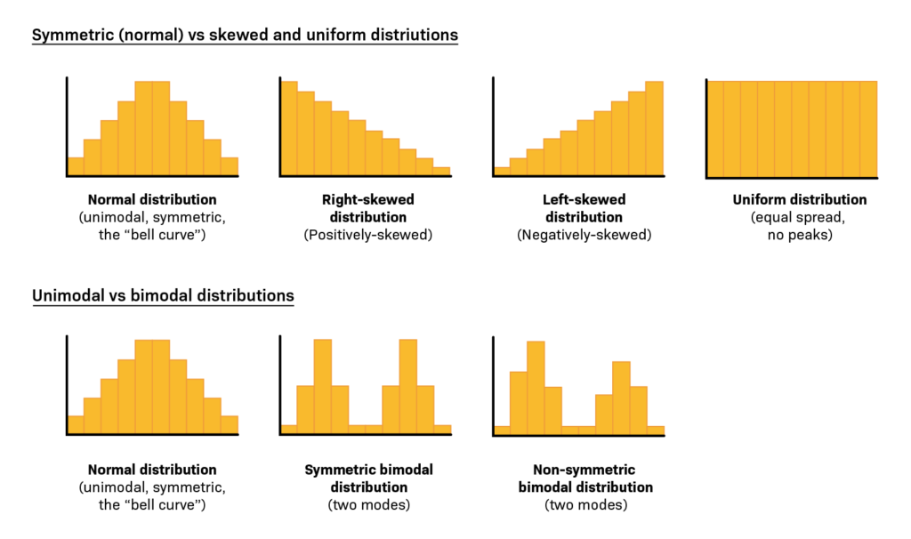
Other Distributions

• Bimodal : It has two distinct peaks, indicating the presence of two separate modes or patterns in the data. This shape suggests that the dataset is a combination of two different underlying distributions.
• Uniform : All values have roughly the same frequency, resulting in a flat, rectangular shape. There are no clear peaks or valleys, and each value has an equal chance of occurrence.
• Multimodal : It has more than two peaks, indicating multiple modes in the dataset. Each peak represents a distinct pattern or subgroup within the data.
• Exponential : It has a rapidly decreasing frequency as values increase. It is characterized by a steep decline in the right tail. The shape is common in datasets where the likelihood of an event decreases exponentially with time.
• Comb: It has alternating high and low frequencies, creating a pattern that resembles the teeth of a comb. This shape suggests periodicity or systematic variation in the data.

5. Normal Q-Q Plot

Furthermore, the Normal Q-Q plot complements the Histogram by providing a visual comparison between the observed data quantiles and the quantiles expected in a normal distribution. By comparing observed quantiles with expected quantiles, researchers gain insights into the conformity of the data to a normal distribution. Clear instructions ensure a seamless incorporation of this method into the normality checking process.

6. Skewness and Kurtosis

It is a statistical measure that quantifies the asymmetry of a probability distribution or a dataset. In the context of data analysis, skewness helps us understand the distribution of values in a dataset and whether it is symmetric or not. The value can be positive, negative, or zero.

• Positive: it indicates that the data distribution is skewed to the right. In other words, the tail on the right side of the distribution is longer or fatter than the left side, and the majority of the data points are concentrated towards the left.
• Negative: Conversely, the data distribution is skewed to the left. The tail on the left side is longer or fatter than the right side, and the majority of data points are concentrated towards the right.
• Zero : A skewness value of zero suggests that the distribution is perfectly symmetrical, with equal tails on both sides.

In summary, skewness provides insights into the shape of the distribution and the relative concentration of data points on either side of the mean.

It is a statistical measure that describes the distribution’s “tailedness” or the sharpness of the peak of a dataset. This helps to identify whether the tails of a distribution contain extreme values. Like skewness, kurtosis can be positive, negative, or zero.

• Positive: The distribution has heavier tails and a sharper peak than the normal distribution. So, It suggests that the dataset has more outliers or extreme values than would be expected in a normal distribution.
• Negative: Conversely,  the distribution has lighter tails and a flatter peak than the normal distribution. Therefore, It implies that the dataset has fewer outliers or extreme values than a normal distribution.
• Zero: A kurtosis value of zero, also known as mesokurtic, indicates a distribution with tails and a peak similar to the normal distribution.

In data analysis,  For a normal distribution, skewness is close to zero, and kurtosis is around 3 (known as mesokurtic). Deviations from these values may suggest non-normality and guide researchers in choosing appropriate statistical methods.

Example of Normality Test

To provide practical insights, this section will present a hypothetical example illustrating the application of normality tests in SPSS. Through a step-by-step walkthrough, readers will gain a tangible understanding of how to apply the Kolmogorov-Smirnov and Shapiro-Wilk tests to a real-world dataset, reinforcing the theoretical concepts discussed earlier.

Imagine you are a researcher conducting a study on the screen time of a group of individuals. You have collected data on the number of min each participant’s screen time per day. As part of your analysis, you want to assess whether the phone screen time follows a normal distribution. Let’s see how to conduct explore analysis in SPSS.

How to Perform Normality Test in SPSS

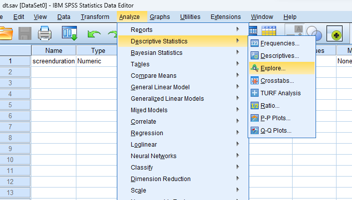
Step by Step: Running Normality Analysis in SPSS Statistics

Practicality is paramount, and this section will guide researchers through the step-by-step process of performing a Normality Test in SPSS. From importing the dataset to interpreting the results, this comprehensive guide ensures seamless execution of the normality testing procedure, fostering confidence in the analytical journey.

• STEP: Load Data into SPSS

Commence by launching SPSS and loading your dataset, which should encompass the variables of interest – a categorical independent variable. If your data is not already in SPSS format, you can import it by navigating to File > Open > Data and selecting your data file.

• STEP: Access the Analyze Menu

In the top menu, locate and click on “ Analyze .” Within the “Analyze” menu, navigate to “ Descriptive Statistics ” and choose ” Explore .” Analyze > Descriptive Statistics > Explore

• STEP: Specify Variables 

Upon selecting “ Explore ” a dialog box will appear. Choose the variable of interest and move it to the “ Dependent List ” box

• STEP: Define Statistics

Click on the ‘Statistics’ button to include Descriptives, Outliers, and Percentiles.

• STEP: Define the Normality Plot with the Test

Click on the ‘Plot’ button to include visual representations, such as histogram, and stem-and-leaf. Check “ Normality plots with tests ” to obtain a Normal Q-Q plot, Kolmogorov-Smirnov Test, and Shapiro-Wilk test .

6. Final STEP: Generate Normality Test and Chart :

Once you have specified your variables and chosen options, click the “ OK ” button to perform the analysis. SPSS will generate a comprehensive output, including the requested frequency table and chart for your dataset.

Conducting the Normality Test in SPSS provides a robust foundation for understanding the key features of your data. Always ensure that you consult the documentation corresponding to your SPSS version, as steps might slightly differ based on the software version in use. This guide is tailored for SPSS version 25 , and any variations, it’s recommended to refer to the software’s documentation for accurate and updated instructions.

SPSS Output for Normality Test

How to Interpret SPSS Output of Normality Test

Interpreting the output of a normality test is a critical skill for researchers. This section will dissect the SPSS output, explaining how to analyze results from the Kolmogorov-Smirnov and Shapiro-Wilk tests, as well as interpret visual aids like Histograms and Normal Q-Q plots.

• Skewness and Kurtosis: The skewness of approximately 0 suggests a symmetrical distribution, while the negative kurtosis of -0.293 indicates lighter tails compared to a normal distribution.
• Kolmogorov-Smirnov Test: The Kolmogorov-Smirnov test yields a statistic of 0.051 with a p-value of 0.200 (approximately), indicating no significant evidence to reject the null hypothesis of normality.
• Shapiro-Wilk Test: The Shapiro-Wilk test produces a statistic of 0.993 with a p-value of 0.876, providing further support for the assumption of normality.
• Histogram and Normal Q-Q Plot: The Histogram with a central peak, reflects a symmetric distribution, and the Normal Q-Q plot with points closely aligned along a straight line, affirming the approximate normality of the “Screen Time (in min)” variable.

How to Report Results of Normality Analysis in APA

Effective communication of research findings is essential, and this section will guide researchers on how to report the results of normality tests following the guidelines of the American Psychological Association (APA). From structuring sentences to incorporating statistical values, this segment ensures that researchers convey their findings accurately and professionally.

Get Help From SPSSanalysis.com

Embark on a seamless research journey with SPSSAnalysis.com , where our dedicated team provides expert data analysis assistance for students, academicians, and individuals. We ensure your research is elevated with precision. Explore our pages;

• SPSS Data Analysis Help – SPSS Helper ,
• Quantitative Analysis Help ,
• Qualitative Analysis Help ,
• SPSS Dissertation Analysis Help ,
• Dissertation Statistics Help ,
• Statistical Analysis Help ,
• Medical Data Analysis Help .

Connect with us at SPSSAnalysis.com to empower your research endeavors and achieve impactful results. Get a Free Quote Today !

Expert SPSS data analysis assistance available.

• [email protected]
• +1 424 666 28 24
• How it works
• GET YOUR FREE QUOTE
• GET A FREE QUOTE
• Frequently Asked Questions
• Become a Statistician

Reporting Normality Test in SPSS

Looking for Normality Test in SPSS ? Doing it yourself is always cheaper, but it can also be a lot  more time-consuming . If you’re not good at SPSS, you can  pay someone to do your SPSS task  for you.

How to Run Normality Test in SPSS: Explanation Step by Step

From the spss menu, choose analyze – descriptives – explore.

A new window will appear. From the left box, transfer variables Age and Height into Dependent list box. Click Both in the Display box.

Click on Statistics… button. A new window will open. Choose Descriptives. Click Continue, and you will return to the previous box.

Click on Plots… button, New window will open. In the Boxplots box, choose Factor levels together. In the Descriptive box, choose Stem-and-leaf and Normality plots with tests. Click Continue, and you will return to the previous box. Click OK.

The test of normality results will appear in the output window.

How to report a Normality Test results: Explanation Step by Step

How to report case processing summary table in spss output.

The first table is the Case Processing summary table. It shows the number and percent of valid, missing and total cases for variables Age and Height.

How to Report Descriptive Statistics Table in SPSS Output?

The second table shows descriptive statistics for variable Age and Height.

How to Report P-Value of Kolmogorov-Smirnov and Shapiro-Wilk tests of normality Table in SPSS Output?

The third table shows the results of Kolmogorov-Smirnov and Shapiro-Wilk tests of normality (tests statistic, degrees of freedom, p-value). Since we have less than 50 observations (N = 32 < 50), we will interpret the Shapiro-Wilk test results.

Firstly, If p (Sig.) > 0.05, we fail to reject the null hypothesis and conclude that data is normally distributed so we must use parametric tests.

secondly, if the p-value is less than 0.05. Therefore, we must reject the null hypothesis in other words data is not normally distributed. Therefore, We must use nonparametric tests.

In our example, the p-value for age is 0.018 < 0.05. Therefore, we must reject the null hypothesis and conclude that age is not normally distributed.

How to Report Normal Q-Q Plot in SPSS output?

The output also shows the Normal Q-Q Plot for Age and Height.

Firstly, If the data points are close to the diagonal line on the chart so we conclude that data is normally distributed otherwise data set does not show normal distribution.

Lastly, From the chart for age, we can conclude that data points are not close to the diagonal line, we, therefore, conclude that data are not normally distributed.

How to Interpret a Normality Test Results in APA Style?

Shapiro-Wilk test of normality was conducted to determine whether Age and Height data is normally distributed. The results indicate that we must reject the null hypothesis for Age data (p = 0.018) and conclude that data is not normally distributed. Consequently, the results also indicate that we fail to reject the null hypothesis for Height data (p = 0.256) and conclude that data is normally distributed.

Visit our “ How to Run Normality Test in SPSS ” page for more details. Moreover, go to the general page to check Other Reporting  Statistical Tests in SPSS . Finally, If you want to watch SPSS videos, Please visit our  YouTube Chanel.

GET HELP FROM THE US

There is a lot of statistical software out there, but SPSS is one of the most popular. If you’re a student who needs   help with SPSS , there are a few different resources you can turn to. The first is  SPSS Video Tutorials . We prepared a page for  SPSS Tutor for Beginners . All contents can guide you through Step-by-step SPSS data analysis tutorials and you can see  How to Run in Statistical Analysis in SPSS .

The second option is that you can get help from us, we give  SPSS help for students  with their assignments, dissertation, or research. Doing it yourself is always cheaper, but it can also be a lot more time-consuming. If you’re not the best at SPSS, then this might not be a good idea. It can take days just to figure out how to do some of the easier things in SPSS. So  paying someone to do your SPSS  will save you a ton of time and make your life a lot easier.

The procedure of the SPSS help service at  OnlineSPSS.com   is fairly simple. There are three easy-to-follow steps.

1.  Click and Get a FREE Quote 2. Make the Payment 3. Get the Solution

Our purpose is to provide quick, reliable, and understandable information about SPSS data analysis to our clients.