short case study on inflation in india

MBA Knowledge Base

Business • Management • Technology

Home » Managerial Economics » Case Study: Inflation in India

Case Study: Inflation in India

Knowing Inflation

By inflation one generally means rise in prices. To be more correct inflation is persistent rise in the general price level rather than a once-for-all rise in it, while deflation is persistent falling price. A situation is described as inflationary when either the prices or the supply of money are rising, but in practice both will rise together. These days economies of all countries whether underdeveloped, developing as well developed suffers from inflation. Inflation or persistent rising prices are major problem today in world. Because of many reasons, first, the rate of inflation these years are much high than experienced earlier periods. Second, Inflation in these years coexists with high rate of unemployment, which is a new phenomenon and made it difficult to control inflation.

An inflationary situation is where there is ‘too much money chasing too few goods’. As products/services are scarce in relation to the money available in the hands of buyers, prices of the products/services rise to adjust for the larger quantum of money chasing them.

Read More: Definition of inflation and it’s types

Inflation is no stranger to the Indian economy. The Indian economy has been registering stupendous growth after the liberalization of Indian economy. In fact, till the early nineties Indians were used to ignore inflation. But, since the mid-nineties controlling inflation has become a priority. The natural fallout of this has been that we, as a nation, have become virtually intolerant to inflation. The opening up of the Indian economy in the early 1990s had increased India’s industrial output and consequently has raised the India Inflation Rate. While inflation was primarily caused by domestic factors (supply usually was unable to meet demand, resulting in the classical definition of inflation of too much money chasing too few goods), today the situation has changed significantly.

Inflation today is caused more by global rather than by domestic factors. Naturally, as the Indian economy undergoes structural changes, the causes of domestic inflation too have undergone tectonic changes. The main cause of rise in the rate of inflation rate in India is the pricing disparity of agricultural products between the producer and consumers in the Indian market. Moreover, the sky-rocketing of prices of food products, manufacturing products, and essential commodities have also catapulted the inflation rate in India. Furthermore, the unstable international crude oil prices have worsened the situation.

Defining causes of Inflation

What exactly is the nature of this inflation which has the nation in its grip? The different causes of inflation which are experienced in Indian economy in a large proportion would be:-

• Demand-pull inflation: This is basically when the aggregate demand in an economy exceeds the aggregate supply. It is also defined as `too much money chasing too few goods’. Bare-boned, it means that a country is capable of producing only 100 items but the demand is for 105 items. It’s a very simple demand-supply issue. The more demand there is, the costlier it becomes. Much the same as the way real estate in the country is rising.
• Cost-push inflation: This is caused when there is a supply shock. This represents the condition where, even though there is no increase in Aggregate Demand, prices may still rise. I.e. non availability of a commodity would lead to increase in prices. This may happen if the costs of especially wage cost rise.
• Imported Inflation: This is inflation due to increases in the prices of imports. Increases in the prices of imported final products directly affect any expenditure-based measure of inflation. They play an important role in driving the rise in domestic prices. The rise in the global prices of crude oil and agricultural commodities, including food grains, and industrial products, and setbacks to global economy resulting from sub-prime mortgage disaster and US recession have contributed to India’s inflation.

Other Causes:

• When the government of a country print money in excess, prices increase to keep up with the increase in currency, leading to inflation.
• Increase in production and labor costs, have a direct impact on the price of the final product, resulting in inflation.
• When countries borrow money, they have to cope with the interest burden. This interest burden results in inflation.
• High taxes on consumer products, can also lead to inflation. An increase in indirect taxes can also lead to increased production costs.
• Inflation can artificially be created through a circular increase in wage earners demands and then the subsequent increase in producer costs which will drive up the prices of their goods and services. This will then translate back into higher prices for the wage earners or consumers. As demands go higher from each side, inflation will continue to rise.
• Debt, war and other issues that cause a drastic financial blunder can also cause the inflation.

Measuring Inflation

Inflation in India is mainly estimated on the basis of fluctuations in the wholesale price index (WPI). The wholesale price index comprises of the following indices:

• Domestic Wholesale Price Index (DWPI)
• Export Price Index (EPI)
• Import Price Index (IPI)
• Overall Wholesale Price Index (OWPI)

The WPI consists of about 435 items and has three broad categories. They are:-

• Primary Articles (weight of 22.0253) — 22% Index
• Fuel, Power, Light, and Lubricants (weight of 14.2262) – 14% Index
• Manufactured Products (weight of 63.7485) — 64% Index

The base year of the WPI is 1993-94. The base year usually chosen is one where there has been fairly less volatility. The Indian WPI figure is released weekly on every Thursday. But recently the government has approved the proposal to release a wholesale price based inflation data on a monthly basis, instead of every week. The new series of WPI based inflation with 2004-05 as the base year would be launched soon. The move is aimed at improving the accuracy of the inflation data.

The monthly release of WPI is a widely-followed international practice. And, it is expected to improve the quality of data. Collection of price data of manufactured products will, accordingly, have a monthly frequency consistent with the practice of release of WPI. The new series of WPI based inflation with 2004-05 as the base year would be launched soon. However, the government will continue to release a weekly index for primary articles, and commodities in the fuel, power, light and lubricants groups. The weekly index will facilitate monitoring of prices of agricultural commodities and petroleum products, which are sensitive in nature.

Problems of Inflation

It has been reported that the manufacturing capacity in India is running around 95 per cent, which usually means it is running at full capacity. Therefore, when the price of manufactured products is increasing, it means that demand is usually higher than supply and that is a clear case of demand-pull inflation.

On the primary goods front, which consists of fruits, vegetables, food-grains etc, it is not that straight-forward. It has certainly been all over the news that the prices of fruits and vegetables are increasing and a trip to the supermarket or local grocery shop will testify to that. Although it is a clear case of demand-pull inflation, on the other, it is also a bit of a supply shock when one considers the fact that there is an abnormally high percentage of fruits and vegetables that goes to waste because of the lack of cold-storage facilities. Some estimates say 50 per cent of produce goes to waste and that is a conservative number.

The fuel price hike is a straight example of cost push inflation. When OPEC (The Organization of the Petroleum Exporting Countries) was formed, it squeezed the supply of oil and this caused oil prices to rise, contributing to higher inflation. Since oil is used in every industry, a sharp rise in the price of oil leads to an increase in the prices of all commodities.

The in depth problems due to inflation would be:

• When the balance between supply and demand goes out of control, consumers could change their buying habits, forcing manufacturers to cut down production.
• Inflation can create major problems in the economy. Price increase can worsen the poverty affecting low income household.
• Inflation creates economic uncertainty and is a dampener to the investment climate slowing growth and finally it reduce savings and thereby consumption.
• The producers would not be able to control the cost of raw material and labor and hence the price of the final product. This could result in less profit or in some extreme case no profit, forcing them out of business.
• Manufacturers would not have an incentive to invest in new equipment and new technology.
• Uncertainty would force people to withdraw money from the bank and convert it into product with long lasting value like gold, artifacts.

The imbalances inflation has created in the Indian economy:-

• It has created a new rich class in social and political lives who are corrupt themselves and also corrupt the overall society.
• The increased prices reduced the capacity to save and people preferred present consumption to future consumption.
• It has provided protection and subsides to industries which bred inefficiency.
• It has lead to misallocation of resources due to distortion of relative prices and finally a redistribution of wealth from the poor to the rich.
• It disturbs balance of payments.

Curbing Inflation

There are several reasons why we should worry about the spike in the inflation rate. Inflation is a tax on the poor and long-term lenders. Inflation is already too high, though it is definitely not at economy-wrecking levels. But it’s best to be serious about the threat it poses. Inflation has emerged as the biggest risk to the global outlook, having risen to very high levels across the world, levels that have not been generally seen for a couple of decades.

Currently, in India, we go through boom-and-bust cycles; sometimes GDP growth rates are very high and sometimes GDP growth rates drop sharply. This boom-and-bust cycle is unpleasant for every household. There is a powerful international consensus that stabilizing inflation reduces this boom-and-bust cycle of GDP growth.

India is facing the problem of inflationary pressure because of the increase in Aggregate Demand while Aggregate Supply is respectively constant. The inflationary pressure faced by Indian Economy is due to Demand-Pull inflation i.e. Aggregate Demand > Aggregate Supply. Thus to curb inflation need to fill the gap between Aggregate Demand and Aggregate Supply. For this either we need to increase Aggregate Supply or decrease Aggregate Demand that can hamper economic development. To increase Aggregate Supply either there is a need to increase production capacity of all current production units or to build new production plants.

But as quoted in a survey done by RBI that all the production plants are running at their full production capacity thus all resources are full employed. The other way is to build new plant but to do this will take at least 18months to 2years. Thus meanwhile we need to decrease Money Supply, which is opted by RBI. Increasing production of useful goods and services is what India should focus on.

As in the short run it is not possible to meet the gap between Aggregate Demand and Aggregate Supply thus RBI is planning to decrease liquidity by reducing Money Supply from the market. RBI planned that Liquidity from the market can be drained by decreasing money supply and to do so it is increasing CRR, repo rate, reverse repo rate and taking other measure like that.

CRR i.e. Cash Reserve Ratio (Liquidity Ratio) is the percentage of deposit that a commercial bank needs to keep with RBI by which RBI control liquidity in the market and create Money Supply. Repo Rate is the rate at which RBI lends money to other commercial Banks.

The Reserve Bank said that such decisions had been taken to curb inflation in India. RBI is taking positive steps to reduce the inflation since inflations rates are going up week by week. By raising the reserve rate, a deflationary pressure can be put on the economy, since the money multiplier has been reduced. People will therefore save more. But in this hike, there is negative impact in terms of higher interest rates and personal loans, vehicle loans and other loans become costly. RBI may hike the rate to reduce the money circulation in the country but it also decreased the sales of all loan items and further it reduces the manufacturing activity of many industries. Now the public and private sector banks may raise the interest rate at which they lend money to borrowers.

Produce more exports than imports than another country, then your money deflates with respect to that currency. Exporting becomes a problem cause buyers from outside feel that the goods are expensive so they prefer buying some other country’s goods with cheaper rate. Thus money does not come in. in the same way, when public has more money they buy foreign goods, thus money goes out which is bad. There is a need to encourage people to purchase goods produced within the country.

It is important for policymakers to make credible announcements and degrade interest rates. Private agents must believe that these announcements will reflect actual future policy. If an announcement about low-level inflation targets is made but not believed by private agents, wage-setting will anticipate high-level inflation and so wages will be higher and inflation will rise. A high wage will increase a consumer’s demand (demand pull inflation) and a firm’s costs (cost push inflation), so inflation rises. Hence, if a policymaker’s announcements regarding monetary policy are not credible, policy will not have the desired effect.

Keynesians emphasize reducing demand in general, often through fiscal policy, using increased taxation or reduced government spending to reduce demand as well as by using monetary policy. Supply-side economists advocate fighting inflation by fixing the exchange rate between the currency and some reference currency such as gold. This would be a return to the gold standard. All of these policies are achieved in practice through a process of open market operations.

As individuals what can we do to stop Inflation?

Firstly save!!! As much of your money as possible should be saved. This will reduce the demand on the economy and hopefully reduce inflation. Do not overuse daily essentials like cooking gas, electricity etc. Cut down on inessentials when buying groceries. Look for cheaper alternatives to products that you normally buy.

Keep roads, highways, sidewalks, etc., beautified to help attract tourism and bring additional monetary into a growing economy. Stop illegal immigration. Illegal activities reap the benefits of the country but don’t pay taxes. Government-backed investment schemes such as Post Office Savings Schemes, Public Provident Funds (PPF) and National Savings Certificates (NSC) are best to invest in when inflation is slowly inching up and you are only looking at safety, not returns. Invest in short term deposits and funds, commodities and property. This will help you to slowly reach your financial goals while safeguarding your hard-earned money.

Read More: Treasury bills and inflation control

Related posts:

• Definition of Inflation – Types of Inflation
• Case Study: Advertising Strategies of The Times of India
• Case Study: McDonald’s Business Strategies in India
• Case Study: L’Oreal Marketing Strategies in India
• Case Study: Coffee Cafe Business in India
• Case Study on MNC’s Marketing Strategies: In India, it’s a Brand New Way
• Case Study of Kishore Biyani: India’s Retail King
• Case Study of Maggi: Brand Extension and Repositioning in India
• Case Study on Vodafone’s Re-Branding Strategies in India: Hutch to Vodafone
• The Stages of Inflation

Leave a Reply Cancel reply

Your email address will not be published. Required fields are marked *

• Open access
• Published: 21 June 2022

The impact of macroeconomic factors on food price inflation: an evidence from India

• Asharani Samal   ORCID: orcid.org/0000-0001-8275-0267 1 ,
• Mallesh Ummalla 2 &
• Phanindra Goyari 1  

Future Business Journal volume  8 , Article number:  15 ( 2022 ) Cite this article

5 Citations

Metrics details

The present study investigates the impact of macroeconomic factors on food price inflation in India utilizing the monthly time series during January 2006–March 2019. The long-run relationship is confirmed among the variables using the ARDL bounds testing approach to cointegration. The coefficients of long-run estimates show that per capita income, money supply, global food prices, and agricultural wages are positively and significantly impacted food price inflation in both the short and long-run. While food grain availability has a negative and significant impact on food price inflation in both the short-run and long run. Further, the short-run estimates revealed that real exchange rate positively impacts food price inflation. However, the coefficient is insignificant in the short-run. The Granger causality estimates show that a short-run bidirectional causality is confirmed among per capita income, the exchange rate, per capita net availability of food grain and food price inflation. Further, there is evidence of unidirectional causality running from global food prices to food price inflation. However, there is no causal relationship running from money supply and agricultural wages to food price inflation in the short-run.

Introduction

The main objective of monetary policy in any economy is to maintain price stability. However, high food price inflation affects not only macroeconomic stability but also small farmers and poor consumers of the developing country where poor people spend their massive portion of income on food consumption. Agricultural commodity price volatility negatively impacts all societies by causing macroeconomic instability; specifically, it affects the impoverished that spend a large portion of their resources on food and fuel [ 47 ]. Therefore, high food price inflation has become a significant concern among the researchers and policymakers in determining responsible factors to surge in food price inflation. The high food price inflation has been experienced in the recent period due to increasing demand for biofuels in many developed countries, increasing demand for various diets among newly prosperous populations as compared to the production of such foodstuff, rise in minimum support prices, rapid regional economic growth, increasing the cost of fertilizers and other inputs, rising oil prices, etc.

Agriculture is very competitive in producing homogenous goods, given its vulnerability and high dependence on monsoon. It also contributes 17% of gross domestic product and employs more than 50% of the population. However, the contribution of the agricultural sector to GDP has been declining substantially since 2014, and the growth of agriculture is likely to increase by 2.1% in 2018–19 [ 23 ]. Further, price of agricultural products is more volatile than the non-agricultural sector due to high dependence on climate change. Therefore, attention should be given to the agricultural sector and the behavior of agriculture prices, especially for developing countries like India, where the majority of the population depends on agriculture. The persistent and high food price inflation over the period has gained more extensive attention in India by the researchers and policymakers as food price inflation has been the major contributor behind the increase in overall Wholesale Price Index (WPI) inflation in India [ 2 ]. Further, agricultural price is susceptible to relative changes in input prices, supply factors, etc.

Theoretically, rising food prices are basically due to two factors in the literature, i.e., real and monetary shocks. These are explained by structuralist and monetarist approaches, respectively. According to structuralists, the money supply is passive, and the real shocks in a particular sector tend to upsurge in food price inflation. Hence, inflation occurs in the prices of other goods. However, monetarists argued that inflation could arise through an autonomous increase in money supply via generating aggregate demand, which increases the relative price of commodities. Therefore, an increase in money supply is a cause for inflation, not necessarily by real shocks.

However, the developing countries like India are not exceptional from higher food prices and macro-economic instability. Since the 1991 economic reforms, the Indian economy has maintained a single-digit economic growth rate and moderate inflation. However, in recent years, one of the major problems that the Indian economy is facing is higher food price inflation. The WPI food price inflation was documented 10.20% during January 2008–July 2010 [ 33 ]. Further, CPI-IW for food was experienced at 8.05% during 2006–2019 while it was recorded at 13%, especially in 2013. However, the growth rate of gross food grain production was 2.66% during this period. The demand for food commodities increases at a higher rate due to the high economic growth rate (7–9%) per annum. In contrast, the annual growth of agriculture is relatively low (1.5%) compared to the service sector and GDP growth [ 40 ]. The total investment in agriculture has been reduced from 2.43 to 1.28% during 1979–80 to 2007–08 period [ 28 ]. The expenditure on subsidies, maintenance of existing projects, the relatively lower allocation for irrigation, rural infrastructure and research, lack of adequate credit support, and credit infrastructure in rural areas are the drivers of slow growth in public investment in agriculture [ 43 ]. Given this high food price inflation, researchers and policymakers have raised severe concern about reducing the food price inflation because most of the population spend half of the income on food expenditure, and food containing a larger share in the CPI basket. Therefore, it is necessary to find the causes and suitable majors to reduce food price inflation.

The present study contributes to food price inflation literature in several ways. First, a wide range of studies has investigated the drivers of food price inflation in India. The various demand and supply-side factors, namely, per capita income, growth of money supply, changing patterns of the consumer's dietary habits, high agricultural wages, speculations, and low growth of agricultural productions, are accountable for high food inflation. However, the results are ambiguous and vary considerably across countries due to different data periods and econometric methodologies applied in their studies. Second, the change in macroeconomic factors may have a substantial effect on food price inflation. For instance, if the food prices positively impact money supply, the consumer suffers from welfare loss. If it negatively effects on food prices, the producer suffers from welfare loss. However, this relationship of macroeconomic factors has not empirically analyzed significantly with respect to food price inflation in India. Third, various studies have explored the impact of macroeconomic factors on food price inflation across the world. For example, Kargbo [ 24 ] for Eastern and Southern Africa, Kargbo [ 25 ] for West Africa, Reziti [ 38 ] for Greek, Kargbo [ 26 ] for South Africa, Yu [ 46 ] for China and Sasmal [ 40 ]. Nevertheless, few studies have empirically examined the impact of selected macroeconomic factors on food price inflation by incorporating a control variable like per capita net availability of food grain into account. To the best of my knowledge, there is no study existing in the context of India. Fourth, most of the studies have taken WPI food indices, food items from only primary food articles or some of the index of selected food items, such as cereals and pulses, fruits and vegetables, milk and milk products, egg, meat, and fish as a measure of food price inflation. However, the present study has used the combined price index for industrial worker food (CPI-IW-F). Fifth, numerous studies have concluded that food price inflation is triggered by supply-side factors (see, [ 11 , 17 , 33 ]). However, to examine the rise in food price inflation, we have included both demand and supply-side factors in our study. Six, the present study also considered that food price inflation is not only influenced by domestic factors but also by global factors. More specifically, changes in global food prices and the exchange rate might positively and significantly impact food price inflation. However, the effect of these external factors on food price inflation does not explain the extent of food price inflation driven by domestic supply-side factors. For this purpose, we have included the per capita net availability of food grain as a control variable in the model. Suppose the demand for agricultural food items rises remarkably owing to a surge in macroeconomic factors. However, the supply of food items failed to meet the demand proportionately, then food items prices will go up. Therefore, the goal of the present study is to analyze the long-run and short-run impact of macroeconomic factors on food price inflation and verify the causal relationship aspect of these variables in the case of India over the period January 2006–March 2019.

The remaining of the paper is structured as follows. “ Literature review ” section follows the review of the literature on the relationship between macroeconomic factors and food price inflation. “ Methods ” section represents data and methodology. “ Results and discussion ” section discusses the results of the study. “ Conclusions ” section provides conclusive remarks and policy implications.

Literature review

This paper aims to examine the impact of macroeconomic factors on food price inflation. This section provides a review of the literature to establish the empirical basis of the link between macroeconomic factors and food price inflation.

Per capita income and food price inflation

Per capita income has a positive impact on food price inflation via increasing purchasing power of the money in the hands of the people, which leads to a surge in demand for food items resulting in a rise in food prices. Carrasco and Mukhopadhyay [ 10 ] argued that per capita income is positively affected food prices in three South Asian economies. However, the decline in agricultural production increases food prices up, and magnitudes are varying across countries. Agrawal and Kumarasamy [ 1 ] documented that food price inflation rose with the response to increases in India’s per capita income. They also suggested a 1% surge in per capita income upsurges the demand for fruits, vegetables, milk, and edible oil by 0.55–0.65%, and animal products by 0.38%. However, it reduces the demand for cereals and pulses by 0.05% and 0.20%, respectively. Joiya and Shahzad [ 22 ] and Sasmal [ 40 ] reported the same findings in Pakistan and India, respectively. In contrast, the study also found a negative association between food price inflation and per capita income. Kargbo [ 24 ] in Ethiopia and Malawi among Eastern and Southern African countries, Kargbo [ 25 ] for Cote d'Ivoire of West African countries.

Money supply and food price inflation

An increase in the money supply positively affects food price inflation through market credit facility by generating aggregate demand. However, it reduces food prices by creating investment via availing credit to the producer. Numerous studies have investigated the impact of money supply on food price inflation across the world. For example, Mellor and Dar [ 29 ] found that the expansion of money supply largely determines upward pressure on food grains prices. Barnett et al. [ 5 ] found that money supply positively affects food inflation and agricultural commodity prices in the U.S. Similar results were found by Kargbo [ 26 ] and Asfaha and Jooste [ 3 ] for South Africa. Further, Bhattacharya and Jain [ 8 ] concluded that an unexpected monetary tightening induces food price inflation in emerging and developed countries. However, a negative relationship is established between money supply and food prices for Kargbo [ 24 ], Kargbo [ 25 ], and Yu [ 46 ] for Eastern and Southern African countries and West African countries and China.

Exchange rate and food price inflation

The depreciation of the real exchange rate increases food price inflation by expanding the cost of importing petroleum products, fertilizer, and other finished products relating to agricultural commodities, leading to rising domestic market prices. In other words, depreciation of the exchange rate directly affects the agricultural sectors vi changing the prices of tradable and non-tradable goods resulting in a change in the prices of agricultural products in favor of the farmer. Taylor and Spriggs [ 45 ] showed that the exchange rate has a greater influence on volatility of agricultural prices in Canada. Similarly, Mitchell [ 30 ] and Mushtaq et al. [ 32 ] and Iddrisua and Alagidede [ 19 ] also concluded that the depreciation of the exchange rate is positively affected food prices in the U.S., Pakistan and South Africa, respectively. In contrast to this, Cho et al. [ 12 ] confirmed that change in the exchange rate has a negative impact on relative agricultural prices. However, Sasmal [ 40 ] found no significant relationship between the exchange rate and food price inflation in India during 1971–2012.

Global food price and food price inflation

The increase in the global food price of the commodity can influence the domestic price via international trade mechanism. The export increases as the global food price increases resulting in a decrease in domestic market supply followed by a hike in prices. On the contrary, the rise in import raises the domestic substitute food item’s price followed by a surge in domestic market price. Robles [ 39 ] indicated that the international prices transmission has a positive impact on the domestic agricultural market in Asian and Latin American countries. Gulati and Saini [ 16 ] revealed that the global food price index is positively impacted food price inflation in India. Similarly, Baltzer [ 4 ] states that an increase in international prices promotes domestic prices in the case of Brazil and South Africa. However, the price.

transmission is very limited in China and India. Lee and Park [ 27 ] confirmed that the lagged values of global food price inflation are positively impacted food price inflation in 72 countries. Selliah et al. [ 41 ] revealed that an increase in global food price increases domestic food prices in both the short and long run in Sri Lanka. Similarly, Holtemöller and Mallick [ 17 ], Bhattacharya and Sen Gupta [ 6 ], and Huria and Pathania [ 18 ] also documented that global food price shocks have a significant and positive inflationary trend on food inflation in India. However, Rajmal and Mishra [ 37 ] pointed out a limited transmission of prices from international food prices to domestic prices in India.

Agricultural wage and food price inflation

One of the significant public work programs is the National Rural Employment Guarantee (NREG), which promotes the real daily agricultural wage rates. On the one hand, an increase in rural wages can induce food prices by increasing production costs. On the other hand, it raises food prices via higher purchasing power, resulting in higher wages, which boosts the demand for food items. Gulati and Saini [ 16 ] revealed that domestic farm wages are positively associated with food price inflation in India. Goyal and Baikar [ 15 ] showed that the rapid increase in MGNREGA wages when it merged with inflation boosts agricultural wages rather than the implementation of MGNREGA across India. Bhattacharya and Sen Gupta [ 6 , 7 ] examined the drivers of food price inflation in India over the period 2006–2013. The structural vector error correction model (SVECM) showed that agricultural wage inflation promotes food price inflation after the implementation of MNGREGS.

The above literature review shows that both demand and supply-side factors have contributed to food price inflation. Many studies have investigated the impact of macroeconomic factors on food price inflation across the globe. However, only a few studies have been directed, which empirically examined the effect of macroeconomic factors on food price inflation by incorporating per capita net availability of food grain and agricultural wages in a multivariate framework. So far as we know, there is no study available in the case of India in this regard employing monthly data over the period January 2006–March 2019. Hence, our study attempts to fill this gap.

The present study makes use of monthly time series data on per capita GDP (Y), real exchange rate (EX), money supply (M3), global food price index (GF), per capita net availability of food grain (NFG), agricultural wages (AW) and combined price index-industrial workers for food (CPI-IW-F) indices as a proxy for food price index (FP) during January 2006–March 2019. The data on per capita GDP, real exchange rate, money supply is collected from the Reserve Bank of India (RBI), whereas combined price index-industrial workers for food and agricultural wages are retrieved from the Ministry of Labor Bureau, Government of India. The data on per capita net availability of food grain and real global food price index are obtained from the Directorate of Economics and Statistics, Department of Agriculture & Farmers Welfare, Government of India, and the Food and Agriculture Organization of the United Nations, respectively. Monthly data on per capita net availability of food grain and per capita GDP is not available in the case of India. Therefore, we have used the linear interpolation method to get the monthly data for this variable. Footnote 1 The selection of the data period has been considered based on the availability of uniform and consistent monthly data over a period of time. We use high-frequency data while working on macroeconomic variables to capture the true impact of it [ 31 ]. Further, data on food price inflation is volatile, measuring the impact of macroeconomic factors on food inflation using high-frequency data, namely, weekly and monthly, provides accurate estimates rather than annual series. Since, data on a targeted variable i.e., food inflation is not available on a weekly basis for a longer period in the case of India. Therefore, we have used monthly data for this purpose.

The real exchange rate (EX) is measured as the real effective exchange rate which is trade based weighted average value of Indian currency against 36-currency bilateral weights, per capita income (Y) is measured as the percentage change in per capita gross domestic product, money supply (MS) is measured as broad money (MS), global food prices (GF) are measured as a real global food price index, and agricultural wages (AW) is measured as average daily wage rates from agricultural occupations; per capita net availability of food grain (NFG) is measured as gross production plus net imports plus stocks. Finally, food price inflation (FP) is measured as combined price index-industrial workers for food index (CPI-IW-F). The food inflation was experienced in India from 2006 onwards. However, the CPI-combined series is used and available from 2014 onwards to measure the official inflation rate. To get a more extended frequency of data on food inflation series, we have used consumer price index-industrial workers for food (CPI-IW-F) as a proxy for food inflation measures. We select to use CPI-IW-F because Bicchal and Durai [ 9 ] and Goyal [ 14 ] established that CPI-IW and CPI-combined have similar properties with CPI-IW is available for a more extended period. All the variables are seasonally adjusted using CENSUS X13 and converted into the natural logarithm form except per capita GDP.

Unit root tests

One should necessarily check the properties of all the variables before commencing any econometric techniques as it gives spurious and invalid results. The ARDL technique requires to check the integration properties of the selected variables to confirm that none of the variables should follow I (2) process, which seems to be invalid and unsuitable for applying the ARDL approach. Therefore, we use the ADF and PP tests to check the order of integration of the variables.

ARDL bounds testing approach to cointegration

We employ the ARDL bounds testing approach to cointegration propounded by Pesaran and Shin [ 35 ] and Pesaran et al. [ 36 ] in order to examine the long-run and short-run association between macroeconomic factors and food price inflation in India. This method is superior over other traditional approaches of Johansen and Juselius [ 21 ] and Johansen [ 20 ] cointegration on the following grounds. First, it is one of the most popular and flexible methods. It does not impose any restriction on any nature of data and can be applied irrespective of all the order of integration I (1) or I (0) or both mix. Second, as noted by Pesaran and Shin [ 35 ] that ARDL estimators give the true parameters, and coefficients are super consistent as compared to other long-run estimates, especially when the sample size is small. Third, it also helps to eradicate the problem of the endogeneity that appears in the model. Fourth, it is even able to capture both short-run and long-run estimates simultaneously. The unrestricted error correction models (UECM) of the ARDL model can be represented as follows:

where ∆ denotes first difference operator; \({\varepsilon}_{t}\) is the error term; \({\alpha }_{1}\) , \({\alpha }_{2}\) , \({\alpha }_{3}\) , \({\alpha }_{4}\) , \({\alpha }_{5}\) , \({\alpha }_{6}\) , and \({\alpha }_{7}\) are the constant; \({\alpha }_{F}\) , \({\alpha }_{Y}\) , \({\alpha }_{M}\) , \({\alpha }_{E}\) , \({\alpha }_{G}\) , \({\alpha }_{NF}\) , and \({\alpha }_{A}\) are the long-run coefficients; \({\beta }_{h}\) , \({\beta }_{i}\) , \({\beta }_{j}\) , \({\beta }_{k},{\beta }_{l}, {\beta }_{m}\) and \({\beta }_{n}\) are the short-run coefficients.

The optimal lag selection has been made based on the Akaike Information Criteria (AIC). The primary step in the ARDL model is to estimate the Eqs. ( 1 – 7 ) by ordinary least squares (OLS). The long-run relationship is determined based on the F test or Wald test for the coefficient of the lagged levels of the variables. The null hypothesis of no long-run relationship, \({H}_{0}:{\alpha }_{F}={\alpha }_{Y}={\alpha }_{M}={\alpha }_{E}={\alpha }_{G}={\alpha }_{NF}={\alpha }_{A}=0\) against the alternative hypothesis of the long-run, \({H}_{1}:{\alpha }_{F}\ne {\alpha }_{Y}\ne {\alpha }_{M}\ne {\alpha }_{E}\ne {\alpha }_{G}\ne {\alpha }_{NF}\ne {\alpha }_{A}=0\) referred to the equation follows as (FP/Y, MS, EX, GF, NFG, AW). According to Pesaran et al. [ 37 ], the null hypothesis of no long-run association can be rejected if F -statistics is greater than the upper critical bound (UCB). It suggests that there is a long-run association among the variables. While, test statistics falls below the lower critical bound (LCB), null hypothesis cannot be rejected. It suggests that there is no long-run association among the variables. If the calculated value falls between the lower and upper critical points, the result is inconclusive. Because the two asymptotic critical values bound lower value (assuming the regressors are I (0)) and upper (assuming purely I (1) regressors) provide a test for cointegration.

After identifying the long-run relationship among the variables, our next step is to apply the vector error correction model to examine the directions of causality among the variables in both the short-run and long-run. The model of VECM can be written as follows.

where \(\Delta\) is the difference operator; \({ECM}_{t-1}\) is the lagged error correction term, which is derived from the long-run cointegration relationship; \({\varepsilon}_{1t}\) , \({\varepsilon}_{2t}\) , \({\varepsilon}_{3t}, {{\varepsilon}_{4t}, \varepsilon}_{5t}, {\varepsilon}_{6t}\) and \({\varepsilon}_{7t}\) are the random errors; \({\gamma }_{1}\) , \({\gamma }_{2}\) , \({\gamma }_{3, }{\gamma }_{4, }{\gamma }_{5, }{ \gamma }_{6}\) and \({\gamma }_{7}\) are the speed of adjustments. The long-run relationship among the variables indicates that there is a presence of Granger-causality at least one direction, which is determined by F -statistics and lagged error correction term. The short-run causal relationship is represented by F- statistics on the explanatory variables while long-run causal relationship is represented by t-statistics on the coefficient of the lagged error correction term. The error correction term ( \({ECT}_{t-1}\) ) is negative and statistically significant (t-statistic) at the 1% significance level.

Results and discussion

Preliminary analysis.

A preliminary analysis is conducted using commonly used descriptive statistics. We also reported the summary of descriptive statistics of all the considered variables during the study period in Table 1 . The results revealed that the average food price index and the real exchange rate is 5.375% and 4.687% during the study period. However, the average money supply and real global food price index is 11.185% and 4.619%. The per capita net availability of food grain and agricultural wages is 5.130% and 6.931% whereas, per capita income is 0.445%, which is lower than other variables across the sample period. The results of the correlation matrix are represented in Table 2 . The correlation analysis results revealed that per capita income, money supply, real exchange rate, real global food price index, per capita net availability of food grain and agricultural wages are positively associated with food price inflation. For instance, food price inflation is highly correlated with per capita income, money supply, real exchange rate, per capita net availability of food grain, and agricultural wages. It suggests that macroeconomic factors might be promoting food price inflation in India. Similarly, per capita income is positively correlated with money supply, exchange rate, and per capita net availability of food grain, and agricultural wages. Further, there is a high positive correlation between agricultural wages and per capita net availability of food grain.

Results of unit root tests

To avoid spurious and invalid results of all the non-stationary data, we have checked the integration properties of all the variables and confirm that none of the variables follows the I (2) process. Therefore, the ADF and PP unit root tests are used to check the order of integrations of the variables. The results of unit root tests are reported in Table 3 . It indicates that food price inflation (FP), per capita income (Y), money supply (MS), real exchange rate (EX), real global food price index (GF), per capita net availability of food grain (FG) and agricultural wages (AW) are integrated of order I (1).

Results of ARDL cointegration tests

The above unit root test results show that all variables follow a same order of integration, i.e., I (1). Therefore, we apply the ARDL technique to check the long-run relationship among the variables using Eqs. ( 1 )-( 7 ) during January 2006–March 2019. Here, the optimal lag length is 2, according to VAR lag order selection criteria. The results of the ARDL model are presented in Table 4 . The result shows that calculated F -statistics (4.155) is larger than UCB at the 5% level of significance when food price inflation is considered a dependent variable (FP/Y, MS, EX, GF, NFG, WA). It indicates that there is a long-run relationship among food price inflation (FP) and per capita income (Y), money supply (MS), real exchange rate (EX)), global food prices (GF), per capita net availability of food grain (NFG), and agricultural wages (WA). Likewise, calculated F- statistics (11.043) is also larger than UCB at the 5% level of significance when per capita income is considered a dependent variable and integrated order (1). Therefore, UCB is applied to establish a long-run relationship among the variables. Likewise, calculated F- statistics (10.239) is also larger than UCB at the 5% level of significance when money supply (MS) is considered a dependent variable. Similarly, calculated F- statistics (3.335) is also larger than UCB at the 10% level of significance when global food price (GF) is considered a dependent variable. However, calculated F -statistics is lower than UCB when the exchange rate (EX), per capita net availability of food grain (NFG), and agricultural wages (AW) serve as dependent variables. It suggests a there is no long-run relationship among the variables when the exchange rate, per capita net availability of food grain and agricultural wages are the dependent variables.

Results of long-run and short-run estimates

The cointegration test results based on the ARDL model revealed the long-run equilibrium relationship among the variables. However, these results do not explain the cause-and-effect association among the food price inflation and macroeconomic factors, namely, per capita income, money supply, exchange rate, global food prices, per capita net availability of food grains, and agricultural wages. Hence, we have investigated the impact of macroeconomic factors on food price inflation in this part. It is better to check the long-run effect of macroeconomic factors on food price inflation after confirming the cointegration relationship among the variables when food price inflation is considered the dependent variable. The results of the long-run analysis are reported in Table 5 in panel-I. The long-run results illustrate that per capita income is positively and significantly impacted food price inflation. It implies that a one unit increase in per capita income induces food price inflation by 0.14 unit. The rise in per capita income raises the purchasing power of the money, which leads to a surge in demand for food items resulting in a hike in food prices. The results of our study similar to Carrasco and Mukhopadhyay [ 10 ] in three South Asian economies, Agrawal and Kumarasamy [ 1 ] in India, Joiya and Shahzad [ 22 ] in Pakistan and Sasmal [ 40 ] in India. However, our result is inconsistent with Kargbo [ 24 ] and Kargbo [ 25 ], who revealed a negative relation between the variables in Ethiopia and Malawi, and in Cote d'Ivoire, respectively.

Similarly, a 1% increase in money supply increases food price inflation by 0.36%. It implies that the rise in money supply puts upward pressure on food price inflation and is significant at the 1% level of significance. Money supply is positively affecting food price inflation by generating aggregate demand in the market, which pushes the food prices up. This finding is consistent with Kargbo [ 24 ] for Kenya, Sudan, and Tanzania among the Eastern and Southern African countries and contradictory with Sasmal [ 40 ] who did not find any long-run relationship between money supply and food price inflation in India and Yu [ 46 ] for China who confirmed that monetary policy expansion has a negative impact on prices of seven major food products in the long-run. Similarly, a rise in the real exchange rate has a downward pressure on food price inflation. It indicates that a 1% increase in the real exchange rate will have a negative impact on food price inflation by 0.30%. The increase in the real exchange rate reduces food prices by lowering the import of petroleum products, fertilizer, and other products relating to agricultural commodities in the long run. Hence, organic fertilizers can be used to produce commercial food products to reduce the dependency on fertilizers, which may maintain price stability and reduce the negative welfare impact on food prices. This outcome is consistent with Cho et al. [ 12 ] and is inconsistent with Iddrisua and Alagidede [ 19 ] in South Africa, Durevall et al. [ 13 ] in Ethiopia. Further, per capita net availability of food grain has a negative impact on food price inflation. In other words, there is an inverse relationship between per capita net availability of food grains and food price inflation in India. It suggests that a 1% increase in per capita net availability of food grains reduces food price inflation by 0.69%. The increase in the supply of net food availability in the domestic market by increasing food production can reduce food price inflation. On the other hand, if the supply of food grain availability declines due to crop failure, it increases food price inflation. Therefore, the government should increase domestic food production and reduce the exports of commodities at the time of food inflation to maintain stability in prices. Further, agricultural production is seasonal, and it is highly correlated to the month of food harvest. The stock of food grain during harvest season can avoid the off seasonal food price inflation. Increasing the stock of food items by establishing a larger cold storage system and strengthen and widening the existing warehouses can also help to control food inflation in India. This result is similar to Kargbo [ 25 ] in Cote d’Ivoire and Nigeria and Carrasco and Mukhopadhyay [ 10 ] in three South Asian economies and inconsistent with Sasmal [ 40 ], who failed to establish a significant relationship between agricultural food production and food price inflation in India in the long-run. Furthermore, our results revealed that food price inflation rose with the response to increases in global food prices. It suggests that a 1% surge in global food price upsurges food price inflation by 0.13%. This result is consistent with Selliah et al. [ 41 ] for Sri Lanka, Holtemöller and Mallick [ 17 ] for India, and Huria and Pathania [ 18 ] for India. However, Rajmal and Mishra [ 37 ] and Baltzer [ 4 ] pointed out a limited transmission of prices from international food prices to domestic prices in India. The extent of transmission of global food prices on price hike in the domestic market depends on at which magnitudes commodity’s international trade takes place. Finally, our study results also found that agricultural wages have a positive and significant impact on food price inflation at the 1% level of significance. It implies that a 1% surge in agricultural wages increases the food price inflation by 0.31% in the long-run. The rise in wage rate via welfare-oriented-schemes like MNGREGS increases the bargaining and purchasing power of money, increasing in demand for food items followed by increased food inflation. The increase in the agricultural wage rate should be substituted with food price inflation by increasing productivity. Hence, the increase in demand for food originated by a hike in the agricultural wage rate can be substituted by raising the productivity of each worker. A similar result is found by Bhattacharya and Sen Gupta [ 7 ] for India.

After having discussed long-run results, we shall move in to discuss with reference to the short-run. The results of the short-run analysis are reported in Table 5 in panel-II. The short-run analysis indicates an increase in per capita income and money supply is positively related to food price inflation in the short-run as the coefficients of these variables are statistically significant. Similarly, food price inflation rises with the increase in global food prices. Further, the real exchange rate has a positive impact on food price inflation in the short-run. However, the result is not significant. Moreover, agricultural wages have a positive impact on food price inflation. It implies that an increase in agricultural wages raises food price inflation in the short run. The outcome is consistent with Huria and Pathania [ 18 ] for India. However, per capita net availability of food grain is negatively and significantly impacted food price inflation. It suggests that a 1% increase in food grain availability decreases food price inflation by 0.11% in the short-run. In contrast, a decrease in the growth rate of food grain availability increases food price inflation. This finding is similar to Kargbo [ 25 ] in Cote d’Ivoire and Senegal among West African countries. Finally, the results also documented lagged food price inflation positively impacts present food price inflation. It suggests that a 1% increase in lagged food price upsurges food price inflation by 0.36% in the short run.

The sign of lagged ECT is negative and significant at the 1% level, which implies that short-run deviation from food prices can be restored toward the long-run equilibrium with a 16.8% speed. The model has satisfied all the diagnostic tests. This model is free from autoregressive conditional heteroscedasticity; the functional form of the model is well specified, which is represented by the Ramsey RESET coefficient.

Results of VECM Granger causality test

After identifying the long-run association between macroeconomic factors and food price inflation, we have employed the VECM Granger causality test to examine the directions of causality among the variables in both the short-run and long-run. The Granger causality results are represented in Table 6 . The outcomes of the short-run causality tests are obtained from the F -statistics of lagged independent variables, while the results of long-run causality are obtained from the negative and significant coefficients of t-statistics of lagged error correction term. The results are reported in Table 6 and show that a short-run bidirectional causality is confirmed between per capita income, exchange rate, and food price inflation at a 1% level. This finding is opposite of Sasmal [ 40 ], who reported a unidirectional causality running from per capita income to food price inflation in India. Similarly, a bidirectional causality is existed between percapita net availability of food grain and food price inflation in the short run. It implies that the increase in food grain availability reduces food price inflation by increasing domestic food grain production on the one hand. Whereas on the other hand, an increase in food price inflation also leads to a rise in food grain availability by rising demand for food products. Further, there is a unidirectional causality running from global food prices to food price inflation. It suggests that an increase in global price attracts exporters to increase their supply of food items to the global market to get high profit, which eventually decreases the domestic market supply, resulting an in a price increase. However, there is no causal relationship running from money supply and agricultural wages to food price inflation in the short run.

There is an existence of a bidirectional causal relationship between global food prices and per capita income. However, no causality runs from money supply, exchange rate, per capita net availability of food grain, and agricultural wages to per capita income. A short run unidirectional causality is established from food price inflation, exchange rate, global food prices, and per capita net availability of food grain to money supply. A bidirectional causality has existed between agricultural wages and money supply in the short run. Further, unidirectional causality is running from per capita income, the exchange rate to global food prices. A unidirectional causal relationship is found from per capita income, money supply, the exchange rate, and global food prices to per capita net availability of food grain in the short run. Moreover, short-run unidirectional causality is confirmed from food price inflation, per capita income, the exchange rate and global food prices to agricultural wages.

Moving to the long-run causality, the coefficients of \({ECM}_{t-1}\) are negative and statistically significant in Eq. ( 8 ), where money supply, global food prices, and per capita net availability of food grain are the dependent variables. Therefore, results revealed a bidirectional causality among the money supply, global food prices, and per capita net availability of food grain production in the long-run.

Conclusions

This study aimed to examine the impact of macroeconomic factors on food price inflation in India during January 2006–March 2019. To consider the short-run dynamics and the long-run analysis and directions of causality among the variables, we have applied the ARDL model and Granger causality test in our study. The ARDL results have shown evidence of the long-run association among the macroeconomic factors and food price inflation. The long-run result show that percapita income, money supply, global food price, and agricultural wages have a positive and significant impact on food price inflation of India in both the long-run and short run. However, the per capita net availability of food grain negatively impacts food price inflation. It implies that an increase in food grain availability reduces food price inflation in both the short and long run. Further, the real exchange rate is positively affecting food price inflation. However, it is insignificant in the short-run. The Granger causality estimates show that a short-run bidirectional causality is confirmed among per capita income, the exchange rate, per capita net availability of food grain, and food price inflation. Further, there is evidence of unidirectional causality running from global food prices to food price inflation. However, there is no causal relationship running from money supply and agricultural wages to food price inflation in the short run. The long-run results revealed a bidirectional causality among the money supply, global food prices and per capita net availability of food grain.

Given these results, the paper makes important contribution to the macroeconomic factors and food price inflation in India. The significant policy suggestions are that the growth in money supply promotes food price inflation in the long-run, which affects the welfare of the poor consumer as the majority of the people depend on agriculture. It also positively affects market credit facility by generating aggregate demand followed by changes in relative prices across commodities, which push the food prices up. Therefore, the government should adopt effective policy measures to protect consumers from higher food prices. These are the effectively implementation of public distribution systems, policies for food security, and reducing the money supply via adopting a contractionary monetary policy, which eventually reduces food price inflation by reducing demand for food items. Further, the increase in global food inflation triggers food price inflation by international trade channels. However, the influence of global food inflation on food price inflation can be moderated by introducing a flexible tariff structure. Hence, the government should introduce stable and liberal trade policies that reduce food price inflation without compromising farmers remuneration values.

Moreover, our result also revealed that an increase in the net availability of food grain reduces food price inflation in both the short and long run. Therefore, the government should take necessary steps in favor of an increase in domestic food production. The high yielding variety (HYV) seeds, easily accessible credit facilities should be available to the farmer, increasing the domestic agricultural food production, thereby reducing the import of agricultural goods through the exchange rate and their adverse impact on food inflation. The stock of food grain during harvest season can avoid off seasonal food inflation. The increasing the stock of food items by establishing an extensive cold storage system and strengthening large warehouses can control food inflation in India. Furthermore, the rise in agricultural wages boosts food price inflation. The increase in the agricultural wage rate should be substituted with food price inflation by increasing labor productivity. Hence, the increase in demand originated by a hike in the agricultural wage rate can be substituted by raising each workers productivity.

Our results also found that per capita income Granger causes food price inflation both in the short-run. In this respect, we can say that there is a huge sectoral imbalance among the sectors. The government should be more focused on the agricultural sector and its growth and productivity by allocating massive funds in the irrigation, agricultural research, and innovation of modern technology and its adaptation in agriculture instead of spending on the name of social security and welfare of the poor. Therefore, balanced and sustainable growth and stability can be achieved for a developing country like India. The real exchange rate and food price inflation Granger causes to each other. The depreciation of the real exchange rate increases the food price inflation via expanding the import of petroleum products, fertilizer, and other finished products relating to agricultural commodities, which are very expensive. The increasing import of these products promotes food price inflation by raising domestic prices. Hence, to reduce the food price inflation, the government should increase the domestic agricultural production to meet our demand for food items rather than importing from other countries.

Availability of data and materials

Data used in the study are available in the Reserve Bank of India, Ministry of Labor Bureau, Directorate of Economics and Statistics, Department of Agriculture & Farmers Welfare, Government of India, and the Food and Agriculture Organization of the United Nations.

By using the linear interpolation method, we have converted the annual data into the monthly time series data. Because the high-frequency data increases the power of a statistical test and provide robust results [ 48 ]. The interpolation method has been widely used in the empirical analysis [ 34 , 42 , 44 ].

Abbreviations

Autoregressive distributed lag

Combined price index

Wholesale price index

Reserve Bank of India

Agrawal P, Kumarasamy D (2014) Food price inflation in India: causes and cures. Indian Econ Rev 49(1):57–84

Google Scholar  

Anand R, Ding D, Tulin V (2014) Food inflation in India: the role of monetary policy. IMF working paper-14/178

Asfaha TA, Jooste A (2007) The effect of monetary changes on relative agricultural prices. Agrekon 46(4):460–474

Article   Google Scholar  

Baltzer K (2013) International to domestic price transmission in fourteen developing countries during the 2007–08. [In] Food crisis food price policy in an era of market instability. Oxford University Press, Oxford

Barnett RC, Bessler DA, Thompson RL (1983) The money supply and nominal agricultural prices. Am J Agric Econ 65(2):303–307

Bhattacharya R, Sen Gupta A (2017) What role did rising demand play in driving food prices up? South Asian J Macroecon Public Finance 6(1):59–81

Bhattacharya R, Sen Gupta A (2018) Drivers and impact of food inflation in India. Macroecon Finance Emerg Mark Econ 11(2):146–168

Bhattacharya R, Jain R (2020) Can monetary policy stabilise food inflation? Evidence from advanced and emerging economies. Econ Model 89:122–141

Bicchal M, Durai SRS (2019) Rationality of inflation expectations: an interpretation of Google Trends data. Macroecon Finance Emerg Mark Econ 12(3):229–239

Carrasco B, Mukhopadhyay H (2012) Food price escalation in South Asia. Econ Polit Wkly 47(46):59–70

Chand R (2010) Understanding the nature and causes of food inflation. Econ Polit Wkly 9XLV(9):10–13

Cho G, Kim M, Koo WW (2005) Macro effects on agricultural prices in different time horizons. Meeting of the American Agricultural Economics Association, Providence, Rhode Island

Durevall D, Loening J, Birru Y (2013) Inflation dynamics and food prices in Ethiopia. J Dev Econ 104:89–106

Goyal A (2015) Understanding high inflation trend in India. South Asian J Macroecon Public Finance 4(1):1–42

Goyal A, Baikar AK (2015) Psychology, cyclicality or social programmes: Rural wage and inflation dynamics in India. Econ Pol Wkly 50:116–125

Gulati A, Saini S (2013) Taming food inflation in India. Commission for Agricultural Cost and Prices, Discussion paper 4. Ministry of Agriculture, Government of India

Holtemöller O, Mallick S (2016) Global food prices and monetary policy in an emerging market economy: the case of India. J Asian Econ 46:56–70

Huria S, Pathania K (2018) Dynamics of food inflation: assessing the role of intermediaries. Glob Bus Rev 19(5):1363–1378

Iddrisu AA, Alagidede IA (2020) Monetary policy and food inflation in South Africa: A quantile regression analysis. Food Policy 91: 101816.

Johansen S (1991) Estimation and hypothesis testing of cointegration vectors in Gaussian vector autoregressive models. Econometrica 59(6):1551–1580

Johansen S, Juselius K (1990) Maximum likelihood estimation and inference on cointegration with applications to the demand for money. Oxf Bull Econ Stat 52(2):169–210

Joiya S, Shahzad A (2013) Determinants of high food prices: the case of Pakistan. Pak Econ Soc Rev 51(1):93–107

Kapoor A (2018) Competitiveness in agriculture will boost other sectors, Business standard, June 05, retrieved from https://www.business-standard.com/article/news-ians/competitiveness-in-agriculture-will-boost-other-sectors-column-active-voice-118060500301_1.html

Kargbo JM (2000) Impacts of monetary and macroeconomic factors on food prices in eastern and Southern Africa. Appl Econ 32(11):1373–1389

Kargbo JM (2005) Impacts of monetary and macroeconomic factors on food prices in West Africa. Agrekon 44(2):205–224

Kargbo JM (2007) The effects of macroeconomic factors on South African agriculture. Appl Econ 39(17):2211–2230

Lee HH, Park C Y (2013) International transmission of food prices and volatilities: a panel analysis. Asian Development Bank economics working paper series (373). https://doi.org/10.2139/ssrn.2323056

Mani H, Bhalachandran G, Pandit VN (2011) Public investment in agriculture and GDP growth: Another look at the intersectoral linkages and policy implications. Working paper no. 201, Centre for Development Economics, Delhi School of Economics

Mellor JW, Dar AK (1968) Determinants and development implications of food grains prices in India, 1949–1964. Am J Agric Econ 50(4):962–974

Mitchell D (2008) A note on rising food prices. World Bank policy research working paper series no. 4682

Modugno M (2013) Now-casting inflation using high frequency data. Int J Forecast 29(4):664–675

Mushtaq K, Awan DA, Abedullah A, Ahmad F (2011) Impact of monetary and macroeconomic factors on wheat prices in Pakistan: implications for food security. Lahore J Econ 16(1):95–110

Nair S, Eapen L (2012) Food price inflation in India (2008 to 2010). Econ Polit Wkly 47(20):46–54

Paramati SR, Bhattacharya M, Ozturk I, Zakari A (2018) Determinants of energy demand in African frontier market economies: an empirical investigation. Energy 148:123–133

Pesaran MH, Shin Y (1999) An autoregressive distributed lag modelling approach to cointegration analysis. In: Strom S (ed) Econometrics and economic theory in 20th century: the Ragnar Frisch centennial symposium, Chapter 11. Cambridge University Press, Cambridge

Pesaran MH, Shin Y, Smith RJ (2001) Bounds testing approaches to the analysis of level relationships. J Appl Economet 16(3):289–326

Rajmal, Mishra S (2009) Transmission of international food prices to domestic food prices The Indian evidence. RBI staff studies, Department of Economic Analysis and Policy, S S (DEAP):6/2009

Reziti I (2005) The relationship between macroeconomic variables and relative price variability in Greek Agriculture. Int Adv Econ Res 11(1):111–119

Robles M (2011) Price transmission from international agricultural commodity markets to domestic food prices: case studies in Asia and Latin America. IFPRI, Washington, DC

Sasmal J (2015) Food price inflation in India: the growing economy with sluggish agriculture. J Econ Finance Admin Sci 20(38):30–40

Selliah S, Applanaidu SD, Hassan S (2015) Transmission of global food prices to domestic prices: evidence from Sri Lanka. Asian Soc Sci 11(12)

Shahbaz M, Arouri M, Teulon F (2014) Short- and long-run relationships between natural gas consumption and economic growth: evidence from Pakistan. Econ Model 41:219–226

Sivagnanam KJ, Murugan K (2016) Impact of public investment on agriculture sector in India. J Econ Soc Dev 12(2):45–51

Tang CF, Chua SY (2012) The savings-growth nexus for the Malaysian economy: a view through rolling sub-samples. Appl Econ 44(32):4173–4185

Taylor J, Spriggs J (1989) Effects of the monetary macro-economy on Canadian agricultural prices. Can J Econ 22(2):278–289

Yu X (2014) Monetary easing policy and long-run food prices: evidence from China. Econ Model 40:175–183

Zhang Z, Lohr L, Escalante C, Wetzstein M (2010) Food versus fuel: What do prices tell us? Energy Policy 38(1):445–451

Zhou S (2001) The power of cointegration tests versus data frequency and time spans. South Econ J 67(4):906–921

Download references

Acknowledgements

Not applicable.

The authors declare that no funding from any agencies was received for this study.

Author information

Authors and affiliations.

School of Economics, University of Hyderabad, Hyderabad, 500046, India

Asharani Samal & Phanindra Goyari

School of Business, Woxsen University, Hyderabad, 502345, India

Mallesh Ummalla

You can also search for this author in PubMed   Google Scholar

Contributions

AS: Conceptualization, methodology, software, formal analysis, data curation, writing—original draft, reviewing and editing. MU: Resources, data curation, writing—reviewing and editing. PG: Resources, supervision and editing. All authors have read and approved the final manuscript.

Corresponding author

Correspondence to Asharani Samal .

Ethics declarations

Ethics approval and consent to participate, consent for publication, competing interests.

The authors declare that they have no competing interests.

Additional information

Publisher's note.

Springer Nature remains neutral with regard to jurisdictional claims in published maps and institutional affiliations.

Rights and permissions

Open Access This article is licensed under a Creative Commons Attribution 4.0 International License, which permits use, sharing, adaptation, distribution and reproduction in any medium or format, as long as you give appropriate credit to the original author(s) and the source, provide a link to the Creative Commons licence, and indicate if changes were made. The images or other third party material in this article are included in the article's Creative Commons licence, unless indicated otherwise in a credit line to the material. If material is not included in the article's Creative Commons licence and your intended use is not permitted by statutory regulation or exceeds the permitted use, you will need to obtain permission directly from the copyright holder. To view a copy of this licence, visit http://creativecommons.org/licenses/by/4.0/ .

Reprints and permissions

About this article

Cite this article.

Samal, A., Ummalla, M. & Goyari, P. The impact of macroeconomic factors on food price inflation: an evidence from India. Futur Bus J 8 , 15 (2022). https://doi.org/10.1186/s43093-022-00127-7

Download citation

Received : 02 July 2021

Accepted : 15 May 2022

Published : 21 June 2022

DOI : https://doi.org/10.1186/s43093-022-00127-7

Share this article

Anyone you share the following link with will be able to read this content:

Sorry, a shareable link is not currently available for this article.

Provided by the Springer Nature SharedIt content-sharing initiative

• Food price inflation
• Macroeconomic factors
• ARDL bounds testing approach
• Causality test

JEL Classification

• Business News
• India Business News
• Explained in charts: India's inflation situation and its impact on households

Explained in charts: India's inflation situation and its impact on households

Visual Stories

PPF Calculator

This financial tool allows one to resolve their queries related to Public Provident Fund account.

FD Calculator

When investing in a fixed deposit, the amount you deposit earns interest as per the prevailing...

NPS Calculator

The National Pension System or NPS is a measure to introduce a degree of financial stability...

Mutual Fund Calculator

Mutual Funds are one of the most incredible investment strategies that offer better returns...

Other Times Group News Sites

Popular categories, hot on the web, trending topics, living and entertainment, latest news.

The dynamics of survey-based household inflation expectations in India

IIM Ranchi Journal of Management Studies

ISSN : 2754-0138

Article publication date: 13 December 2021

Issue publication date: 1 March 2022

The author analyzes households' inflation expectations data for India, collected quarterly by the RBI for more than a decade. The contribution of this paper lies in two folds. First, this study examines the relationship between relatively recent inflation expectations survey of households (IESH) and the actual inflation for India. Secondly, the author employs a structural VAR with the time period 2006 Q2 to 2020 Q2 on inflation expectation survey data of India. A short-term non-recursive restriction is imposed in the model in order to capture the simultaneous co-dependence causal effect of inflation expectation and realized inflation.

Design/methodology/approach

This paper studies the dynamic behavior of inflation expectations survey data in two folds. First, the author analyzes the time series property of the survey data. The author begins with testing the stationarity property of the series, followed by the casual relationship between the expected and actual inflation. The author further examines the short-run and long-run behavior of the IESH with actual inflation. Employing autoregressive distributed lag and Johansen co-integration, the author tested if a long-run relationship exists between the variables. In the second approach, the author investigates the determinants of inflation expectations by employing a non-recursive SVAR model.

The preliminary explanatory test reveals that inflation expectation is a policy variable and should be used in monetary policy as an instrument variable. The model identifies the price puzzle for India. The author finds that the response of inflation to a monetary policy shock is neutral. The results also indicate that the expectations of the general public are self-fulfilling.

Originality/value

IESH has only commenced from September 2005, hence is relatively new as compared to other survey in developed countries. Being a new data set so far, the author could not locate any study devoted in analyzing the behavior of the data with other macroeconomic variables.

• Inflation expectations
• Monetary policy

Impulse response function

Jha, S. (2022), "The dynamics of survey-based household inflation expectations in India", IIM Ranchi Journal of Management Studies , Vol. 1 No. 1, pp. 38-54. https://doi.org/10.1108/IRJMS-08-2021-0109

Emerald Publishing Limited

Copyright © 2021, Saakshi Jha

Published in IIM Ranchi Journal of Management Studies . Published by Emerald Publishing Limited. This article is published under the Creative Commons Attribution (CC BY 4.0) licence. Anyone may reproduce, distribute, translate and create derivative works of this article (for both commercial and non-commercial purposes), subject to full attribution to the original publication and authors. The full terms of this licence may be seen at http://creativecommons.org/licences/by/4.0/legalcode

1. Introduction

Every central bank faces the challenge of keeping the inflation rate within reasonable limits. One of the main factors that determine the rate of inflation is the inflation expectations of various macroeconomic agents in an economy. Thus, central banks try to keep the inflation expectations “well-anchored” primarily by making their policy for targeting inflation public and by sharing the data on the inflation expectations of professional forecasters and the general public. While these policies have been an inherent part of the central banks in developed countries, it is only recently that India has begun following a similar path.

Inflation expectations can influence the behavior of economic agents. The inter-temporal decisions like savings, investments, wage negotiations, etc., made by economic agents are highly dependent on their expectations about future inflation. These inter-temporal decisions, in turn, affect economic activity, which further influences actual inflation. If the current inflation rate creates expectations for future inflation, which itself is induced by the expectations of the economic agents, it leads to the creation of an “inflation expectations spiral” in the economy. The effect of the “inflation expectations spiral” can cause high and persistent inflation, thereby reducing the effectiveness of monetary policy for controlling inflation.

In order to control inflation and to avoid the trap of “inflation expectations spiral,” the monetary policymakers must know the pattern and behavior of expected inflation. Berk (2002) indicates that any effect of monetary policy on inflation expectations depends upon the direction and intensity of the causality between the inflation expectations and actual inflation. Ball et al. (2005) point out that the dynamic correlation between inflation expectations and realized inflation will help anchor inflation expectations and strengthen the credibility of central banks. In other words, a strong co-relationship between the realized and expected inflation will allow monetary policy to achieve price stability for the economy.

Several studies have presented different conclusions on the relationship between inflation expectations and actual inflation. Among those finding inflation expectations to be self-fulfilling, Leduc et al. (2007) prove inflation expectations to be the cause of the high and persistent US inflation rate of the 1970s. Mavroeidis et al. (2014) study shows that inflation expectations could cause inflation in a self-fulfilling spiral. Other studies, on the other hand, conclude that actual inflation has significant effects on inflation expectations. The expectations-augmented Phillips Curve predicts that actual and expected inflation would move in a coordinated and balanced relationship ( Phelps, 1967 ). Furthermore, studies like Chen (2008) demonstrate a significant positive correlation between the expectations of future inflation and current actual inflation. Feng and Zhu (2012) study document a causal relationship from expected inflation to actual inflation.

In addition to the unidirectional nexus indicated by the above literature, other studies support a bi-directional relationship between inflation expectations and actual inflation. Patra and Ray (2010) certify bidirectional causality between the inflation expectations and the actual inflation. They state that the increase in inflation may cause an increase in inflation expectations, which will further drive up inflation. Reid (2015) finds a causal relationship between realized inflation and inflation expectations in South Africa. The change in inflation occurs first, followed by a similarly adjusted change in expectations. Using impulse responses, Kim and Lee (2013) illustrate the dynamic effects on actual inflation due to the shocks of the inflation expectation for Asian countries.

Previous research provides evidence of opposing and supporting the lead-lag relationship between expected and actual inflation and even supporting the bi-directional linkages. The existence of such vivid literature indicates the importance of the studies. Our study, highly intertwined with the existing literature, attempts to identify the relationship between actual and expected inflation for India.

The contribution of this paper to the existing literature is as follows. First, this study examines the relationship between relatively recent inflation expectations survey of households (IESH) and the actual inflation for India. The survey has only commenced from September 2005; hence it is relatively new than other surveys in developed countries. Being a new data set so far, we could not locate any study devoted to analyzing the behavior of the data with other macroeconomic variables. Second, like other developed countries, India recently (June 2016) has formally adopted inflation targeting as its framework. With inflation targeting as its framework, analyzing the dynamic behavior of inflation expectations becomes of paramount importance.

This paper studies the dynamic behavior of inflation expectations survey data in two folds. First, we analyze the time series property of the survey data. We begin with testing the stationarity property of the series, followed by the casual relationship between the expected and actual inflation. Our study reveals inflation expectations survey data to be stationary at the first difference and indicates a causal relationship between actual consumer price index (CPI) and wholesale price index (WPI) inflation and the expected inflation. Second, we proceed further by examining the short-run and long-run behavior of the IESH with actual inflation. Employing autoregressive distributed lag (ARDL) and Johansen co-integration, we test if a long-run relationship exists between actual CPI and WPI inflation and households' inflation expectations survey data.

Further, use structural vector auto regressive (SVAR) model to study the various determinants of inflation expectation and their effects on economic variables and inflation. We construct a four-variable VAR with the output gap, nominal interest rate, inflation and inflation expectation as our endogenous variable. We impose a non-recursive restriction in our VAR, as inflation expectation attributes simultaneous co-dependence causal effect with realized inflation.

Inflation in India is measured by the WPI and CPI. WPI measures the inflation from the producer side as its basket constitutes wholesale goods. The CPI is mainly considered as consumer side inflation as the basket consists of consumer goods. In our analysis for both the dynamic nature of inflation expectations and the SVAR, we use CPI as our realized inflation. Since inflation expectations collected by RBI are household survey data, we believe that a lot of general public expectations must be based on the price of their day-to-day consumption. Hence CPI comes into play. Secondly, we find a long-run correlation of survey data with CPI and not WPI inflation. Moreover, the lagged CPI inflation shows a better correlation with survey data than the lagged WPI.

This paper is organized in the following manner: Section 2 explains the data set used for the analyses. Next, Section 3 reports on the unit root test results for analyzing the stationarity of the data and the Granger causality results. Further, Section 4 explains the long-run relationship between realized inflation and the IESH. Section 5 provides the genesis of structural vector autoregressive (SVAR), Section 6 presents the results, and Section 7 concludes.

2.1 Inflation expectations survey of households [1]

Reserve Bank of India (RBI) initiated a survey of the inflation expectations of the general public (IESH) since September 2005. The survey has both qualitative and quantitative responses regarding the changes in price levels and the rate of inflation for three months and one year ahead.

The survey data has been published in the public domain since September 2006. Recently, the 63rd round of the survey concluded, collecting responses from around 6,000 households. A visual representation of survey-based inflation expectations variable and actual inflation gives us a quick idea about how these series move over time.

Figure 1 reveals the relationship between household inflation expectations and actual inflation: CPI and WPI. In the initial period, Figure 1 depicts a lag relationship of inflation expectations with the CPI inflation. It could be said; initially, the inflation CPI is leading the public perception in a very early stage of the survey. This pattern of households' inflation expectations and actual CPI inflation can only be witnessed till the 2008 financial crisis. During the global recession of 2007–08, the public expectations about inflation were higher than the actual CPI inflation.

Similarly, the highest peak in actual inflation was witnessed in the second quarter of 2009 (15.2%), whereas the expectations were at their highest four-quarters earlier, i.e. in the second quarter of 2008 (13.5%). Since that time, the expectations have always responded to the CPI with lags. The trend that is clear from the figure is that the expectations, no matter the situation in the economy, have always remained higher than the actual CPI inflation.

Unlike the CPI inflation, the earlier observations show that expectations are in line with the WPI inflation. Until the second quarter of 2008, the general public's expectations followed the WPI inflation, i.e. during the same period the highest peak was obtained for all of the variables. The divergence in the data is seen after this, i.e. when the WPI inflation drops, the expectations fall in response, but then they rise again. One reason for this rise in inflation expectations may be CPI inflation. The CPI inflation increased to 15.3% in quarter two of 2009. Hence, this may have pulled the inflation expectations up. Looking at the data, we believe that since WPI has been the policy variable in India for a long time, people's expectations in the starting quarters were based on it. Gradually, as the survey proceeded, the public began relating their expectations to the prices of the basket of goods consumed by them rather than WPI. Hence, we find that expectations started to connect more to CPI rather than WPI, despite the latter being the policy variable until 2016.

Table 1 contains the statistical summaries of the variables of our interest. Both CPI and WPI are positively and significantly correlated with the three-month-ahead inflation expectations. A quick observation of the results shows inflation CPI (mean – 7.49 and std. dev. – 2.89) to be closely associated with the three-months ahead mean households' inflation expectations (mean – 9.60 and std. dev. – 2.31) than the WPI inflation (mean – 4.58 and std. dev. – 3.71).

2.2 Output gap

To generate the output gap, we collect the Gross Domestic Product (GDP) at factor cost from the RBI database on the Indian economy. The output gap is the difference between the seasonally adjusted real GDP series using the X-11 ARIMA method and the trend computed through the HP filter.

All the other data like CPI inflation, WPI inflation and repo rate is obtained from the database of the Indian economy (DBIE), RBI. The analysis runs from the second quarter of 2006 until the second quarter of 2020. The survey data on inflation expectations is available in the public domain from the second quarter of 2006 onward; hence, we commence our analysis from this period.

3. Empirical analysis

This part of our study is an attempt to better understand the survey-based inflation expectations of the general public. We begin by exploring the economic relation of inflation expectations with actual or realized inflation by investigating the time-series properties of the former. We start by testing the stationarity property for both CPI and WPI of inflation, with a particular focus on the tests meant for small samples; then we analyze the causality relation between the two series on realized and survey-based inflation expectations, and, finally, examine the existence of a long-run relationship between the series.

3.1 Stationarity property

As a first step in determining the time-series properties of survey-based inflation expectations, we investigate its stationarity property. A stationary time series has a constant mean and variance over time. We check the hypothesis that IESH has no systematic trend, no systematic change in the variance and no periodicity or seasonality to the series.

We investigate the presence of a unit root with the following four tests – augmented Dickey–Fuller (ADF), Phillips Perron (PP), Dickey–Fuller generalized least square (DF-GLS), and Ng-Perron. The reason for using all four tests is as follows. The ADF and PP tests are widely used in the unit root literature, though they suffer from drawbacks. The ADF test is known to have low power, and the PP test does not perform well with small samples ( Davidson and Mackinnon, 2004 ).

Perron and Ng (1996) , Elliot et al. (1996) and Ng and Perron (2001) have modified the traditional ADF and PP tests to mitigate the size distortion and to increase the power of each test for every persistent alternative. We incorporate these tests for our time series data since the sample size is small and provides the robustness check.

Elliot et al. (1996) proposed an efficient test modifying the Dickey–Fuller test statistic using a generalized least square (GLS) method. They demonstrate that the modified test has the best overall performance in small sample size and power tests, conclusively dominating the standard Dickey–Fuller test. In particular, Elliott et al. (1996) find that their “DF-GLS” test “has substantially improved power when an unknown mean or trend is present.”( 1996 , p. 813).

Therefore, the DF-GLS and NG-Perron [2] unit root tests are also conducted, as they perform better with small samples. All these tests deliver robust results, suggesting that the series is stationary.

Table 2 indicates that all the variables are stationary at first difference.

3.2 Pairwise Granger causality

As outlined in the Introduction section, inflation expectations are an essential variable for policymakers since this variable might both affect and get affected by actual or realized inflation. Therefore, a two-way causal relationship is suspected between these two variables. We investigate whether such a relationship prevails between survey-based inflation expectations and actual CPI and WPI inflations in India. The results of the Granger causality tests are presented in Table 3 .

Results from Table 3 support the hypothesis that a causal relationship exists between the CPI inflation and inflation expectations. CPI inflation comprises the prices of consumer goods and services; a two-way relationship between CPI inflation and inflation expectations of the general public is justified. For WPI inflation, we find a mixed result. Table 3 first row indicates a weak acceptance of the null hypothesis of inflation expectations with WPI inflation. At the same time, the vice-versa does hold. One of the reasons for such a discrepancy could be that the general public relates more to the prices of the goods they regularly consume rather than the wholesale prices relevant to the producers. This was perhaps the primary reason why the Urjit Patel Committee Report in 2014 recommended that CPI inflation be the official measure of inflation instead of the WPI inflation. It was formally accepted as an official measure of inflation in 2016 by RBI.

On identifying the causal relationship between the actual and expected inflation, we try to identify the short- and long-run relationship between them. The two econometric approaches widely used to determine the short and long-run relationship are the ARDL – ECM and vector error correcting method (VECM) approach.

Both approaches mentioned above have their specifications like ARDL – ECM can only be used when anyone series is stationary at I(0). In contrast, VECM is used when series are integrated at I(1) and are co-integrated in the long run. In our case, all our series are stationary at I(1) (as depicted in Table 2 ). However, in the literature, there is debate regarding the stationarity of the inflation series. Juselius (2006) mentions that inflation series can be stationary at a level if the series is considered for more extended periods; otherwise, the series remains non-stationary. Since the time period of survey-based inflation data is limited in the Indian context, it is not surprising that the data series is stationary at the first difference and not at levels. However, Reid (2015) estimates the ARDL –ECM (error correction model) and VECM model for measuring the stickiness of survey-based inflation expectations for South Africa for 40 observations. The study considers inflation to be stationary at both levels and the first difference. Following the same line, we also analyze the long-run relationship of households' survey-based inflation expectations with actual inflation using the ARDL and VECM approach.

3.3 ARDL bound testing approach

Considering that the actual inflation can also be stationary at the level, we examine the long-run relationship between inflation expectations and realized inflation following the ARDL bound test approach to co-integration developed by Pesaran et al. (2001) . ARDL is considered a better way of testing a long-run relationship. Firstly, it can be used for series that are not stationary at the same level, i.e. it can be applied to the series irrespective of I(0) or I(1). Secondly, it can simultaneously estimate short-run and long-run parameters. Thirdly, it has better small sample properties ( Smyth and Narayan, 2006 ). The following unrestricted error correction model is estimated for ARDL: (1) Δ IESH t =   α 01 +   α 12 IESH t − 1 +   α 21 InfCPI t − 1 +   ∑ i = 0 p α 1 i Δ IESH t − i + ∑ j = 0 q α 1 j   Δ InfCPI t − j +   ε t (2) Δ IESH t =   α 02 +   α 12 IESH t − 1 +   α 22 InfWPI t − 1 + ∑ i = 0 p α 1 i   Δ IESH t − i + ∑ j = 0 q α 1 j   Δ InfWPI t − j + μ t Where, Δ is the first difference operator, α 01 is the constant, α 12 and α 21 are the long-run coefficients and α i and α j represents the short-run coefficients. The ε t is the white noise error term. The optimal lag structure for the ARDL approach is determined by Schwarz Bayesian information criterion. We estimate equation 2 to determine the long-run relation of IESH with inflation WPI.

To determine the long-run relationship between the variables, two separate bound tests are performed: a Wald or F -test for the joint null hypothesis H 0 : α 12  =  α 21  = 0 and a t -test on lagged dependent variable. The asymptotic distribution of the F -test is non-standard; one can use the value of the critical bound provided by Pesaran et al. (2001) . There are two asymptotic critical values computed by Pesaran et al. (2001) ; one at I(0), that variables are considered not to be co-integrated, and second at I(1) when variables are co-integrated. The I(0) is regarded as lower critical bound (LCB) and I(1) as upper critical bound (UCB). If the test statistic exceeds the UCB, then the variables are co-integrated in the long run. Additionally, if the test statistic is below the LCB, the null hypothesis of no co-integration is not rejected. On the other hand, if test statistics lie between LCB and UCB, the results are inconclusive. equation (1) and equation (2) in the ARDL version of the error correction model can be expressed as equation (3) and (4) , respectively below. (3) Δ IESH t =   α 01 + ∑ i = 0 p α 1 i   Δ IESH t − i + ∑ j = 0 q α 1 j   Δ InfCPI t − j   +   λ ECM t − 1 +   ϵ t (4) Δ IESH t =   α 02 + ∑ i = 0 p α 1 i   Δ IESH t − i + ∑ j = 0 q α 1 j   Δ InfWPI t − j   +   λ ECM t − 1 + ε t Where, λ is the speed of adjustment parameter, and ECM is the residuals obtained from the estimated co-integration model of equations (1) and (2) . The α 1 i and α 1 j if significant, provides evidence on the direction of the short-run causation while a significant t -statistic for the ECM depicts the presence of significant long-run causation.

Table 4 presents the bound test result. The calculated F -statistics (5.53) is greater than the UCB at a 10% significance level for CPI inflation. Whereas for WPI inflation, the F -statistics is lower than UCB for all the significance levels. Hence we conclude based on the results that there exists no co-integration relation between IESH and WPI inflation. This inspection of IESH with CPI and WPI inflation separately provides us with some insight, but because the results obtained are not significant at a higher degree as well as the unit root result proves the actual inflation series to be stationary at I(1), we avoid the ARDL regression. In order to establish the long-run relationship, we run a VECM. The result of which is present in the next section.

4. Long-run co-integration between inflation expectations and realized inflation

The causality test above indicates the actual CPI and WPI inflation cause households’ inflation expectation. The linear relationship between the two variables can be expressed as equation 5 . (5) π t e =   α + β π t + e t Where, π t e is the inflation expectations and π t is the actual inflation. The econometric analysis of equation 5 is possible only when the relationship as established is stable. For a stable relationship, the variables should be stationary. Our unit root test suggests that the households' inflation expectations and actual inflation are non-stationary at levels, thereby stationary at I(1). Being non-stationary, there is a high tendency that these variables may not converge to equilibrium in the long run.

Moreover, the deviations from the equilibrium will not be eliminated in the long run. However, if the series are co-integrated, linked up in the long run, then the linear combination of the two series shall be stationary. Solving for the error term, we can rewrite equation 5 as equation 6 below. (6) e t =   π t e − β π t

Since the error term is stationary, the linear term of the right-hand side variable of equation 6 must also be stationary. Thus the time path of two non-stationary variables must be linked, that is, they must be co-integrated.

A characteristic of co-integrated variables is that their time path depends upon the extent of deviations from equilibrium, for if such deviations are temporary, at least one of the variables has to move to restore the equilibrium. From the following system of equations, equilibrium can restore at period t either by a decline in expected inflation, an increase in actual inflation, or a combination of both. Δ π t e =   δ π e ( π t − 1 e − β π t − 1 ) +   ε t π e ,   δ π e   > 0 (7) Δ π t =   δ π ( π t − 1 e − β π t − 1 ) +   ε t π ,   δ π   < 0

Equation 7 above represents the ECM. In an ECM, the deviations from the equilibrium influence the short-term dynamics of the variables. The inflation expectations and actual inflation change in response to the stochastic shocks ( ε t π e and ε t π ) and to pervious' period deviations from the long-run equilibrium. If the long-run deviation ( π t − 1 e − β π t − 1   > 0 ) is positive, then the inflation expectations would rise, and actual inflation would fall to equilibrium. We further incorporate the lagged term of each variable in both the above equations. Δ π t e = α 10 +   α π e ( π t − 1 e − β π t − 1 ) + ∑ α 11   ( i ) Δ π t − i e   + ∑ α 12   ( i ) Δ π t − i   + ε t π e   Δ π t = α 20 −   α π ( π t − 1 e − β π t − 1 ) + ∑ α 21   ( i ) Δ π t − i e   + ∑ α 22   ( i ) Δ π t − i   + ϵ t π  

The two variable error correction equations above is a bivariate VAR in first difference augmented by error correction terms α π e ( π t − 1 e − β π t − 1 ) and   α π ( π t − 1 e − β π t − 1 ) coined as a vector error correction model (VECM). The parameters α π e and α π is termed as the speed of adjustment parameters. The larger the   α π e , the greater the response of inflation expectations to the previous period deviations from long-run equilibrium. At the opposite extreme, a very small value of α π e i ndicate that the inflation expectations are unresponsive to long-run deviations.

We test the co-integration between the series using Johansen co-integration. The lag length for each series is based on Schwartz–Bayes lag selection criterion. The chosen lag structure for CPI and WPI inflation is 1 lag each. The results of Johansen co-integration identify both the actual inflation to be co-integrated with households’ inflation expectations in the long run. In order to understand the short-run and long-run dynamics of the variables, we estimate a VECM model. Table 5 presents the result of the model.

The first and second column of Table 5 presents the VECM results of households' inflation expectations with CPI inflation and WPI inflation. The first panel of the table indicates the long-run dynamics. When interpreted in terms of long-run elasticity, the results indicate a 0.40% change in CPI inflation and 0.51% changes in WPI inflation in response to a 1% change in inflation expectations.

The second panel of Table 5 reports the short-run dynamics of the model. The lagged coefficient of the inflation expectations and actual inflation is not significant but are of correct signs. The “speed of adjustment” coefficient, which depicts the speed at which the deviation is adjusted in the long run, is statistically significant at the 1% significance level. The sign of the speed of adjustment is in accord with the convergence to the long-run equilibrium. The previous period deviation from the long-run equilibrium is corrected in the current period at the speed of 28 and 14% for CPI and WPI inflation, respectively.

The last panel of Table 5 describes the diagnostic test of the model. The null hypothesis of no serial correlation fails to reject as the p -value of chi-square is higher than the 5% level. Hence there is a presence of no serial correlation in residuals of the model. The residuals are all free from heteroskedasticity as the null hypothesis of the presence is rejected with a p -value of 0.16% for CPI inflation, whereas for WPI inflation, the null is not rejected (0.05).

The model diagnostic test in the last row of the table notes the p -value of the test. The LM test is done for the presence of serial correlation in the residual of the model. The null of the test states absence of serial correlation. p -value is greater than 5% indicates acceptance of the null hypothesis. Hence our model is free from serial correlation. Further, the p -value of the chi-square for the absence of heteroskedasticity is done in the last row. The p -value greater than and equal to 5% indicates that the residuals are all homoscedasticity.

5. SVAR methodology

We use a SVAR methodology to examine the determinants of inflation expectations of households in India. We write the SVAR model in the following way for p order: (8) A 0   X t =   A 1 X t − 1 + A 2 X t − 1 + ⋯ + A p X t − p +   e t Where, X t is a vector of n endogenous variables at time period t . The structured shock in the model is given by e t , is assumed to follow white noise innovation, i.e. uncorrelated, and the variance and covariance matrix are of the n * n identity matrix. The A 0 is defined by A 0 = [ 1 − a 12 0     …   − a n 1 0 ⋮ ⋮       ⋮ ⋮                 …               … ⋮ ⋮ − a n 1 0 − a n 2 0       … 1 ] Where, A 0 is n × n matrix whose row i and column j element is a i j s for s  = 1,2,3 …. p .

Now, if each side of the equation is pre-multiplied by A 0 − 1 , the result will be: (9)   x t =   γ 1 x t − 1 + γ 2 x t − 1 + … … … … + γ p x t − p +   v t Where, γ s =     A 0 − 1 A s   , for s  = 1,2,3, …. p v t =   A 0 − 1 e t   .

Thus equation 9 above is the reduced form of dynamic SVAR of equation 8 . The structural form error e t term and the reduced form residuals v t are related as follows: e t = A 0 v t

To estimate the parameters from the structural form of the model, the models must be exactly or over-identified. A restriction is now imposed to identify the mutually independent structural shocks that will cause the independent variable to fluctuate. The number of restrictions that are imposed for any VAR model is n ( n −1)/2.

The literature widely supports the imposition of recursive restriction on the VAR model, especially in monetary policy [3] . Leduc et al. (2007) use the recursive model restriction to identify the structural shocks. Mishra and Mishra (2010) use the recursive VAR model to identify and measure the monetary policy shock on the real side of the economy with respect to India.

A recursive model has all casual effects in a unidirectional framework; hence there lacks the bidirectional impact of the variable. In a non-recursive model, the causal effect can be represented as both unidirectional and reciprocal. Sims (1986) employs the VAR model for policy analysis. He argues that the policy-making decision consists of some identifying assumptions, and these assumptions in the econometric policy-making model may not be certain. Hence, a VAR model can be used as it can incorporate the uncertainty in the identification issue. Other works that include non-recursive restrictions in SVAR are Gordon and Leeper (1994) , Sims and Zha (1998) and Leeper et al. (1996) . Ueda (2010) employs a non-recursive restriction on the reduced form of the SVAR model for understanding the determinants of inflation expectation. He emphasizes using non-recursive restrictions as inflation expectation has a dual casual effect, i.e. it is affected by and affects inflation. Hence we too employ a non-recursive limitation in our model.

We estimate a VAR model with four endogenous variables. The output gap ( y t ), the short-term nominal interest rate ( i t ), the past inflation rate ( π t ) and the inflation expectation rate at time period t (π t e ). We consider the repo rate to be our short-term nominal interest rate. The inflation rate is the CPI, which constitutes the consumer basket. Also, CPI does show a long-run correlation with household expectations. The real GDP at factor cost is taken for computing the output gap. The output gap is the difference between the actual and potential GDP. So for our analysis, we compute the output gap by differencing the real GDP (seasonally adjusted) by its trend obtained by the HP filter. For de-seasoning, we use the X -11 algorithm from the US Commerce Department. The inflation expectations are three months mean household expectation survey data that RBI quarterly collects for 18 cities presently. The sample period for our analysis is 2006Q2 to 2020Q2.

The zero restriction imposed on our model is described below. The four variables that are represented by X t =   { y t ,   π t − 1 ,   i t ,   π t e } , the A 0 the coefficient matrix in the equation is: A 0 = [ X 0 0 0 0 X 0 X X X 0 X X X X X ]

The number of restrictions that we impose is equal to n ( n  − 1)/2. So as we have four variables, the restrictions imposed in the model are 4(4 − 1)/2 = 6 zero restrictions. By imposing these restrictions, the equation yields: y t = A 1 ( L ) X t − 1 + e t y i t = β 1 π t e +   A 2 ( L ) X t − 1 + e t i π t − 1 =   β 2 y t + β 3 π t e +   A 3 ( L ) X t − 1 + e t p π t e = β 4 y t −   β 5 i t + β 6 π t − 1 +   A 4 ( L ) X t − 1 + e t p e

These restrictions imply the following rationale:

The output gap response only to the lagged variable and does not affect any of the contemporaneous variables. The shock associated with the equation implies the demand shock. The second equation represents the interest rate equation. The central bank sets the interest rate. Since the other economic variables like output gap and inflation rate affect the economy with a lag, only inflation expectations are a proxy for their own expectation ( Ueda, 2010 ). The inclusion of the expectations variable in the equation determines the forward-looking behavior of the policymakers. Kim (1999) and Sims and Zha (2006) assume this to be an essential non-recursive restriction. The corresponding shock is the interest rate or monetary policy shock by the central bank. The coefficient of β 1 is expected to be positive. The third equation, past inflation CPI, is not contemporaneously related to interest rate because of lagged effect of monetary policy. This equation is comparable to new Keynesian Phillips Curve. The coefficient of β 2 and β 3 are expected to be positive, and in the case of purely forward-looking NKPC the β 3 is expected to be less than or close to unity. The corresponding shock is interpreted as an unexpected shock in the Phillips Curve. There is no restriction imposed in the fourth equation. Inflation expectation is an unobserved component; hence what effect more is indecisive. Moreover, the model's objective is to understand the determinants of inflation expectation; hence there was no restriction imposed. Also, while making expectation general public do consider all information past or in contemporaneous form. The corresponding shock is interpreted as inflation expectation shock.

Figure 2 represents the non-recursive restriction that is imposed in the model.

6. Estimated results

6.1 variance decomposition.

Table 6 presents the variance decomposition results for all the four endogenous variables at the horizon of 1, 2, 3, 4, 8 and 12 quarters.

The contribution of the monetary policy shock to the expected inflation is about 30% in the short run. Its contribution to realized inflation is relatively negligible, primarily due to price stickiness. Secondly, the contribution of the demand shock to the realized inflation is less than 6% up to four quarters but close to 10% up to the 12 quarters. The immediate impact of the demand shock on inflation expectations is large, which slowly mitigates in the long run. Thirdly, the contribution of inflation shocks to the inflation expectations is huge and is close to 30% in the long run. These findings indicate that realized and expected inflation changes are mainly caused by the monetary policy and the output in the long run.

6.2 Robust analysis

6.2.1 impulse response function.

Figure 3 illustrates the impulse responses of four endogenous variables to four structural shocks. Each column represents a structural shock of one-standard-error magnitude, and each row represents the responses of the endogenous variable.

The first column shows the positive demand shock (e_y) lowers the output gap, does not affect the interest rate and increases the inflation and inflation expectation. The demand shock is expected to increase the output gap when hitting the economy, which is not proven in this Figure. However, the demand shock does increase inflation and, therefore, inflation expectations on the shock, which reduces down the horizon. These features also indicate that the effect of a demand shock on inflation is not persistent in the long run.

The second column represents the monetary policy (interest rate) shock. The positive monetary policy shock does not impact the output gap, whereas it decreases the interest rate. A tightened monetary policy shock does not have an immediate impact on actual inflation. However, an increase in inflation is witnessed from the 4th period onward. With inflation expectations, the shock creates an outward hump shape impact. The “price puzzle” theory, which indicates an increase in interest rate, is witnessed in the analysis here. Thereby, it could be stated here that the price puzzle for the Indian economy even holds in the presence of inflation expectations.

The third column represents that the positive inflation shock lowers the inflation and output gap; however, the shock to output dies quickly. The inflation shock increases the interest rate. For inflation expectations, the shocks firstly increase the inflation expectations, which lowers down and converges to equilibrium in the long run.

The fourth column represents positive inflation expectation shock to the four variables. The shock lowers the interest rate, inflation and inflation expectation immediately, increasing the output gap.

6.2.2 Model diagnostic test

As the last exercise, we run the diagnostic test to prove the stability of the VAR model. We run our SVAR model on lag 1 based on the Akaike information criterion (AIC). To check the stability of the model, we check the stability condition by checking the inverse root. Table 7 provides the result of the inverse root.

The results of the inverse root have the module less than and lie inside the unit circle; hence the VAR model is stable. We then check for the presence of autocorrelation in the residuals. We perform the LM test up to lag 4. Table 8 presents the result of the LM test.

The null hypothesis of the LM test indicates the absence of serial correlation among the residuals. The probability of the test value should lie above 5% to accept the null hypothesis. As shown in Table 8 , our result proves the absence of serial correlation up to lag 6, indicating the estimated VAR model free from autocorrelation.

At last, we check if the residuals are normally distributed. We run the Cholskey orthogonalization, normality test. Table 9 presents the results of the Jarque–Bera test. The null hypothesis of the test considers the residuals to be multivariate normal. We reject the null hypothesis if the p -value lies below 5% and do not reject it if it lies above 5%.

7. Conclusion

We analyze households' inflation expectation data for India, collected quarterly by the RBI for more than a decade. In this work, we explore the time-series properties of the survey data and investigate further the determinants of inflation expectation. The preliminary explanatory test reveals that inflation expectation is a policy variable and should be used in monetary policy as an instrument variable. The realized CPI inflation exhibits both short- and long-run relationships with the inflation expectations, indicating a strong co-relationship between the realized and expected inflation. This established relationship will further help policymakers in anchoring inflation expectations, which will enhance the central bank's credibility. To investigate the determinants of inflation expectations, we employ the SVAR model. We impose non-recursive restrictions on the model, considering the reciprocal relation between inflation and inflation expectations. Inflation expectation adjusts to the change in response to interest rate, inflation and the output gap. Hence while framing the monetary policy, inflation expectations do become an important variable to consider.

Households inflation expectations and actual inflation

Non recursive restriction for SVAR model

Statistical summary of realized inflation and survey-based inflation expectations in India

Autocorrelation test

Residual normality test

A detail discussion of this could be traced from Saakshi (2019) .

The results of the Ng–Perron test are available upon request.

For example: Sims (1980 , 1992) , Bernanke and Mihov (1998) , Christiano et al . (1999) , and Leduc et al . (2007) .

Ball , L. , Mankiw , G. and Reis , R. ( 2005 ), “ Monetary policy for inattentive economies ”, Journal of Monetary Economics , Vol. 52 , pp. 703 - 725 .

Berk , J.M. ( 2002 ), “ Consumers' inflation expectations and monetary policy in Europe ”, DNB Staff Reports 55/2000 , De Nederlandsche Bank , Amsterdam .

Bernanke , B.S. and Mihov , I. ( 1998 ), “ Measuring monetary policy ”, Quarterly Journal of Economics , Vol. 113 , pp. 869 - 902 .

Chen , Y. ( 2008 ), “ Research on new Keynesian Philips Curve in China ”, Economic Research Journal , Vol. 12 , pp. 50 - 64 .

Christiano , L.J. , Eichenbaum , M. and Evans , C.L. ( 1999 ), “ Monetary policy shocks: what have we learned and to what end? ”, in Taylor , J.B. and Woodford , M. (Eds), Handbook of Macroeconomics , Elsevier Science , Amsterdam , Vol. 1A , pp. 65 - 178 .

Davidson , R. and Mackinnon , J.G. ( 2004 ), Econometric Theory and Methods , Oxford University Press , Oxford .

Elliott , G. , Rothenberg , T. and Stock , J. ( 1996 ), “ Efficient tests for an autoregressive unit root ”, Econometrica , Vol. 64 , pp. 813 - 836 .

Feng , S. and Zhu , H. ( 2012 ), “ An analysis of interaction mechanism between inflation expectations and actual inflation in China ”, Journal of Nanjing Normal University , Vol. 6 , pp. 35 - 41 .

Gordon , D.B. and Leeper , E.M. ( 1994 ), “ The dynamic impacts of monetary policy: an exercise in tentative identification ”, Journal of Political Economy , Vol. 102 No. 6 , pp. 1228 - 1247 .

Juselius , K. ( 2006 ), The Cointegrated VAR Model: Methodology and Applications , Oxford University Press , Oxford .

Kim , S. ( 1999 ), “ Do monetary policy shocks matter in the G-7 countries? Using common identifying assumptions about monetary policy across countries ”, Journal of International Economics , Vol. 48 , pp. 387 - 412 .

Kim , J.I. and Lee , J. ( 2013 ), “ How important are inflation expectations in driving Asian inflation? ”, Globalisation and Inflation Dynamics in Asia and the Pacific, Bank for International Settlements , Vol. 70 , pp. 41 - 63 .

Leduc , S. , Sill , K. and Stark , T. ( 2007 ), “ Self-fulfilling expectations and the inflation of the 1970s: evidence from the Livingston survey ”, Journal of Monetary Economics , Vol. 54 , pp. 433 - 459 .

Leeper , E.M. , Sims , C.A. and Zha , T. ( 1996 ), “ What does monetary policy do? ”, Brookings Papers on Economic Activity , Vol. 2 , pp. 1 - 78 .

Mavroeidis , S. , Plagborg-Moller , M. and Stock , J.H. ( 2014 ), “ Empirical evidence on inflation expectations in the new Keynesian Phillips Curve ”, Journal of Economic Literature , Vol. 52 , pp. 124 - 188 .

Mishra , A. and Mishra , V. ( 2010 ), “ A VAR model of monetary policy and hypothetical case of inflation targeting in India ”, Discussion Paper Series 15/10 , Monash University .

Ng , S. and Perron , P. ( 2001 ), “ Lag length selection and the construction of unit root tests with good size and power ”, Econometrica , Vol. 69 , pp. 1519 - 1554 .

Patra , M. and Ray , P. ( 2010 ). Inflation expectations and monetary policy in India: an empirical exploration . IMF Working Paper No. 2010/084 .

Perron , P. and Ng , S. ( 1996 ), “ Useful modifications to some unit root tests with dependent errors and their local asymptotic properties ”, Review of Economic Studies , Vol. 63 , pp. 435 - 463 .

Pesaran , M.H. , Shin , Y. and Smith , R.J. ( 2001 ), “ Bounds testing approaches to the analysis of level relationships ”, Journal of Applied Econometrics , Vol. 16 , pp. 289 - 326 .

Phelps , E. ( 1967 ), “ Phillips curves, expectations of inflation and optimal unemployment over Time ”, Economica , Vol. 34 No. 135 , pp. 254 - 281 , doi: 10.2307/2552025 .

Reid , M. ( 2015 ), “ Inflation expectations of the inattentive general public ”, Economic Modelling , Vol. 46 , pp. 157 - 166 .

Saakshi ( 2019 ), “ A macroeconomic analysis of survey based inflation expectations in India ”, Dissertation , Indian Institute of Technology Kanpur .

Sims , C.A. ( 1980 ), “ Macroeconomics and reality ”, Econometrica , Vol. 48 , pp. 1 - 48 .

Sims , C.A. ( 1986 ), “ Are forecasting models useable for policy analysis? ”, Quarterly Review , Vol. 1011 , pp. 2 - 16 , Federal Reserve Bank of Minneapolis .

Sims , C.A. ( 1992 ), “ Interpreting the macroeconomic time series facts: the effects of monetary policy ”, European Economic Review , Vol. 36 , pp. 975 - 1000 .

Sims , C.A. and Zha , T. ( 1998 ), “ Bayesian methods for dynamic multivariate models ”, International Economic Review , Vol. 39 , pp. 949 - 968 .

Sims , C. and Zha , T. ( 2006 ), “ Does monetary policy generate recessions? ”, Macroeconomic Dynamics , Vol. 10 No. 2 , pp. 231 - 272 , doi: 10.1017/S136510050605019X .

Smyth , R. and Narayan , P. ( 2006 ), “ Dead man walking: an empirical reassessment of the deterrent effect of capital punishment using the bounds testing approach to cointegration ”, Applied Economics , Vol. 38 No. 17 , pp. 1975 - 1989 .

Ueda , K. ( 2010 ), “ Determinants of households' inflation expectations in Japan and the United States ”, Journal of the Japanese and International Economies , Vol. 24 , pp. 503 - 518 .

Further reading

Reserve Bank of India ( 2009 ), Report of the Technical Advisory Committee on Surveys .

Reserve Bank of India ( 2010 ), RBI Inflation Expectations Survey of Households: September 2010 , Round 21 .

Reserve Bank of India ( 2014 ), Report of the Expert Committee to Revise and Strengthen the Monetary Policy Framework .

Acknowledgements

The author expresses gratitude to the Editor-in-charge, the Associate Editor and the anonymous referees for their helpful comments. The author is also thankful to Sohini Sahu and Sunny Bhushan for their valuable comments and suggestions.

Corresponding author

About the author.

Saakshi Jha is an Assistant Professor in Economics at the Indian Institute of Management Ranchi (IIM Ranchi), India. She received her Doctor of Philosophy degree in Economics from the Indian Institute of Technology Kanpur (IITK), India, and was awarded the Outstanding Ph.D. Thesis Award. She earned her Master of Arts degree in Economics from Banaras Hindu University (BHU), India and obtained her Bachelor of Arts degree from St. Aloysius College (Jabalpur), India. She works in macroeconomics, and her current research focuses primarily on monetary economics and economic growth.

Related articles

We’re listening — tell us what you think, something didn’t work….

Report bugs here

All feedback is valuable

Please share your general feedback

Join us on our journey

Platform update page.

Visit emeraldpublishing.com/platformupdate to discover the latest news and updates

Questions & More Information

Answers to the most commonly asked questions here

Federal Reserve Economic Data: Your trusted data source since 1991

Your trusted data source since 1991.

Inflation, consumer prices for india (fpcpitotlzgind).

Observation:

Data in this graph are copyrighted. Please review the copyright information in the series notes before sharing.

• Page short URL
• Embed in website
• Image short URL
• Add to data list
• Get email notification

Units:   Percent , Not Seasonally Adjusted

Frequency:   Annual

Inflation as measured by the consumer price index reflects the annual percentage change in the cost to the average consumer of acquiring a basket of goods and services that may be fixed or changed at specified intervals, such as yearly. The Laspeyres formula is generally used. International Monetary Fund, International Financial Statistics and data files.

Suggested Citation:

World Bank, Inflation, consumer prices for India [FPCPITOTLZGIND], retrieved from FRED, Federal Reserve Bank of St. Louis; https://fred.stlouisfed.org/series/FPCPITOTLZGIND, May 27, 2024.

RELEASE TABLES

Related data and content, data suggestions based on your search.

Content Suggestions

Related Categories

Permalink/embed, subscribe to the fred newsletter.

• Previous Chapter
• Next Chapter

Investigating the primary drivers of food price inflation in India is important given its high level and persistence. As Cecchetti (2007) argues, ignoring food and energy prices, particularly in recent times when they have consistently risen faster than other prices, could bias estimates of medium-term inflation. In India, food inflation is particularly important because the poor, a large part of the country’s population, spend over 50 percent of their income on food, based on the 2004–05 round of the National Sample Survey. The poor are also typically net buyers of food and have incomes that tend to be fixed.1 However, there is little systematic empirical evidence of the long-term evolution of food inflation in India at a disaggregated level.

Investigating the primary drivers of food price inflation in India is important given its high level and persistence. As Cecchetti (2007) argues, ignoring food and energy prices, particularly in recent times when they have consistently risen faster than other prices, could bias estimates of medium-term inflation. In India, food inflation is particularly important because the poor, a large part of the country’s population, spend over 50 percent of their income on food, based on the 2004–05 round of the National Sample Survey. The poor are also typically net buyers of food and have incomes that tend to be fixed. 1 However, there is little systematic empirical evidence of the long-term evolution of food inflation in India at a disaggregated level.

This chapter analyzes food inflation in India using a high-frequency commodity-level dataset spanning the past two decades. First, we document stylized facts about the behavior of food inflation. We establish that low food inflation was a rare occurrence in the Indian economy in the past two decades (specifically 1988 to 2014). Long-term food inflation has followed a U-shaped pattern, with a rising trend since the early 2000s. Domestic and international food prices have been only moderately correlated, though there is significant variation across commodities based on their tradability. Furthermore, we find food inflation to be consistently higher than nonfood inflation.

Next, we explicitly quantify the contribution of specific commodities to food inflation. The findings suggest that animal source foods (milk, fish), processed food (sugar, edible oils), fruits and vegetables (onions), and cereals (rice, wheat) are typically the primary drivers of food inflation in India. We then conduct case studies of two of the top contributors to food inflation—milk and cereals. Combining the insights from the analyses of overall food inflation and the individual case studies, we suggest several policy implications.

Policy focus needs to be reoriented toward commodities, where demand-supply gaps have been persistent, for example in food items such as milk and milk products. Policies have to be geared not only toward enhancing overall production, but also to smoothing production across time and space. For milk, this would entail stocking milk powder in the flush season (October—March) to be liquefied during the lean season (April—September), and the transport of milk powder from surplus to deficit areas.

Domestic interventions such as minimum support prices, which are aimed at increasing production, might themselves be contributing to food inflation. For example, rising minimum support prices for cereals lead directly to higher cereal prices by setting the market floor price, but they also hinder the reallocation of resources (land and labor) to crops in relatively short supply, such as pulses and oilseeds. Minimum support prices and the procurement of grains should ideally be made to adjust to the level of production, with high support prices and larger procurement amid abundant production and the reverse amid comparatively scarce supply.

Trade policies need to be aligned with domestic procurement and stocking policies, which have often worked at cross-purposes. For example, while export restrictions on cereals try to hold consumer prices down, rising minimum support prices and the resulting high stocks tend to raise them.

The debate on trade reforms in agriculture needs to be revisited. The examples of edible oils and, more recently, pulses raise the question of whether the pattern of inflation we observe in most commodities would have been different were trade more liberalized to begin with. In this context the discussion on trade reforms should focus not only on liberalizing import tariffs and export restrictions, but also on easing regulatory barriers. For example, to import livestock products, an applicant must apply 30 days in advance to get clearance from the Department of Animal Husbandry and Dairying. A fast-track window is needed for such clearances.

• Measuring Food Inflation in India

Any price index can in principle be calculated using producer, consumer, or wholesale prices, with each serving a different purpose. The producer price index measures the average selling prices received by domestic producers of goods and services. This contrasts with other inflation measures, such as the consumer price index (CPI) which measures average prices from the consumer’s perspective. Seller and consumer prices may differ; for example, due to taxes, subsidies, and distribution costs. The wholesale price index (WPI) ideally measures average prices in the wholesale market; that is, where goods are sold in bulk. These price indices are used to measure the average change over time in selling prices received by producers (producer price index inflation), or prices paid by consumers (CPI inflation), or the average price change in the wholesale market (WPI inflation).

The WPI is historically the most commonly used price index for measuring inflation in India. 2 However, the term “wholesale” is misleading in that the index does not necessarily measure prices in the wholesale market. In practice, the WPI in India measures prices at different stages of the value chain. As discussed in Srinivasan (2008) , based on the National Statistical Commission, “in many cases, these prices correspond to farm-gate, factory-gate, or mine-head prices; and in many other cases, they refer to prices at the level of primary markets, secondary markets or other wholesale or retail markets.”

The weights used in the WPI are revised every decade. The latest series is based on 2004/05 as the base year, and includes 676 commodities. Figure 3.1 shows the weights used in the WPI: food’s total weight is 24.3 percent, of which 14.3 percent is for primary foods and the rest for processed food. Fuel’s weight is close to 15 percent. In the nonfood, nonfuel category, the three largest weights are chemicals (12 percent), metals (10.7 percent), and textiles (7.3 percent). The WPI does not include services.

Wholesale Price Index Weights

(2004–05 = 100)

• Download Figure
• Download figure as PowerPoint slide

As well as the WPI, four consumer price indices are also officially published. These correspond to different segments of the population: industrial workers (CPI-IW, base year 2001), agricultural laborers (CPI-AL, base year 1986–87), rural laborers (CPI-RL, base year 1986–87), and urban nonmanual employees (CPI-UNME, base year 2001). A nationwide measure of CPI that combines rural and urban areas became available in January 2011 (base year 2010). The weights used for the new CPI are derived from the 61st (2004–05) round of the National Sample Survey. 3 The CPI-IW includes only six subindices: clothing, food, fuel and lighting, housing, tobacco and intoxicants, and miscellaneous. CPI-AL and CPI-RL are published with only five subindices and exclude housing.

The commodity coverage for the latest CPI measures has been broadened, and includes 23 items. In addition to housing, six subcategories of services are included. Importantly, the CPI gives a much larger weight to food compared to the WPI ( Figure 3.2 ). The weight on food in the CPI ranges from 46–69 percent, depending on the segment of workers the index refers to, and hence is more likely to capture the recent surges in food prices after 2005. 4 The CPI is arguably a better measure than the WPI to study changes in prices of final goods demanded by consumers. The analysis in this chapter, however, relies largely on the WPI, because the CPI is not available at a disaggregated commodity level (even the most recent nationwide index is much more aggregated compared to the WPI). Wherever possible—for more aggregated trends—the CPI is also be used.

Consumer Price Index Weights

(2001 = 100)

Several papers point out the deficiencies of the price indices used in India for measuring inflation (for example, Srinivasan 2008 ). Recommendations to improve the indices include converting the WPI into a producer price index and expanding the scope of both the WPI and CPI to include services. The CPI, even in its latest incarnation (2010 as base year) has limited coverage of goods and services (total of 23 items), and hence is not amenable to any serious disaggregated analysis. Therefore, if the CPI were to become the primary index for policy purposes (as is the norm in most countries), expanding its coverage beyond a mere 23 items is imperative.

We use WPI data at the monthly frequency, covering July 1988 to February 2014. The WPI index (2004–05 as base year), with 676 items (112 food items), is only available from April 2004. To create one comparable series for the WPI over 1988—2011, we project the 2004–05 series backward using the growth rates in the price indices based on the 1993–94 series (covering 435 commodities) and 1981–82 (447 commodities) series. Although we confirmed that using either series does not significantly change the trends in overall inflation, caution should be exercised in comparing aggregate inflation trends based on the changing basket of commodities over time.

The food price index can be specified using the following formula:

where I j t F is the price index of the j th food item at time t , W j 0 F is the weight assigned to the j th food item in the food price index (not the overall price index). The weight of the j th food item is given by

where W j 0 F is the expenditure on the j th food item calculated using base-year prices and quantities.

The top 25 food items with the highest WPI weights are shown in Figure 3.3 . 5 Inflation is calculated on a year-over-year basis. Although food and fuel prices may show similar dynamics, the focus of this chapter is on food prices; hence we exclude fuel. The term “nonfood” denotes the items excluding food and fuel.

Top 25 Food Items with the Highest WPI Weights

Broad Trends in Food Inflation

In this section, we examine the behavior of food inflation and its relationship with nonfood and aggregate inflation. The goal is to systematically document stylized facts about the importance of food in inflation, using some descriptive statistics.

There have been three peaks of food inflation in the past two decades—1991, 1998, 2010—when average annual year-over-year (calendar year) inflation rates reached 17.9 percent, 11.1 percent, and 14.2 percent, respectively ( Figure 3.4 ). Indeed, if we look at the peaks of monthly year-over-year inflation reached during a given year, the three peaks were higher—20.8 percent in 1991, 18.1 percent in 1998, and 20.2 percent in 2009–10 ( Figure 3.5 , panel 1). Panel 2 presents the number of months for which food inflation was higher than nonfood inflation. In most years, for the majority of months, food inflation has been higher than nonfood inflation. We will look closely at the contributors to food inflation in the latter two peaks, but the lack of disaggregated commodity-level data on prices prior to 1994 precludes a deeper analysis for 1991.

Inflation Rate: Food and Nonfood

Behavior of Food and Nonfood Inflation

• Domestic and International Food Prices

How integrated are domestic food prices with their international counterparts? In this section, we make a first pass at this question, which has become particularly relevant since the global food price crisis in 2008. We find only a moderate correlation between domestic and international food prices (close to 0.5), as panel 1 of Figure 3.6 shows. 6 Yet, at the commodity level, variation in the degree of comovement between domestic and international prices is significant (shown in Table 3.1 ). In general, the relationship is weaker for staples like rice and wheat compared to, say, edible oils and sugar. This may reflect, in part, the government’s reluctance to allow any significant pass-through from international to domestic prices of staples, as discussed in detail in the section on short-term factors. But broadly, the degree of comovement depends on the actual or potential tradability of the commodity. 7 Highly tradable products like edible oils therefore exhibit a high degree of comovement between domestic and international prices.

Relationship Between Domestic and International Cereal Prices

Correlation between Domestic and World Food Price Inflation

Another interesting and consistent pattern that emerges across commodities is that the degree of comovement between domestic and international prices is stronger when international prices are low than when they are high (for example, in the case of rice and wheat shown in panels 2 and 3 in Figure 3.6 ). This may suggest that the government is more unwilling to allow the pass-through when prices are higher (see Misra and Misra 2009 ). 8

• Which Commodities Drive Food Inflation?

Two main factors determine the contribution of different commodities to food inflation: the weight of each commodity in the overall food basket, and the change in prices of these commodities. To begin with, we look at broad trends in inflation of primary and manufactured food items. From Figure 3.3 we know that primary food items constitute a bigger weight in the Indian food basket. At the same time, the inflation rate for primary food items is typically also higher than for manufactured items ( Figure 3.7 ). For example, in 2010 the difference was as high as 10 percentage points. Moreover, the long-term trend in inflation for primary products is always above that for manufactured food items. Hence, given both high weights and high inflation rates, we can expect primary commodities to be contributing to a larger extent to overall food inflation ( Figure 3.8 ).

Food Price Inflation Rate: Primary and Manufactured Products

Food Price Inflation Rate: CPI and WPI

To dig deeper into the specific commodities that contributed to food inflation, we look at all 112 commodities in the 2004–05 food basket and use a simple methodology to quantify their contributions. Recall in equation 3.1 , we defined the food price index using a Laspeyres formula. Taking first differences of equation 3.1 , and dividing by I t − 1 F , we get:

where W i F is the weight for i in the food basket in the base period. π t F denotes the aggregate food inflation rate and π i t F denotes the inflation rate for commodity i at time t . Hence, the contribution of item i in explaining food inflation is given by:

C i t F is a product of three factors: the share of commodity i in the food basket, the inflation rate of i , and the ratio of the price index of i to the overall food price index in the previous period. Hence, commodities with higher weights and high inflation are the natural candidates for being among the biggest contributors to overall food inflation. However, commodities with very high weights in the food basket could also contribute significantly, even though the rise in their prices is not very significant. The converse could be true as well—there could be commodities with relatively low weights that experience a sharp increase in prices, and could contribute to overall food inflation.

Based on this logic, we classify all the commodities in the food basket into four bins: (1) high inflation and high weight, (2) high inflation and low weight, (3) low inflation and high weight, and (4) low inflation and low weight. High and low are defined as above and below the median of inflation and weight, respectively. The commodities falling in the high-inflation, high-weight bin are the most likely candidates for the biggest contributors to food inflation. Although the list of commodities varies, the high-inflation, high-weight commodities can be broadly classified into four groups: animal source food; fruits and vegetables; staples such as rice and wheat; and processed food, including sugar and edible oils.

In what follows, from equation 3.3 , we compute C if for each of the 112 commodities in the food basket. We first take the annual averages of the individual commodity indices as well as of the overall food index, and then calculate the respective inflation rates. We use the weights in the 2004–05 basket for the calculations. Finally, as a check, we make sure that the following identity holds in the data:

The top 50 contributors and their contributions for some selected years—1998, 2008–2013—are shown in Annex 3.1 , and the top five contributors in each of these years are shown in Figure 3.9 . The contributors to food inflation are typically concentrated in a few commodities, with the contribution of the top five to overall food inflation typically close to half (reaching 56 percent in 2012). The top contributors are commodities in the high-inflation, high-weight bin: these include milk and fish in the category of animal source food; onions, potatoes, cauliflower, and mangoes in fruits and vegetables; sugar and edible oils (mustard, rapeseed oil, vanaspati [hydrogenated vegetable cooking oil]) in processed food; and rice and wheat in cereals.

Contribution of Leading Commodities to Food Inflation

Some variation in the top group has also occurred. While fruits and vegetables were the biggest contributor in 1998, and both animal source foods and processed foods were equally important in 2009, animal source foods have been the leading candidate since 2010. The leading individual items contributing to food inflation have also varied—milk in 2010–12, sugar in 2009, rice in 2008, and mangoes in 1998. Cereals, especially rice, re-emerged as the leading contributor to food inflation in 2013. 9 On the other side, milk has been important over the entire period, and its significance has increased, with its contribution increasing three times by 2010.

What Factors Explain the Rise in Food Inflation? Case Studies of Commodities

Here, we examine in detail the factors that could explain the inflation patterns for commodities, which we have already identified as primary contributors to food inflation during the past two decades. These factors can be classified into long-term factors and those that are more important in the shorter term. The long-term factors include both structural factors and government policies. In particular, we consider the following:

Demand-side factors such as those related to the changing structure of demand away from cereals toward high-value items such as livestock products. This can be attributed to rising incomes and changing lifestyles, such as from urbanization.

Supply-side factors such as changes in production and productivity. On the supply side, the performance of the agricultural sector in India has been subpar. The sector managed an average annual growth rate of merely 3 percent, and with high volatility, in the 20 years since 1990. In particular, India now has lower yields per hectare of cereals than most comparable countries, including Bangladesh, China, Pakistan, and Sri Lanka. 10

Long-term policies such as the cereal-centric focus of the government through a system of producer support prices and maintenance of grain reserves. These long-term structural factors contribute toward built-in inherent inflationary pressures, making the system vulnerable to price increases from short-term shocks.

In addition to longer-term structural factors and policies, short-term factors also contribute to inflation. These include (1) short-term shocks, such as negative shocks from natural disasters like droughts and floods, and positive income shocks, such as rural employment guarantee schemes; (2) domestic policy interventions such as revisions to minimum support prices; (3) trade policy responses such as easing export restrictions; and (4) movements in international commodity prices.

We identified four groups as leading contributors to food inflation: animal source food, fruits and vegetables, processed food, and cereals. We now analyze the trends in inflation for selected items under these groups that we identified as important.

Animal Source Food: Milk

Milk was the most important contributor to food inflation from 2010 to 2012, and has consistently been among the top three contributors since 2008. Moreover, its contribution has followed an upward trend, increasing almost three times from 1998 to 2010. Figure 3.10 shows the evolution of the inflation rate and production of milk over time. Two stylized facts emerge from this figure: the inflation rate for milk has been rising since 2005, with particularly sharp increases in 2009 and 2010; and it appears to have moderated since 2011. In addition, there were price spikes during the lean season relative to the flush season ( Figure 3.10 , panel 2). We classify the factors responsible for explaining the inflationary patterns in milk as long term and short term.

Behavior of Milk Prices and Their Key Determinants

• Long-Term Factors

Milk production globally has undergone a sustained increase, with India now the world’s biggest milk producer. The country’s production more than doubled from 1990 to 2012 ( Figure 3.10 , panel 3), and accounts for about 17 percent of the world’s total milk production ( Kumar and Staal 2010 ). Moreover, India’s per capita availability of milk increased from 176 grams per day in 1990 to 290 grams per day in 2012 (Economic Survey Statistics 2012–13). This is comparable with the world per capita availability of 289 grams per day for 2011 ( Mani 2013 ). Even so, estimates show that India’s milk productivity is quite low. Annual milk yield per dairy animal in 2003 was about one-tenth of that achieved in the United States and about one-fifth of New Zealand’s ( Hemme, Garcia, and Saha 2003 ).

Indian dairy policies have always protected dairy farmers grouped in cooperatives from low-priced dairy imports ( Rakotoarisoa and Gulati 2006 ). These policies included both domestic support and high trade protection measures. Domestic support has been in the form of subsidies under the government’s Operation Flood program launched in 1970, which were part of the plan expenditure. 11 The program is important not only for increasing overall milk supply, but also for smoothing price differentials across time and space, as the program aims to create a national milk grid.

Long-term government trade policy in milk and milk products has also played a role in sustaining inflationary pressures. Trade protection before 1990 mainly took the form of quotas and canalization, whereby all imports were controlled by the National Dairy Development Board. However, the importation of milk powder, under the earlier General Agreement on Tariffs and Trade, was allowed at a rate of zero percent and there was a surge in imports of milk powder. The zero-duty bound rate was subsequently renegotiated and tariff rate quotas imposed since 2000.

India currently allows imports of milk and milk products using a system of tariff rate quotas and import permits. Nonfat dry milk imports, subject to quotas of up to 10,000 metric tons, attract a 60 percent basic duty; and above-quota butter oil imports at a 30 percent basic duty. The tariff rate for imports below 10,000 metric tons is 15 percent. For dairy, India allows exports only of nonfat dry milk.

Domestic policy long subjected the dairy industry to licensing. This was progressively “de-canalized” after 1991 when the private sector, including multinational companies with milk processing and manufacturing plants, were allowed entry. 12 These supply-side measures increased milk production, yet estimates suggest that in 2004 only 20 percent of milk was distributed through coordinated channels despite these organizational changes. Since 2000, the share of distribution through the organized sector has increased, but only marginally. Of total marketed milk, 75 percent is still handled by informal or traditional milk marketing chains ( Kumar and Staal 2010 ). As a result, even though production increased, the dominance of the informal sector in milk marketing precludes smoothing of supply over time and across space—and this could partly explain the sustained inflationary pressures in milk. The government has approved three new programs to increase productivity and strengthen milk marketing chains; namely, the National Dairy Plan in 2012, the Intensive Dairy Development Programme in 2013, and the Dairy Entrepreneurship Development Programme in 2013. If implemented effectively, these programs could help mitigate milk inflation.

High inflation in milk can also be attributed to a substantial increase in demand. Based on data from different rounds of the National Sample Survey, demand for livestock products has risen significantly ( Gandhi and Zhou 2010 ), 13 with the expenditure share of livestock products increasing 21 percent in 2004/05. Furthermore, within this category, milk and milk products have the largest share, at nearly three-quarters, in both rural and urban areas.

The demand for milk and milk products is most sensitive to changes in income. Based on estimates of expenditure elasticity, demand for milk is projected to grow at about 10.6 percent per year from 2004/05, much larger than the rate of growth in its production, of about 4.2 percent between 2005 and 2010 ( Figure 3.10 , panel 2).

Overall, inflationary pressures in milk can thus be attributed to rising demand, which has outpaced increases in production, and, importantly, to the skewed structure of dairy supply chains in favor of the informal sector and the resulting inability to smooth the supply of milk over time and across regions.

• Short-Term Factors

In addition to longer-term structural factors and policies, we identify key short-term shocks, positive and negative, which could have contributed to the observed patterns of inflation in milk. Two developments since 2005/06 that constitute positive household income shocks are worth mentioning: the National Rural Employment Guarantee Scheme was introduced, with the first phase starting in early 2006; and the Sixth Central Pay Commission was implemented, starting in early 2009. Both brought significant increases in the disposable incomes of households. Combined with the high income elasticity of milk, these developments could help explain the rising trend in its inflation since 2005, and the spikes in 2009 and 2010. Furthermore, the droughts in 2009 in north India, which raised the price of fodder and the cost of milk production, could also have reinforced the inflationary pressures from the input side.

The moderation in the milk inflation rate since 2011 could be owing to three main factors. First, the improved supply of fodder reduced the costs of milk production and eased inflationary pressures. Second, the slowdown in the economy may have checked the rising demand for milk and milk products. Third, recent government trade policy responses may have played a role. The government allowed duty-free imports of 30,000 metric tons of skimmed milk powder and 15,000 metric tons of butter oil in February 2011, which may have eased supply pressures. At the same time, it imposed an export ban on milk powder and casein, which was lifted in June 2012. Since both exports and imports of milk and milk products constitute a very small share of production (less than 1 percent), these trade measures could, at most, have played only a marginal role in easing inflationary pressures in milk. And since the drop in the inflation rate to single digits is fairly recent, it remains to be seen how far these measures will remain successful in taming inflation.

Cereals: Wheat and Rice

Cereals have generally been among the top 10 contributors to overall food inflation. In some years, rice in particular has been the top contributor, as in 2008 and 2013. Cereals are important to study for three main reasons. First, the government intervenes extensively in the cereals markets, along the supply chain in pricing, procurement, stocking, transport, and distribution. The government is also more proactive in fending off inflationary pressures on cereals than it is with other commodities. Second, cereal prices can put pressure on prices of other food items; for example, through substitution in production away from noncereals. And third, rural wages are linked to cereal prices; hence a rise in these prices could raise production costs for other food items and for nonfood products.

Figure 3.11 , panel 1 shows the evolution of the inflation rate for rice and wheat, and its potential correlates. The following four facts emerge from the data: (1) inflation peaked in 1999 for both wheat and rice: in 2006, 2008, and 2012 for wheat, and in 2008 and 2013 for rice; (2) during the peak of the global food price crisis, Indian cereal prices remained comparatively low; (3) the correlation of domestic prices of rice and wheat with international prices is weak; and (4) inflation rates for both wheat and rice picked up from 2011 after declining since 2009.

Behavior of Cereal Prices

The production of cereals, wheat in particular, has increased ( Figure 3.11 , panel 1). Between 1990 and 2012, rice production grew an average 1.8 percent and wheat 3.2 percent annually. However, the adoption of technology in cereal production and better seed varieties by farms has been slow.

Overall, the significant increases in productivity achieved during the Green Revolution have stagnated. Average annual growth in production in the 1990s and 2000s increased only marginally for rice, and declined for wheat. This has been attributed to, among other causes, excess use of fertilizers (particularly urea, which is heavily subsidized) and to falling groundwater levels caused by suboptimal crop choices.

Until about 2009 coarse cereals performed much better than wheat and rice, with an increase in yields of nearly 4 percent in the past decade. Other lagging crops, such as oilseeds and pulses, also outperformed cereals in yields (pulses only marginally). In fact, yield growth across all principal crops is exceeded by cotton, where yields grew as much as 11 percent in the past decade (attributed to the spread of Bacillus thuringiensis cotton). Among the major crops that performed worse than the main cereals are sugarcane and some pulses in the disaggregated category.

However, recent years have been exceptional for cereals production in India, particularly for wheat. Wheat production increased 7.5 percent in 2011 and 9.2 percent in 2012, due to higher planting following the government’s policy encouraging a steady increase in minimum support prices and generally favorable weather conditions.

On the domestic policy side, the government has intervened heavily in the cereals markets through three main policies: procurement, stocking, and releases through the public distribution system.

The procurement system, in the form of minimum support prices, aims to ensure a reasonable income for farmers and adequate availability of food grains to consumers at reasonable prices. As such, it plays an important role in determining food inflation. The minimum support price acts as a floor and serves as a benchmark for inflation. For it to be effective, the support price has to rise above the market clearing price or the government will not find sellers. Hence, any increases can create inflationary pressures. Gaiha and Kulkarni (2005) showed a strong positive correlation between the minimum support price for rice and wheat and the WPI and CPI-AL after controlling for time trends and levels of income. Although the minimum support price is aimed at providing incentives to farmers, it has often been below international prices. The implication here is that it could act as an implicit tax on farmers, given regulations on exports. Furthermore, as the fiscal costs of the procurement system have spiraled, it has had the long-term effect of reducing public investment in agriculture ( Gaiha and Kulkarni 2005 ).

The government maintains both buffer stocks and strategic grain reserves (the latter since 2008), and uses stockpiling and the release of reserves as tools for price stabilization. On the disbursement side, by keeping issue prices to the public distribution system more or less fixed, the government has tried to stabilize prices for consumers. However, the public distribution system is plagued with leaks and corruption ( Kotwal, Murugkar, and Ramaswami 2011 ) and is inadequate for shielding consumers from price pressures.

Because of a steady increase in the minimum support price and record production, government food grain (wheat and rice) procurement increased strongly from 2007 to 2012. However, government wheat procurement in 2013/14 fell 34 percent because of high open market prices and speculation that domestic production was lower than officially claimed ( Singh 2014 ). 14

On the trade side, exports of both wheat and non-basmati rice were banned until the mid-1990s (the ban on rice exports was lifted in 1994 and on wheat in 1995). Starting in 2006, there was again a ban on exports of wheat. Meanwhile, the import tariffs on rice (70 percent) and wheat (50 percent) are prohibitive.

With significant public intervention, the government made small reforms to food policies in the 1990s. It more or less removed restrictions on the interstate movement of commodities and proposed to do away with the Essential Commodities Act and replace it with an emergency act. 15 Because agriculture is a state matter, the government has advised states to amend laws such as the Agriculture Produce Marketing Committee Act. In reality, however, most of the restrictive policies have remained unchanged (see Jha, Srinivasan, and Ganesh-Kumar 2010 ).

Weather is a primary short-term factor contributing to inflation in cereals. A drought in 2009 in north India, for example, was a negative shock, mainly affecting rice production, which fell 8.3 percent in that year ( Figure 3.11 , panel 1). However, the weather for wheat production in the four years after 2009 has been favorable.

Although the support-price system is a long-term factor in inflation, as already discussed, we now consider revisions in the minimum support price as a short-term cause of inflation. In principle the minimum support price is based on the cost of cultivation calculated by the Commission for Agricultural Costs and Prices, which accounts for all expenses in cash and in kind, rent paid for leased land, the imputed value of family labor, and interest costs on working and fixed capital. Since 1997–98 minimum support prices have often been set higher than the cost-of-cultivation benchmark (for political reasons). In 2001–02, for example, the weighted average cost of cultivation of eight wheat-producing states was Rs 4.83 per kilogram, while the minimum support price was set at Rs 6.20 per kilogram ( Gaiha and Kulkarni 2005 ).

The minimum support price generally gets revised upward every year, but the magnitude of the increase can vary, sometimes substantially. For example, the minimum support price for both wheat and rice increased one-third in both 2008 and 2009. The increases, moreover, have tended to be higher in high-inflation years to maintain procurement levels. For wheat, the sharp increases in the minimum support price by 15 percent in 2006–07 and 33 percent in 2007–08 coincided with the steady rise in the inflation rate throughout 2006 and the first half of 2008 ( Figure 3.11 , panel 1). Ideally, the minimum support price should be low so as to reduce procurement in high-inflation years and high in low-inflation years to increase procurement and stock up, as argued by Basu (2010) . The absence of any downward revision in the minimum support price, and the lack of adjustment for inflationary pressures, are important factors for inflation in cereals. For example, domestic rice prices have shown a strong upward trend since the beginning of 2012/13 because of significant increases in the minimum support price for paddy rice, coupled with relatively tight domestic supplies (strong government procurement and exports). Domestic prices have weakened since August 2013, perhaps owing to a reduction in export demand ( Singh 2014 ).

Another government domestic policy for tackling price increases is the restriction on futures trading. For example, to reduce incentives for hoarding, the government banned futures trading in rice and wheat in February 2007 ( Figure 3.11 , panel 2).

Among the main short-term measures to address inflationary pressures in cereals, the government has used trade policy; that is, allowing imports and restricting exports during times of adverse production shocks. The peak in wheat inflation in November 2006 of nearly 30 percent was followed by immediate action with the government importing nearly 6 million tons of wheat, putting significant downward pressure on prices. Concomitant with the May 2008 peak in the inflation rate of nearly 14 percent, the government again imported 1.7 million tons in that month. Export bans were placed on wheat in February 2007, immediately after the inflation rate peaked, and on non-basmati rice in April 2008 during high and rising inflation. Overall, the trade policy response for cereals has been marked by prompt government reaction to rising inflation—in stark contrast to the trade policy response to other commodities, particularly sugar and milk.

With bumper production, the most recent trend in trade in cereals has been more on the export side. Wheat exports took off in August 2012 (the 2007 wheat export ban was lifted in 2011) after the government announced exports of wheat from its own stocks. However, weak international prices affected government wheat exports during 2013/14, forcing it to lower the minimum export price from $300 per ton to $260 per ton in November 2013. Overall, India’s wheat exports have not been price competitive in international markets in recent years.

For rice, the government lifted the export ban on non-basmati rice in September 2011, which had been in effect since April 2008. India has since become the world’s leading exporter of rice. Export figures for 2013 indicate total rice exports of 10.5 million tons in that year. Exports of basmati rice continue without quantitative restrictions subject to a minimum export price, which changes from time to time. In July 2012 the government removed the minimum export price requirement on basmati rice; the import duties on rice were lifted in March 2008, although there have been no rice imports since then ( Singh 2014 ). The increase in exports of cereals since 2012 is a consequence of increased production and excessive stocks. But this cannot by itself be considered a cause of inflation, which can be predominantly explained by domestic interventions such as the system of support prices.

Conclusions and Policy Implications

This chapter uses a disaggregated commodity level and a high frequency dataset to provide a forensic account of food inflation in India over the past two decades. Our analysis comprises several elements. First, we show that the long-term trend for food inflation has followed a U-shaped path over this period, with a clear reversal of a declining trend starting in the early 2000s. Second, there is evidence for only a moderate correlation between international and domestic food prices, albeit with significant variation across commodities, based on tradability. For example, edible oils exhibit a higher degree of pass-through from international prices. Moreover, the correlation tends to be lower when world prices are high than when they are low.

Rather than treating food as a monolith, we disaggregate it into its different components. We explicitly quantify the contribution of specific commodities to food inflation. Although there is some variation over time, the top contributors are typically milk, fish, sugar, rice, wheat, onions, potatoes, and, to a lesser extent, edible oils.

Finally, we conduct case studies of specific items from the list of top contributors to study the inflation patterns and the factors explaining them. The chapter focuses on milk for animal source foods, and wheat and rice for cereals. The experiences of each of these commodities tell a distinct story about the factors that could be explaining inflation patterns and policy responses. For milk, persistent demand-supply gaps owing to changing consumer tastes, coupled with the nature of the milk supply chain (which prevents smoothing of milk supply over time and across space), could play an important role in explaining persistent milk inflation. For cereals, inflation is more likely a story of excessive domestic interventions, including procurement, stocking, and distribution.

Some unifying messages emerge from the case studies. We find that long-term structural factors and lasting government policies, as well as short-term exogenous shocks and temporary government responses, could explain the patterns of inflation across commodities. Given the built-in inflationary pressures resulting from the existence of long-term factors, short-term shocks can accentuate the effect on inflation. The intensity and speed of government responses also determines how quickly and to what extent inflationary pressures are reined in. Moreover, commodity-specific policies have both direct effects on the targeted sectors and possible spillovers to other sectors. For example, the cereal-centric policies of the government have effects on the supply of high-value items like fruits and vegetables.

The findings in this chapter have several policy implications. A case can be made that in the context of a developing economy like India, both the central bank and other branches of the government can play a meaningful role in tackling inflation. Important policy lessons also emerge for various government departments from the commodity-level analysis. Trade barriers are typically very high and often prohibitive for most food items, including for the top drivers of food inflation. Yet, in the case of the commodities we studied, trade policy (such as export bans, duty-free imports, and so on) has been used as a shock absorber to cool inflationary pressures. One exception (not discussed in this chapter) is edible oil, which was liberalized in the mid-1990s and where inflation has been quite muted. A similar story emerges for pulses, where increased imports moderated inflation. Both raise the question of whether the patterns of inflation we observe in most commodities would have been different were trade more liberalized to begin with.

The case studies further suggest that the effectiveness of trade policy as a stopgap tool to curb inflation depends on the timing of the response. For example, political expediency resulted in a rapid response to inflation in onions and cereals. But the response for milk and sugar was much delayed. Promptness in the implementation of trade policy measures is crucial for two reasons. First, it takes time to build new trade relationships if none existed before (as noted earlier, for clearance to import livestock products, 30-day advance notice is required). Second, international prices, particularly for large buyers like India, could change, affecting import prices.

Based on the case studies, one clear policy message to emphasize is that curbing inflationary pressures could be a rationale in itself to reduce long-lasting import barriers—both tariff and nontariff—in agriculture. 16 Temporary and targeted export regulations could still be warranted from the perspective of controlling inflation, although the long-term application of export regulations needs to be avoided, because it could generate perverse incentives against raising production and productivity.

This chapter’s overarching message is that the multiplicity of instruments (different forms of support prices, domestic subsidies, and futures trading, to name a few), as well as the number of government agencies involved, makes the task of controlling inflation a daunting challenge. The in-depth case studies suggest that, in general, policies and institutions primarily created for increasing availability and stabilizing prices—such as relatively closed borders and domestic restrictions—could have actually aggravated the food inflation problem. Therefore, India’s persistent food inflation should perhaps reopen the debate over whether a more open and less interventionist stance by the government can stabilize food prices and, hence, overall inflation. The complex web of multiple agencies and multiple instruments, potentially working at cross-purposes, can make the task of enhancing the effectiveness of monetary policy an uphill one.

• Annex 3.1. Top 50 Contributors to Food Inflation

Contributions by Ranking and Selected Years, 1998–2013

Basu , Kaushik . 2010 . “ The Economics of Food Grains Management in India. ” Working Paper , Ministry of Finance , New Delhi . www.finmin.nic.in/WorkingPaper/Foodgrain.pdf .

• Search Google Scholar
• Export Citation

Cecchetti , Stephen . 2007 . “ Core Inflation Is an Unreliable Guide. ” VoxEU , 03 1 . www.voxeu.org/article/why-core-inflation .

de Janvry , Alain , and E. Sadoulet . 2009 . “ The Impact of Rising Food Prices on Household Welfare in India. ” Goldman School of Public Policy Working Paper , University of California , Berkeley .

Gaiha , Raghav , and Vani S. Kulkarni . 2005 . “ Foodgrain Surpluses, Yields and Prices in India. ” Presentation at the Global Forum on Agriculture : Policy Coherence for Development , Paris , 11 30 — 12 1 .

Gandhi , Vasant P. , and Zhang-Yue Zhou . 2010 . “ Rising Demand for Livestock Products in India: Nature, Patterns and Implications. ” Australasian Agribusiness Review 18 ( 7 ): 103 – 135 .

Gokarn , Subir . 2010 . “ The Price of Protein. ” Address at conference in honor of Kirit Parikh at the Indira Gandhi Institute of Development Research , Mumbai , 10 26 . http://www.bis.org/review/r101103e.pdf .

Hemme , Torsten , Otto Garcia , and Amit Saha . 2003 . “ A Review of Milk Production in India with Particular Emphasis on Small-Scale Producers. ” Working Paper 2 , Food and Agriculture Organization , Rome .

Jha , Brajesh . 2004 . “ India’s Dairy Sector in the Emerging Trade Order. ” Working Paper Series E/243/2004 , Institute of Economic Growth , New Delhi .

Jha , Raghbendra . 2005 . “ Inflation Targeting in India: Issues and Prospects. ” Working Paper 2005/04 , Australian National University, Australia South Asia Research Centre , Canberra .

Jha , Shikha , P. V. Srinivasan , and A. Ganesh-Kumar . 2010 . “ Achieving Food Security in a Cost-Effective Way: Implications of Domestic Deregulation and Liberalized Trade in India. ” In Liberalizing Foodgrains Markets: Experiences, Impact and Lessons from South Asia , edited by A. Ganesh-Kumar , Devesh Roy , and Ashok Gulati . New Delhi : Oxford University Press .

Kotwal , Ashok , Milind Murugkar , and Bharat Ramaswami . 2011 . “ PDS Forever? ” Economic and Political Weekly 46 ( 2 ): 72 – 76 .

Kumar , Anjani , and Steven J. Staal . 2010 . “ Is Traditional Milk Marketing and Processing Viable and Efficient? An Empirical Evidence from Assam, India. ” Quarterly Journal of International Agriculture 49 ( 3 ): 213 – 25 .

Mani , Radha . 2013 . “ India: Dairy and Products Annual. ” Global Agriculture Information Network Report IN 3119 , United States Department of Agriculture , Washington .

Misra , Rajmal , and Sangita Misra . 2009 . “ Transmission from International Food Prices to Domestic Food Prices: The Indian Evidence. ” Staff Studies 6 , Reserve Bank of India , Mumbai .

Panagariya , Arvind . 2005 . “ Agricultural Liberalisation and the Least Developed Countries: Six Fallacies. ” World Economy 28 ( 9 ): 1277 – 99 .

Rakotoarisoa , Manitra , and Ashok Gulati . 2006 . “ Competitiveness and Trade Potential of India’s Dairy Industry. ” Food Policy 31 ( 3 ): 216 – 27 .

Reserve Bank of India (RBI) . 2014 . First Bi-Monthly Monetary Policy Statement , 2014 – 15 . http://rbidocs.rbi.org.in/rdocs/PressRelease/PDFs/EPFS192BE268D98D3.pdf .

Singh , Santosh . 2014 . “ Grain and Feed Annual. ” Global Agriculture Information Network ReportIN 4005 , United States Department of Agriculture , Washington .

Srinivasan T. N. 2008 . “ Price Indices and Inflation Rates. ” Economic and Political Weekly 43 ( 26 and 27 ): 115 – 23 .

Panagariya (2005) argues more generally that an increase in food prices due to the removal of Organisation for Economic Co-operation and Development subsidies might actually hurt the poor in developing economies, many of which tend to be net buyers. Specifically in India, de Janvry and Sadoulet (2009) estimate a large share of the rural population to be net food buyers.

Following the recommendations of the Patel Committee Report, the Reserve Bank of India adopted in February 2015 the CPI as the key measure of inflation ( RBI 2014 , 4).

The CPI weights for CPI-AL and CPI-RL are based on consumption expenditures from the National Sample Survey Organisation, whereas those for CPI-IW and CPI-UNME are based on family expenditures in selected urban centers only ( Srinivasan 2008 ).

The weight on fuel is lower in the CPI than in the WPI (6.4 percent in CPI-IW).

The weights at the disaggregated commodity level are not published online for the 1993–94 and 1981–82 indices; the weights for aggregate categories are available from a report from the Ministry of Commerce and Industry. All price data are publicly available on the website of the Ministry of Commerce and Industry.

This is consistent with research done at the Reserve Bank of India (for example, Misra and Misra 2009 ).

For example, if an export ban is in place on a potentially exportable commodity, then a rise in international prices can put upward pressure on domestic prices through different channels, such as illegal trade or political pressure to raise support prices.

One relevant question is whether the Reserve Bank of India pursues a policy of monetary accommodation in response to rising international food prices. We did not find any documentation for this. We also looked at the correlation between repo rates and international food prices: the correlation coefficient is positive but small.

Because mango is a seasonal fruit, the inflation figures are based on the few months for which data are available.

For example, for rice, data from the Food and Agriculture Organization for 2008 suggest that yields in China, at 6.5 tons per hectare, are almost double India’s 3.4 tons. Even yields in Bangladesh are higher at 3.9 tons per hectare.

Any expenditure incurred on programs that are detailed under the current Five Year Plan of the central government as advances to states for their plans is called plan expenditure. Provision of such expenditure in the budget is called Plan Expenditure. The system would have changed with the dissolution of the Planning Commission and the implementation of the Finance Commission recommendations for a new revenue-sharing formula between states and the central government.

In 1992 limited controls were brought back through the Milk and Milk Products Order because of concerns about excessive capacity in milk production, and the sale of adulterated and contaminated milk ( Rakotoarisoa and Gulati 2006 ). In June of that year the registration of milk processing units was reintroduced, and this was an entry barrier for the private sector. In March 2002 the government made important amendments to the order so that it would basically restrict itself to regulating food safety, quality, sanitary, and hygiene conditions of registered milk processing units ( Jha 2004 ).

Gokarn (2010) also presents evidence for rising demand for proteins—both animal-based, such as milk, and plant-based, such as pulses—due to rising incomes and changing lifestyles.

High wheat procurement aggravates food grain storage problems, particularly in the origination states of Punjab, Haryana, and Madhya Pradesh. The government’s current roofed storage capacity, including leased space, is estimated at 53–54 million metric tons, wherein higher value rice gets priority over wheat for storage. Large quantities of government wheat are kept in the open under tarpaulin and plinth storage, including temporary open storage space during the procurement period (May–July). Storage under these conditions results in significant losses due to damage from rain, temperature fluctuations, rodents and pests, and pilferage ( Singh 2014 ). Government estimates show that over the past eight years, the unit cost of wheat has doubled owing to leasing of warehouses.

According to the Essential Commodities Act, if the government believes it is necessary or expedient to do so for maintaining or increasing supplies of any essential commodity (there is a long list of products containing, among other things, cereals and sugar) for securing their equitable distribution and availability at fair prices, or for securing any essential commodity for the defence of India, it may, by order, provide for regulating or prohibiting the production, supply, and distribution, as well as trade and commerce in such products.

Interestingly, India negotiated zero-bound tariffs for a long time for many agricultural commodities, such as rice and dairy products under the Geneva Protocol (1947). The bound tariffs were later renegotiated (as late as 2000) after the Uruguay Round to 80 percent for rice and 60 percent for milk.

Within Same Series

• CHAPTER 3 Primary Commodities: Historical Perspectives and Prospects
• 5 The Uruguay Round and International Trade in Agricultural Products Implications for Arab Countries
• A Study of the Soviet Economy Volume 3
• 3 Implications of the Uruguay Round for the Arab Countries A General Analysis
• Chapter 3. After the Boom: Commodity Prices and Economic Growth in Latin America and the Caribbean
• Chapter 15. Price and volume measures
• CHAPTER 10 How Can Commodity Exporters Make Fiscal and Monetary Policy Less Procyclical?
• 3 Long-Run Determinants of Inflation in WAEMU
• CHAPTER 2 Analysis of the Real Sector
• Part III: Inflation-Forecast Targeting in Four Countries

Other IMF Content

• Part I: Causes of Inflation
• Chapter 4. Understanding India’s Food Inflation Through the Lens of Demand and Supply
• Understanding India's Food Inflation: The Role of Demand and Supply Factors
• Chapter 3. IS INFLATION BACK? COMMODITY PRICES AND INFLATION
• Chapter 6. Inflation and Income Inequality in China and India: Is Food Inflation Different?
• Chapter 14. Distributional Consequences and Policy Responses to Food Price Inflation in Developing Asia
• 6 Modeling and Forecasting Inflation in India1
• Chapter 9. Food Inflation in India: What Role for Monetary Policy?
• Chapter 4: Using Trade Policy to Overcome Food Insecurity

Other Publishers Content

Asian development bank.

• Food Security in Asia and the Pacific amid the COVID-19 Pandemic
• Safe, Nutritious, and Affordable Food for All: 2016 Food Security Forum Discussions and Recommendations
• Improving the Livelihood of Poultry Farmers in India through Contract Farming: How Effective?

Food and Agriculture Organization

• Food Outlook: Biannual Report on Global Food Markets, May 2019
• Food Outlook: Biannual Report on Global Food Markets (November 2018)
• Food Outlook: Biannual Report on Global Food Markets - November 2019
• Implications of the war in Ukraine for agrifood trade and food security in the Southern and Eastern Mediterranean: Egypt, Jordan, Lebanon, Morocco and Tunisia
• Africa - Regional Overview of Food Security and Nutrition 2019: Containing the damage of economic slowdowns and downturns to food security in Africa
• World Food and Agriculture - Statistical Pocketbook 2019

Inter-American Development Bank

• MIDAS Modeling for Core Inflation Forecasting
• How Trade Policy Can Help Avoid A Food Crisis under COVID-19
• A Framework for Sustainable Food Security for Latin America and the Caribbean
• Taxonomy of Causes, Impacts and Policy Responses to the Food Price Crisis in the Andean Region
• Forecasting Inflation in Argentina

The World Bank

• Managing Food Price Volatility in a Large Open Country: The Case of Wheat in India
• The Role of Inventory Adjustments in Quantifying Factors Causing Food Price Inflation
• Inflation Dynamics and Food Prices in An Agricultural Economy: the Case of Ethiopia
• Inflation Targeting in India: An Interim Assessment
• Food Prices, Wages, and Welfare in Rural India
• Are International Food Price Spikes the Source of Egypt's High Inflation?
• Global food price inflation: implications for South Asia, policy reactions, and future challenges
• The Distributional Consequences of Group Procurement: Evidence from a Randomized Trial of a Food Security Program in Rural India
• The Impact of Food Inflation On Urban Poverty and Its Monetary Cost: Some Back-Of-The-Envelope Calculations
• Integration and Price Transmission in Key Food Commodity Markets in India

Table of Contents

• Front Matter
• Chapter 1. Inflation Dynamics in India: What Can We Learn from Phillips Curves?
• Chapter 2. Reconsidering the Role of Food Prices in Inflation
• Chapter 3. Food Inflation in India
• Chapter 5. Does Inflation Slow Long-Term Growth in India?
• Chapter 7. Transmission of India’s Inflation to Neighboring Countries
• Chapter 8. Monetary Policy Transmission in India
• Chapter 10. Inflation and Monetary Policy in Small Open Economies
• Back Matter
• View raw image
• Download Powerpoint Slide

International Monetary Fund Copyright © 2010-2021. All Rights Reserved.

• [66.249.64.20|81.177.182.136]
• 81.177.182.136

Character limit 500 /500

Search form

Casi election conversations 2024: milan vaishnav on “vote-buying,” caste politics, and debunking assumptions about indian democracy.

Over the past seven weeks of CASI Election Conversations 2024, we tackled a host of key factors of India’s political economy— federalism , welfare , gender quotas , the BJP’s electoral model , party mobilization , misinformation , and political-economic centralization . In our final interview of the series, we turn the focus to the way India is studied within the political science literature at large. 

India is often characterized in very particular terms—as a democracy where vote-buying is common, where voters tend to choose leaders who come from their own caste and community, and where political parties do not extend deeply into society. in “ rethinking the study of electoral politics in the developing world: reflections on the indian case ,” a paper published in 2021 by cambridge university press, twelve scholars of india pushed back against each of these assumptions and called for a re-evaluation of broader conventional wisdom about democracy in india, as well other parts of the global south. , casi consulting editor rohan venkat spoke to milan vaishnav (senior fellow and director of the south asia program at the carnegie endowment for international peace; and casi non-resident visiting scholar), one of the co-authors of the paper, about the research that upends those long-held assumptions about india, what the current period of bjp dominance means for each of those themes, and where he would like to see political science research on india go next. .

Rohan: Tell us about “ Rethinking the Study of Electoral Politics in the Developing World: Reflections on the Indian Case .” What prompted this paper with 12 authors on it?

Milan: First, let me just say that I am incredibly blessed to be a part of this generation of India scholars and students, many of whom you've already interviewed as part of this series. If you look across academia, you see many disciplines and subdisciplines where there's fierce infighting, rivalry, and competition. I'm really happy to say that the field of India comparative politics, to my mind, is not like that at all.

The genesis of this paper was a series of conversations about how best to aggregate knowledge in this space. Based on a lot of the ongoing work several of us were doing, we felt that there are these conventional wisdoms which have emerged in comparative politics—not limited to India, just comparative politics writ large. And India was being used as an exemplar of these conventional wisdoms in ways that did not fully ring true to us.

For instance, when you think about electoral politics, this is a space that's largely dominated by clientelism and patron-client relations. If you're thinking about vote choice in the developing world, you're always zooming in on ethnicity as the most crucial determinant. If you study political parties in the developing world, the general consensus is that they're organizationally very weak and under-institutionalized. These are conventional wisdoms borne out of the experience of a wide-ranging set of countries, but India was increasingly being used to justify each of these. But this application was out of sync with what each of us was seeing in our own work.

So, we decided to get together in 2016 to internally do a series of short presentations and talk about what it is that we know, what we're seeing on the ground, and where the tensions are between the two. For a while, we debated what the format would be, but ultimately, we were encouraged by Devesh Kapur (a mentor to many of us) to put our ideas on paper. Given the way academic publishing works, this paper finally came out in 2021, and I hope that it's seen as a useful reference for comparative politics as a whole.

Rohan: We spoke to Francesca Jensenius earlier , and she felt that the conventional wisdoms weren’t so much in the academic world, but beyond that—in the media, other observers, politicians themselves, and so on. I was wondering, with this paper, who did you want to speak to, but also who did you end up hearing from?

Milan: We heard from two groups of people. The first were fellow India scholars who said things like, "this is so great because I'm working on a dissertation looking at urban local politics. And what I'm seeing doesn't track with our canonical models of how we think about political machines in comparative politics." We also heard from a lot of people who do comparative politics work elsewhere—in Latin America, Africa, and other regions say, "this is so interesting because I don't know India, I'm an expert on Kenya, or Mexico, or Thailand. And I've been sort of led to believe that India looked like A, and you're telling me that actually India looks more like B. And that is updating my thinking in real time." When they refer to India in their own work, they are forced to think twice about the context in which they deploy India as an example.

I don't think this was written with the intention of influencing the broader debate, our aims were more modest. But certainly, one thing you see is that some of the academic "consensus," to the extent academics can arrive at a consensus, tends to then get replicated in the media and gets trotted out during election time, for instance. So, our hope is that over time, some of this more nuanced thinking will also have a broader reach.

Rohan: So, to move beyond the context to the text, what does everyone get wrong about Indian politics? What were you addressing in this paper?

Milan: I'm going to stick with the three major pillars of conventional wisdom this paper tries to interrogate. The first is that India is a classic “patronage democracy” in which you have a series of quid pro quo exchanges that take place between politicians and voters that define political relationships. You have a politician who is dangling some kind of goodie to a voter that he or she wants to win over. And in exchange for that goodie, this voter will give this politician support. That mode doesn't fully capture what's going on in India.

The second is the one that you hear often, which is that India is an “ethnic democracy.” What people mean by that is the old adage that “Indians don't so much cast their vote as they vote their caste.” Again, in research that a lot of us were doing, we found that the reality was just much messier in many different ways.

The third was this sense of political parties as almost empty vessels that were completely underdeveloped in terms of their institutions, internal hierarchy, and infrastructure. Superficially, that seems to make sense. But what many of us discovered through our own research is that parties are vibrant in hidden ways. They are providing the connective tissue between state and citizen in between elections, sometimes informally, sometimes not very visibly. Then, when campaigns come around, there's this massive mobilization that takes place that isn't possible if these are all just empty Potemkin villages.

In a nutshell, these were the three popular manifestations of the conventional wisdom in the discipline that we wanted to unpack.

Rohan: To start with the redistributive case, how do you establish that it's not just handouts, goodies, and vote-buying taking place?

Milan: It's important to spell out the elements of the conventional wisdom: You have a politician who's eager to win election and who feels they need to give some kind of inducement to the voter, particularly around election time. They give that inducement in exchange for this person's vote, and they have some capacity of monitoring how this person eventually does vote to make this investment worth it. In this setup, there's a very clear hierarchy where you have the politician at the top, and then you have their clients who are their voters. This model was largely established in the literature through studies of Latin America. Because the practice of "vote-buying”—and it's important to put that in quotes—is so prevalent in India, many people thought that this concept travels to India lock, stock, and barrel.

But in India, there are a few problems. The first is that it's never been clear that there is a quid pro quo, because of the nature of the secret ballot, electronic voting machines, and the way that parties are organized. It’s not obvious that any politician can guarantee that by giving somebody money, they're going to get a vote in return. You have a lack of monitoring capacity, or in some cases a lack of even interest from politicians in monitoring how people are voting. In the absence of a traditional political machine, you have many intermediaries, but they're not necessarily old-fashioned party functionaries.

Anirudh Krishna had this really fascinating work in the early 2000s on the “ naya neta ”—young up-and- comers who emerged in villages and towns to get people's work done for them. Sometimes they were affiliated with multiple parties or with no party. They were in some sense, a key part of this connective tissue, but not at all like figures in traditional party machines.

Through this series of empirical observations, many of us became skeptical that the classic kind of clientelism was the biggest game in town.

Rohan: Research has shown how this spending is often just to convince people that a candidate is viable rather than actually to pull in votes.

Milan: This is why I don't personally use the term “vote-buying.” Instead, I use “gift-giving” because I think that's more accurate. There's been research by Lisa Björkman showing that the main objective of the money is not to win people's votes, but to keep influential party workers on your side and keep them mobilized. Simon Chauchard has shown that this is essentially a defensive act. In other words, giving money or goodies of any kind doesn't guarantee that you'll win, but not giving is a pretty good sign that you'll lose. It's the cost of doing business. The analogy I've always used is a poker game. If you're playing poker with a group of friends and you want to get dealt a stack of cards, you have to ante up, you have to put something into the pot, and then you get your cards. Just because you ante up doesn't mean you're going to win your hand, but if you don't ante up, you can't play at all. In my mind, that's a more accurate reflection of what election inducements are doing.

Rohan: The paper, in a sense, suggests that the existing characterization of Indian politics is almost venal—and it’s a pushback against that. Clientelism, for example, is described as having implications that are bleak for democratic politics. How did you all think about the values element?

Milan: There is a bit of a pushback to the essentializing of Indian politics. We look around at politicians in the United States trying to deliver things to their constituents, whether it's pork barrel projects or helping them navigate the state, and we have a term for that: “constituency service.” One of the books that really informed some of our thinking on this was written by one of our co-authors, Jennifer Bussell, titled Clients and Constituents , which said that a lot of what politicians—MLAs and MPs and even lower-level politicians—are doing, is just answering the mail. It's not necessarily done with some partisan grand design in place. They're just trying to process as many constituents as possible in the hope that doing so will benefit their reputation and their re-election prospects.

The reason that we described the implications of this clientelistic model as “bleak” is because models of clientelism typically emphasize a hierarchy between politicians and voters, treating voters as if they're pawns in the hands of omnipresent, omniscient politicians. If you think about Adam Auerbach and Tariq Thachil's work on urban politics , for instance, one of the lessons for me is there's actually this competitive market for brokerage. If you go to a slum settlement in Bhopal or Jaipur, and you're a voter, you actually have multiple people you can work with. You're not locked into any one intermediary. Voters do have some agency and power, and that flips the script of the conventional wisdom.

Rohan: Given that pushback—how do you now read the conversations about “revdi” (handout) politics, and the BJP’s “new welfarism?” Is it updating your model, or simply fitting with what you laid out?  

Milan: It is updating our model in a new way, but I do think it builds on something that we noted. A lot of the benefits flowing from politicians to voters are not necessarily happening during election time, but rather when the electoral spotlight is off. That's been borne out by this “new welfarism,” to use Arvind Subramanian’s term. Where it departs from our understanding is that the new welfarism is really focusing on private goods, which are not necessarily meant for short-term consumption but can be potentially welfare-enhancing over the long-term. I don't think we have a great handle on how this is playing out because it's not just the BJP. They may have been the first movers in defining this new welfarism, but you think about any party—BRS, Congress, YSR Congress, DMK—they're all doing some version of this.

I want to highlight here the work of Shikhar Singh , who's a CASI postdoc, because it is pointing us in some really interesting directions. One, he shows that this welfarism is centered on rule-based transfers, not discretionary distribution. That's creating a pool of cross-ethnic recipients. Despite this, Shikhar’s work tells us that identity politics still remains strong. In other words, Dalit voters still feel that Dalit politicians are more likely to do things that benefit them. Even though welfare goods seem to cut across traditional social lines, that hasn't totally erased this resort to clinging onto one's identity. Two, even though the new models of welfarism rely on technology and the so-called J-A-M trinity —and this has improved efficiency—voters are focused much more on outcomes as opposed to the efficiency of the process. Three, it's not clear that more expensive benefits are getting politicians greater electoral rewards. Shikhar’s findings show that you could get the same amount of electoral bang for your buck out of providing someone an Ujwala gas cylinder as the PM Awas Yojana housing subsidy, the latter of which is much more expensive than the former.

To round this out, it is notable how much of this discussion completely elides the conversation around public goods like health and education. I continue to think there is room for politicians and parties to mobilize on this front. Clearly, we've had at least one, the Aam Aadmi Party (AAP), which has tried to do so with some limited effect in Delhi. But if you're thinking about trying to tackle the BJP’s welfare juggernaut, I would bet that more parties are going to be moving in this direction. It's much harder to do and it's much harder to claim credit for, but the lack of conversation around it is a real shortcoming of the current approach.

Rohan: Picking up on the first part of Shikhar Singh’s work, there is the old cliché about Indians voting their caste, and a sense that Indian politics is described as just blocks of caste and community voters being moved around the chessboard. What is this missing?

Milan: Let’s start with some empirical anomalies. The first is Tariq Thachil's work on the rise of the BJP . Here is a traditionally upper caste party that had figured out how to woo tribal voters, Dalit voters, backward voters, initially through the social service organizations of the Sangh Parivar. It disrupted traditional identity-based calculations. Another good example is the work of Amit Ahuja, who has this terrific book on Dalit politics , showing that voting cohesion among Dalits is much weaker in places, ironically, where there's a history of strong Dalit social movements. That's because in those places, the social mobilization of the marginalized has led mainstream political parties to co-opt their agenda. Francesca Jensenius and Pavithra Suryanarayan have this nice paper where they show that voters can, under certain circumstances, reward incumbent parties irrespective of caste, based on their economic performance.

What does this mean at a meta-level? First, many parties are developing cross-ethnic reputations. It was fashionable to say until recently that the BJP was a “rahmin-Bania” party, and it was anti-Dalit, anti-tribal, and so on. But it's just not true now. Based on survey data from CSDS-Lokniti, we know that the BJP wins a majority of upper caste voters, but they also win a plurality of all other Hindu voters. It's important that we recognize that.

Second, there are ways in which class and ethnic politics are interacting. Pavithra Suryanarayan’s work shows that you have a greater propensity of ethnic voting in places where you have large inter-group economic differences. But where those inter-group differences are not so great, other factors come into play.

Last but not least, the book by Pradeep Chhibber and Rahul Verma on ideology introduces this really powerful notion that—like most other countries in the world—ideology actually matters in Indian politics. This is something most of us have always dismissed. But Chhibber and Verma show us that parties have found ways to construct appeals that go beyond narrow caste or religious identity.

Rohan: Is this feature—the more recent cross-ethnic appeal—limited to the BJP as it has become dominant?

Milan: I don't think so. The first time I really updated my priors on this was in Bihar in 2010, when I was doing some fieldwork for my dissertation. It was around Bihar Chief Minister Nitish Kumar’s re-election. I’ll always remember this line from a media column which said that for Nitish Kumar, caste was in the subtext of everything he did. But for former Bihar Chief Minister Lalu Prasad Yadav, caste was both the text and the subtext. In other words, it's not as if Kumar was above caste, but he made this pitch to say social justice for social justice’s sake is insufficient. We need to marry social justice to a broader developmental agenda. It requires us to think about a broader social vision that goes beyond our parochial caste or community. That idea propelled him to win a series of consecutive elections.

Now, you can say that experiment may have petered out. Nitish Kumar first went after low-hanging fruit, like providing basic security, ending the culture of kidnappings for ransom, and improving basic service provisioning. It's much harder to deliver more complicated welfare goods. But you also see this with the AAP trying to build a greater consciousness on class and on broader lines that go beyond just jati . The BJP is not the only successful example we have to point to.

Rohan: The vote-buying argument is about getting a baseline assumption about Indian politics wrong. But this one seems more like a story of change, from a certain kind of ethnic voting that is shifting over time.

Milan: Yes, here, we are trying to update our understanding of Indian politics given the changes that we are seeing in political calculations and developmental realities. I don't think that this is meant to denigrate the foundational works which hit upon a very obvious relationship between caste or identity and voting. But rather to say that, as time has elapsed, this connection has become much more nuanced and subject to a whole set of contextual conditions.

Rohan: And then with the labharthi varg (beneficiary class) idea —that welfare through private goods creates a set of supporters across caste, community, religion—we're seeing that narrative play out in real time.

Milan: It's very interesting to listen to BJP politicians talk about democracy. There was a comment made by External Affairs Minister S. Jaishankar at a press briefing with US Secretary of State Blinken in which he talked about democracy as comprised of three elements:

• free and fair elections
• legitimacy and the trust of the people
• non-discriminatory provision of public goods

This is a very bespoke definition of democracy, but there's something meaningful in this narrative. The studies that have looked into the BJP’s welfare push have suggested that the new welfarism has been broadly provided and is not obviously discriminatory, anti-Muslim, or favoring one particular caste over the other. That's not to take away from the rest of the BJP's majoritarian politics, where we're seeing the volume turned up to 11 in this electoral campaign. But I do think that it would also be foolish of us to reduce everything just to majoritarianism. Clearly, they're operating on multiple planes here.

Rohan: There's much we can continue to unpack on that, but let’s move forward to the parties question. What is this idea of parties as a network and why does it better explain what we see in India?

Milan: Traditionally, parties, not just in India but across the developing world, have been characterized as organizationally weak in two respects. One is that institutionally, power and responsibility are distributed in a haphazard way. And then, infrastructurally, the brick-and-mortar presence of parties seems to be lacking. But what we've seen in India is that parties do come alive during election time. Rather than thinking about parties as vertical organizations, what we suggest is that it might be more useful to think about them as horizontal, informal social networks where you have a series of interconnected members who can draw upon their own human, financial, and physical assets and then be mobilized for politics.

Ironically, these very attributes of “parties as networks” can help to reinforce a weak organizational structure. It's hard to see how parties ever build, as traditionally conceived, strong organizations. But there is a powerful informal social network at play, and we should not lose sight of that. Again, coming back to Tariq Thachil and Adam Auerbach's work , you're really seeing this at its most micro level. These parties who have expanded their reach into squatter settlements in places like Bhopal and Jaipur, where, if you were to look at the party hierarchy, you may see some weaknesses, a lot of power entrusted with the chief minister or the state leader, but in fact, there are people who are tied—either because of loyalty, ideology, or social networks—to this larger political idea of the party.

Rohan: You see this across parties?

Milan: The BJP is the closest we have to a middle ground between parties-as-networks and parties-as-organizations, in my view. There's been some interesting reporting lately about the financial investments the BJP has made in trying to establish more of a traditional brick-and-mortar setup. But even a party like the Congress, which we think of as exhibiting this secular decline, when you go to villages and towns, you still see individual brokers or intermediaries who are tied with the Congress. Maybe that partially explains why, despite all of its shortcomings, in a national election, one in five voters is still voting for the Congress.

Rohan: Can parties begin as networks, and then build organizations? You suggested earlier that one might be antithetical to the other?

Milan: It's truly difficult to do on a pan-Indian basis, also because of political funding. Outside of the BJP, it’s hard to see any other political party at this present juncture having the wherewithal to establish a nationwide presence, with office buildings, clear hierarchies, and party officials saturating the space to such an extent. The AAP example from 2014 was pretty instructive. Here's a party that came out of nowhere, made an immediate mark in Delhi, and set its sights on having a national-level footprint. Then they realized just how hard it was to build up a party apparatus. There may be certain shortcuts that parties can use, like technology, promoting a charismatic leader, and so on. But some of the ways that parties are structured put limits on how much they can evolve from a network model to a traditional organizational model.

Rohan: Stepping back, were there other conventional wisdom elements, beyond these three, that you considered addressing?

Milan: There are several other things worth looking into, some of which were left out and some of which are emerging. One I would point to is what political scientists call “campaign effects.” As we're seeing right now in real time, campaigns do really seem to matter in terms of the effect that media narratives, get-out-the-vote operations, and messaging can have. We have comparatively very little empirical work in India that tries to measure the value addition of each of these things or examine what works and what doesn't. In American politics, entire libraries could be filled with the literature on campaign effects.

Second, we talked about this a little bit, but this question of ideology is deserving of a deeper dive. We have Chhibber and Verma's work , which shows that there actually is a lot of ideological content in politics, but it can't be boiled down to a traditional left-right spectrum. India has its own dimensions, which they call the “politics of recognition” and the “politics of statism.” More recently, there's is a nice paper by Rajeshwari Majumdar and Nicholas Haas , which tries to empirically test the Chhibber and Verma framework and finds that it largely holds. Ideology can provide a useful framework for understanding parties and voters.

However, there's an interesting disjuncture. If you look at where people fall on that ideological spectrum, it is predictive of voting for the BJP. More conservative voters tend to vote more for the BJP. But that's not true of the Congress. Being more progressive doesn't necessarily translate to more votes for the Congress. So, there is some asymmetry in terms of the effect that ideology is having, which actually would fit with our current understanding in which the Congress struggles to really define what it's about and how it's different.

The last thing I'll mention is the issue of gender. There's been a lot of work on female politicians, what the quota system at the panchayat level has done, and the role of self-help groups in trying to nurture a talent pipeline. But it is striking that all of that coexists with women who still appear to be incredibly economically disempowered, if you just look at female labor force participation rates. Gender is going to be an increasingly important factor in Indian politics because we now have gender quotas for state and national elections written into law, although they haven't come into force yet. These are going to give gender issues even more attention in the years to come.

Rohan: Given the aim of this paper is to push back against conventional wisdoms, in this comparative context, is it tiring to have to constantly address those ideas? Or is that just how comparative work is everywhere, pushing back against misconceptions?

Milan: I would characterize the pushback slightly differently. A lot of India scholars have to justify why focusing on India in and of itself is important and how India can then shed light on larger questions of comparative politics. It's this old question of “external validity.” Over time, as people have realized that one out of every four voters on Earth resides in India, and that most Indian states are larger than the countries that comparative politics scholars work on, this reaction has attenuated somewhat.

But there has also been this feeling that India is such a unique case. It was a democracy that gave universal suffrage at such a low level of per capita income. In terms of its diversity, it's unprecedented. It's maintained a democracy for 75 years, which makes it one of the longest in the developing world. So, part of this is also pushing back not so much on how India is characterized, but also saying, "Look, the lessons of India suggest that politics across the world, especially in the Global South, may be more complicated than we're making them out to be." Perhaps, and we talk about this in the paper, some of our work on these three elements actually finds echoes in work that's being done on Africa or in Latin America too. Our hope is that this will lead to a bit more of a nuanced discussion.

Rohan: Has that changed over time?

Milan: It's gotten a lot easier. I remember giving a presentation that Neelanjan Sircar and I made, probably in 2010 at a comparative politics seminar at Columbia University, looking at how politicians meddled in the distribution of public school construction in Tamil Nadu . We had a political logic that explained these infrastructure investments. I remember the first question was, "Okay, this is great, but you're telling us about one state in one part of India." And then, when we mentioned the population statistics—Tamil Nadu then had 70 million people—you could see everybody in the room take a pause, think about their country of study, and say "Oh, okay, wait a second—that’s huge."

So, I do think it's changing. Part of this, frankly, mirrors India's rise on the global stage. I realize that's not the subject of this conversation, but I think India has become a hot field to study, in the same way that if you are working for the U.S. government, working on the India account is a place you want to be, a posting that was once seen as a backwater. There is greater awareness that, as an establishment, we are heavily underweight as far as India is concerned.

Rohan: To the final few questions then. What areas do you want to see studied on India?

Milan: The first is just about better understanding the present moment in Indian politics. There is an essay by Ravi Agarwal in the current issue of Foreign Policy , which I thought had a provocative thesis. We keep talking about Narendra Modi and the BJP as a supply-side issue, that they've become a hegemon, and they're reshaping politics in a certain way. Ravi's argument is that Modi's really a demand-side issue. In other words, the electorate has shifted, and he's meeting them where they are, as opposed to fundamentally moving the electorate in a more conservative direction. That seems, at first glance, to be perhaps an obvious insight, but I actually think it's a profound one. I don't think, as political scientists, we've really tried to disentangle this. In other words, is Modi the leading edge of something, or, in some sense, is he responding to changes that have been underfoot for a while? That's a big question that I have.

Second, it strikes me that we have these conversations about India's economy and how it is this anomaly. It has moved from a largely agrarian to a services-led economy skipping over manufacturing, with a delayed or stalled structural transformation because agriculture still accounts for 40 percent or so of the labor force. Yet there really hasn't been a lot of attention paid to contemporary study of Indian politics on agriculture. What is the payoff to farm loan waivers? What is the political efficacy of Minimum Support Prices? Even the question of inflation—we have this saying, "If you want to know who's going to win an election, look at the price of onions." But we don't have a single paper, as far as I am aware, that actually establishes that. One person who has tried to crack this, though he looks at it from a more historical lens, is Aditya Dasgupta, who has looked at the political economy of rural societies. His work looks at the political effects of the Green Revolution . But I think we need a lot more in this area.

The last thing is something that Aditya Dasgupta and Devesh Kapur have done some work on: the Indian state. We need to think more deeply about the state as an organization, how it works, and how the constraints the state is under can limit what politicians want to do. For example, MPs and MLAs have constituency development funds and they want to undertake local community-based projects to brandish their personal reputation. These are things that they have to do through the state. It's not something they can do on their own. But we don’t question enough what the capacity is of the state to respond, what the hindrances are, what ability do politicians have to actually make the state function better. There's a whole set of nested questions in there that I would like to see more work on.

Rohan: We'll put that out there in the world and hopefully people will bite. Do you have recommendations for those who’d like to read further on these themes?

Milan: One book which is really worthy of study and further reflection is by Akshay Mangla, titled Making Bureaucracy Work . It flows naturally from the last point I just made, which is saying that, rather than treating the Indian bureaucracy as a black box, what Akshay does is look at how differences in bureaucratic norms generate different patterns of implementation and then, by extension, different patterns of development outcomes. It's based on two years of ethnographic field work combined with original data collection. It's exactly the direction we have to move in to try to problematize the state. And I think it's going to be a really important book in thinking about state capacity.

The other book title I think is on many people's lips these days is Karthik Muralidharan's Accelerating India’s Development , which similarly tries to compress decades’ worth of research on political economy to focus on what incremental change we can undertake to improve the quality of the state. I hope that that's a book that doesn't stay in the narrow realm of development economics by virtue of who the author is, because I think there's a lot for us in political science to learn from.

Milan Vaishnav is a Senior Fellow and Director of the South Asia Program at the Carnegie Endowment for International Peace, and a CASI Non-Resident Visiting Scholar .

Rohan Venkat is the Consulting Editor for India in Transition and a CASI Spring 2024 Visiting Fellow.

As millions of Indians set out to vote over April, May and June, India in Transition brings you CASI Election Conversations 2024, an interview series featuring renowned scholars reflecting on the factors and dimensions of politics, political economy, and democracy that will define India’s 2024 election. Earlier in the series, we featured Louise Tillin on federalism in India , Yamini Aiyar on the BJP’s “Techno-Patrimonial” welfare model , Rachel Brulé on the promises and pitfalls of gender quotas , Pavithra Suryanarayan on the BJP and “anti-redistributive” politics , Francesca R. Jensenius on misconceptions about the Indian voter , Sumitra Badrinathan on misinformation in India , and Neelanjan Sircar on political-economic centralization .

India in Transition ( IiT ) is published by the Center for the Advanced Study of India (CASI) of the University of Pennsylvania. All viewpoints, positions, and conclusions expressed in IiT are solely those of the author(s) and not specifically those of CASI.

© 2024 Center for the Advanced Study of India and the Trustees of the University of Pennsylvania. All rights reserved.

Supporting everyone's personal finance journey

Arbitrage funds vs fixed deposits in india: which is better.

This article highlights the main differences between arbitrage funds and fixed deposits in India to help investors make the best choice for their financial needs.

This article is a part of our detailed article series on the concept of hybrid mutual funds in India. Ensure you have read the other parts here: Show/Hide

Should you invest in hybrid funds via SIP for short-term goals?

This article shows you how different categories of hybrid funds have performed for regular SIP investments for short durations.

Aggressive hybrid mutual funds: understanding the what, why, when and who

This article discusses mutual funds belonging to the aggressive hybrid category for investors to understand if they should invest in such funds.

A primer on hybrid mutual funds: what are they and when to invest in them

This article talks about the hybrid mutual fund category in India and shows you which ones to invest in as per your goals.

📚 Topics covered:

What are arbitrage funds, how do fixed deposits differ from arbitrage funds, how are arbitrage funds better than fds, how are fds better than arbitrage funds.

We have discussed this topic in general before: Mutual Fund vs Fixed Deposit - where should you invest?

Arbitrage funds are hybrid mutual funds that capitalize on price differences between equity cash and futures markets.

These funds are taxed like equities (10% tax on long-term capital gains over ₹1 lakh), making them attractive for short-term investment. Investors should note:

• Short-term gains may vary significantly based on available arbitrage opportunities. It’s wise to assess this before investing.
• SEBI mandates up to 35% of the fund’s portfolio can be in debt instruments, which requires the usual debt fund due diligence .
• Like all mutual funds, returns are not guaranteed, and there is a risk of not recovering the full investment.
• You can invest regularly in SIP form. FDs have recurring deposit but there is lesser amount of flexibility

Fixed deposits (FDs), unlike mutual funds:

• Guarantee the return of the principal and the predetermined interest.
• Provide exact figures for what you’ll receive at maturity.
• Clearly state the date on which you will receive your money.

Related: What is Deposit Insurance and How Does it Protect Your Money?

To understand whether arbitrage funds are better than FDs for you:

Book a consultation

Did you know that we have a private Facebook group which you can join for free and ask your own questions? Please click the button below to join.

Join our 600+ member group

Also read SGB issued in Mar 2016 has given 126% return in 8 years. How does that compare with FDs and equity mutual funds?

Arbitrage funds offer several advantages over fixed deposits:

• There is no fixed maturity date. You can invest your money and withdraw it when needed.
• Taxes on capital gains are due only upon sale, whereas FDs are taxed annually and upon maturity.
• Capital gains tax is lower (10% for holdings over one year; 15% for shorter periods) compared to your income tax slab, which could be as high as 30%.
• You can withdraw your investment anytime after 30 days without penalties.
• Arbitrage funds do not require choosing an investment duration, as FD interest rates vary based on the term length.

Arbitrage funds are suitable if you are in a high tax bracket, can manage variable returns, and prefer flexibility in building a short-term fund over guaranteed principal safety.

FDs offer distinct benefits that arbitrage funds lack:

• They provide fixed and guaranteed returns of both principal and interest.
• They offer a sense of security as all banks are considered safe, especially SIFI banks (e.g., SBI, HDFC, ICICI).
• Early withdrawal of FDs results in a loss of interest: Should you break your FD and create a new one at new higher rates?
• Most FDs allow for online termination, unlike mutual funds which typically require at least one business day to process withdrawals.
• FDs, especially sweep FDs , are ideal for accessing funds during emergencies .

FDs are preferred by those who prioritize safety over returns, are in lower tax brackets, and can synchronize their cash flow needs with FD maturity dates.

What's next? You can join the Arthgyaan WhatsApp community

Join WhatsApp Community

If you have a comment or question about this article

Send us a comment

If you liked this article, please leave us a rating

Leave a 5-⭐ rating

Discover an article from the archives

Surprise me!

Latest articles:

This article shows the latest Cost Inflation Index (CII) value for FY 2024-25. A table of historical values is also available.

Published: 25 May 2024

This article gives you the latest government bond coupon rates so that you can maximize your return from these bonds.

Topics you will like:

1. Email me with any questions.

Don't forget to share this article on WhatsApp or Twitter or post this to Facebook .

Discuss this post with us via Facebook or get regular bite-sized updates on Twitter .

Disclaimer : Content on this site is for educational purpose only and is not financial advice. Nothing on this site should be construed as an offer or recommendation to buy/sell any financial product or service. Please consult a registered investment advisor before making any investments.

This post titled Arbitrage Funds vs Fixed Deposits in India: Which is Better? first appeared on 26 May 2024 at https://arthgyaan.com

Do you need help?    

Immediate guidance ⭐ Easy scheduling ⭐ No Spam Contact me     

Inflation targeting and price behaviour: evidence from India

• Published: 23 December 2022
• Volume 57 , pages 265–284, ( 2022 )

Cite this article

• Amlendu Dubey   ORCID: orcid.org/0000-0003-3423-7607 1 &
• Juhi Lohani 1  

1 Altmetric

We study the individual price behaviour in India using monthly item-wise CPI prices during 2011–2019 and explore the impact of implementation of inflation targeting on price behaviour. We find that inflation targeting has significantly reduced the frequency of price increases and increased the frequency of price decreases in India; however, it has not been successful in reducing the dispersions in price increases or price decreases, a measure of welfare cost of inflation. We find that another monetary policy event during our period of analysis, demonetization, led to fall in the spread of price increases and rise in the spread of price decreases. Further, we find that increase in monthly inflation increases the frequency of price increases and decreases the frequency of price decreases which is as per the expectations. Overall, our results have important implications for the effectiveness of monetary policy in India in achieving price stability.

This is a preview of subscription content, log in via an institution to check access.

Access this article

Price includes VAT (Russian Federation)

Instant access to the full article PDF.

Rent this article via DeepDyve

Institutional subscriptions

Similar content being viewed by others

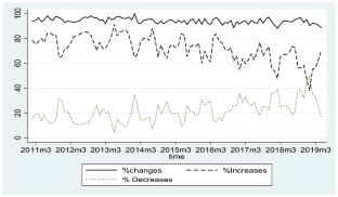
Inflation and relative price variability: new evidence from survey-based measures of inflation expectations in australia.

Inflation in India

High versus low inflation: implications for price-level convergence, data availability.

The data that support the findings of this study are openly available in Ministry of Statistics and Programme Implementation webpage at https://training.niip.gov.in/web/niip/themes-categories/-/report/view/1101 .

Aggarwal, N., & Narayanan, S. (2021). Impact of India's demonetization on domestic agricultural markets. Available at SSRN 3066042.

Alvarez, L. J., & Burriel, P. (2010). Is a Calvo price setting model consistent with individual price data? The BE journal of Macroeconomics . https://doi.org/10.2202/1935-1690.1748

Article   Google Scholar  

Alvarez, F., & Lippi, F. (2014). Price setting with menu cost for multiproduct firms. Econometrica, 82 (1), 89–135.

Alvarez, F., Le Bihan, H., & Lippi, F. (2014). Small and large price changes and the propagation of monetary shocks (No. w20155). National Bureau of Economic Research.

Alvarez, F., Le Bihan, H., & Lippi, F. (2016). The real effects of monetary shocks in sticky price models: A sufficient statistic approach. American Economic Review, 106 (10), 2817–2851.

Angeriz, A., & Arestis, P. (2007). Assessing the performance of ‘inflation targeting lite’countries. World Economy, 30 (11), 1621–1645.

Ball, L., & Sheridan, N. (2005). Does inflation targeting matter? The inflation targeting debate (pp. 249–276). University of Chicago Press.

Google Scholar  

Banerjee, A., & Kala, N. (2017). The economic and political consequences of India’s demonetisation.  VoxDev, https://voxdev.org/topic/institutions-political-economy/economic-and-political-consequences-india-s-demonetisation ,  6 .

Barros, R., Bonomo, M., Carvalho, C., & Matos, S. (2009). Price setting in a variable macroeconomic environment: Evidence from Brazilian CPI. Unpublished paper, Getulio Vargas Foundation and Federal Reserve Bank of New York.

Bernanke, B. S., Laubach, T., Mishkin, F. S., & Posen, A. S. (1999). Missing the mark-the truth about inflation targeting. Foreign Affairs, 78 , 158.

Bils, M., & Klenow, P. J. (2004). Some evidence on the importance of sticky prices. Journal of Political Economy, 112 (5), 947–985.

Bunn, P., & Ellis, C. (2009). Price-setting behaviour in the United Kingdom: a microdata approach. Bank of England Quarterly Bulletin, 49 (1), 28–36.

Bunn, P., & Ellis, C. (2012a). Examining the behaviour of individual UK consumer prices. The Economic Journal, 122 (558), F35–F55.

Bunn, P., & Ellis, C. (2012b). How do individual UK producer prices behave? The Economic Journal, 122 (558), F16–F34.

Chodorow-Reich, G., Gopinath, G., Mishra, P., & Narayanan, A. (2020). Cash and the economy: Evidence from India’s demonetization. The Quarterly Journal of Economics, 135 (1), 57–103.

Civcir, I., & Akçağlayan, A. (2010). Inflation targeting and the exchange rate: Does it matter in Turkey? Journal of Policy Modeling, 32 (3), 339–354.

Costain, J., & Nakov, A. (2011). Distributional dynamics under smoothly state-dependent pricing. Journal of Monetary Economics, 58 (6–8), 646–665.

Creel, J., & Hubert, P. (2015). Has inflation targeting changed the conduct of monetary policy? Macroeconomic Dynamics, 19 (1), 1–21.

Dhyne, E., Alvarez, L. J., Le Bihan, H., Veronese, G., Dias, D., Hoffmann, J., & Vilmunen, J. (2006). Price changes in the euro area and the United States: Some facts from individual consumer price data. Journal of Economic Perspectives, 20 (2), 171–192.

Dhyne, E., Konieczny, J., Rumler, F., & Sevestre, P. (2009). Price rigidity in the euro area-An assessment (No. 380). Directorate General Economic and Financial Affairs (DG ECFIN), European Commission.

Dixon, H. D., & Tian, K. (2017). What we can learn about the behaviour of firms from the average monthly frequency of price-changes: an application to the UK CPI data. Oxford Bulletin of Economics and Statistics, 79 (6), 907–932.

Dixon, H., Luintel, K., & Tian, K. (2020). The impact of the 2008 crisis on UK prices: What we can learn from the CPI microdata 1. Oxford Bulletin of Economics and Statistics, 82 (6), 1322–1341.

Ftiti, Z., & Hichri, W. (2014). The price stability under inflation targeting regime: An analysis with a new intermediate approach. Economic Modelling, 38 , 23–32.

Gaarder, I. B. (2009). A Survival Analysis of Consumer Prices in Norway 1975–2004 (Master's thesis).

Gagnon, E. (2009). Price setting during low and high inflation: Evidence from Mexico. The Quarterly Journal of Economics, 124 (3), 1221–1263.

Johnson, D. R. (2002). The effect of inflation targeting on the behavior of expected inflation: Evidence from an 11 country panel. Journal of monetary economics, 49 (8), 1521–1538.

Kara, E. (2015). The reset inflation puzzle and the heterogeneity in price stickiness. Journal of Monetary Economics, 76 , 29–37.

King, M. (2002). The inflation target ten years on. Available at SSRN 709004.

Kovanen, A. (2006). Why do prices in Sierra Leone change so often? A case study using micro-level price data. SSRN Electronic Journal . https://doi.org/10.2139/ssrn.892944

Krishnan, D., & Siegel, S. (2017). Effects of demonetization: Evidence from 28 slum neighborhoods in mumbai. Available at SSRN 2896026.

Lin, S., & Ye, H. (2007). Does inflation targeting really make a difference? Evaluating the treatment effect of inflation targeting in seven industrial countries. Journal of Monetary Economics, 54 (8), 2521–2533.

Medina, J. P., Rappoport, D., & Soto, C. (2007). Dynamics of price adjustments: Evidence from micro level data for Chile. Central Bank of Chile Working Paper, 432.

Midrigan, V. (2011). Menu costs, multiproduct firms, and aggregate fluctuations. Econometrica, 79 (4), 1139–1180.

Mishkin, F. S. (2000). Inflation targeting in emerging-market countries. American Economic Review, 90 (2), 105–109.

Mishkin, F. S., & Schmidt-Hebbel, K. (2007). Does inflation targeting make a difference? . NBER working paper series no. 12876.

Morandé, F., & Tejada, M. (2008). Price stickiness in emerging economies: Empirical evidence for four Latin-American countries . University of Chile.

Nakamura, E., & Steinsson, J. (2008). Five facts about prices: A reevaluation of menu cost models. The Quarterly Journal of Economics, 123 (4), 1415–1464.

Nakamura, E., Steinsson, J., Sun, P., & Villar, D. (2018). The elusive costs of inflation: Price dispersion during the US great inflation. The Quarterly Journal of Economics, 133 (4), 1933–1980.

Neumann, M. J., & Von Hagen, J. (2002). Does inflation targeting matter? (No. B 01–2002). ZEI working paper.

RBI (2017). Macroeconomic impact of demonetisation - a preliminary assessment. https://rbidocs.rbi.org.in/rdocs/Publications/PDFs/MID10031760E85BDAFEFD497193995BB1B6DBE602.PDF .

Roger, S. (2010). Inflation targeting turns 20: A growing number of countries are making a specific inflation rate the primary goal of monetary policy, with success. Finance & Development, 47 (001), 59.

Svensson, L. E. (1997). Inflation forecast targeting: Implementing and monitoring inflation targets. European Economic Review, 41 (6), 1111–1146.

Vavra, J. (2014). Inflation dynamics and time-varying volatility: New evidence and an Ss interpretation. Quarterly Journal of Economics, 129 , 215–258.

Vega, M., & Winkelried, D. (2005). Inflation targeting and inflation behavior: A successful story? International Journal of Central Banking, 1 (3), 153–175.

Vermeulen, P. (2007). Macro Price setting in the euro area: Some stylised facts from Individual Producer Price. SSRN Electronic Journal . https://doi.org/10.2139/ssrn.1694544

Wu, T. Y. (2004). Does inflation targeting reduce inflation? An analysis for the OECD industrial countries. Working papers series 83, Central Bank of Brazil, Research Department.

Zhou, P., & Dixon, H. (2019). The determinants of price rigidity in the UK: Analysis of the CPI and PPI microdata and application to macrodata modelling. The Manchester School, 87 (5), 640–677.

Download references

No funding was received for conducting this study.

Author information

Authors and affiliations.

Indian Institute of Technology Delhi, New Delhi, 110016, India

Amlendu Dubey & Juhi Lohani

You can also search for this author in PubMed   Google Scholar

Corresponding author

Correspondence to Amlendu Dubey .

Ethics declarations

Conflict of interest.

The authors report there are no competing interests to declare.

Additional information

Publisher's note.

Springer Nature remains neutral with regard to jurisdictional claims in published maps and institutional affiliations.

Tables 5 , 6 , 7 , 8 , 9 and 10

See Figs.  4 , 5 and 6

Distribution of the magnitude of price changes

Distribution of number of months between price changes per item

Distribution of size of consumer price changes and duration since previous price

Rights and permissions

Springer Nature or its licensor (e.g. a society or other partner) holds exclusive rights to this article under a publishing agreement with the author(s) or other rightsholder(s); author self-archiving of the accepted manuscript version of this article is solely governed by the terms of such publishing agreement and applicable law.

Reprints and permissions

About this article

Dubey, A., Lohani, J. Inflation targeting and price behaviour: evidence from India. Ind. Econ. Rev. 57 , 265–284 (2022). https://doi.org/10.1007/s41775-022-00148-7

Download citation

Accepted : 04 December 2022

Published : 23 December 2022

Issue Date : December 2022

DOI : https://doi.org/10.1007/s41775-022-00148-7

Share this article

Anyone you share the following link with will be able to read this content:

Sorry, a shareable link is not currently available for this article.

Provided by the Springer Nature SharedIt content-sharing initiative

• Inflation targeting
• Demonetization
• Frequency of price changes

JEL Classification

• Find a journal
• Publish with us
• Track your research

• International
• Today’s Paper
• Premium Stories
• 🗳️ Elections 2024
• Express Shorts
• Maharashtra SSC Result
• Brand Solutions

UPSC Essentials Special: Six key areas to focus from Economy for Prelims 2024

Do you find questions from economy challenging in the upsc prelims exam have a look at these 6 predictable areas which will help you to prepare the subject better..

Is Economy the toughest nut to crack for you in the GS paper of UPSC Prelims? When compared to other subjects of the UPSC Civil Services Exam, aspirants find the Indian Economy to be one of the most challenging parts of the prelims syllabus. With UPSC Prelims 2024 around the corner, let’s understand how UPSC has dealt with Economy in prelims exams in 6 predictable areas which will help you to prepare better.

Rohit Pande , our expert, talks to Manas Srivastava and shares valuable insights on key areas and predictable themes of Economy section that aspirants must know for the upcoming Prelims 2024.

About our Expert: Rohit Pande brings over a decade of experience in strategy and consulting to the world of CSE examinations. His team has helped many students clear the exam using scientific framework-driven mentorship. He keeps a keen eye on the evolving patterns of the UPSC IAS exam and the changing study habits of GenZ UPSC aspirants, enabling them with deep, actionable, and unrivaled insights.

Why do aspirants find Economy challenging for Prelims? 

Rohit Pande: Future bureaucrats should understand the fundamentals of how the Indian economy operates. Ultimately, your role is crucial in its growth and development. Naturally, Economy is a significant subject in the UPSC exam. Given its technical nature, it is an obstacle in the preparation of students, especially those from the arts background. They spend a disproportionate amount of time without tangible returns and also end up compromising other subjects.

One of the reasons is the fact that it is difficult to set boundaries in a subject like Economics. One could keep reading endlessly assuming that it is important.

There is a simple strategy. Spend more time on predictable themes and try to know as much as possible about these themes. It will give you a competitive advantage and this is all that you need to have.

Let’s discuss 6 predictable themes from Economy based on PYQ analysis that you must brush up for Prelims 2024.

Type 1: Inflation  

Inflation is USPC’s favorite topic. The expectation is you understand the implementation-level details about inflation. A basic theoretical understanding from NCERTs, core books is not enough.

Definition, indices, how it is calculated, weightage of the different components, the various governmental and non-governmental organizations associated with it. Its impact, various methods to control.

You must keep enriching your knowledge about inflation whenever it is discussed in newspapers. 

  [CSP 2020] Consider the following statements

1. The weightage of food in Consumer Price Index (CPI) is higher than that in Wholesale Price Index ( WPI ).

2. The WPI does not capture changes in the prices of services, which CPI does.

3. Reserve Bank of India has now adopted WPI as its key measure of inflation and to decide on changing the key policy rates.

Which of the statements given above is/are correct? 

(a) 1 and 2 only

(d) 1, 2 and 3

 [CSP 2013] With reference to the Indian Economy, demand-pull inflation can be caused/increased by which of the following?

1. Expansionary policies

2. Fiscal stimulus

3. Inflation-indexing wages

4. Higher purchasing power

5. Rising interest rates

Select the correct answer using the code given below. 

(a) 1, 2 and 4 only

(b) 3, 4 and 5 only

(c) 1, 2, 3 and 5 only

(d) 1, 2, 3, 4 and 5

 [CSP 2021] Which one of the following is likely to be the most inflationary in its effects? 

(a) Repayment of public debt

(b) Borrowing from the public to finance a budget deficit

(c) Borrowing from the banks to finance a budget deficit

(d) Creation of new money to finance a budget deficit

 [CSP 2022] In India, which one of the following is responsible for maintaining price stability by controlling inflation?                                                                                                                                                                               

(a) Department of Consumer Affairs

(b) Expenditure Management Commission                                                                                                                                       

(c) Financial Stability and Development Council

(d) Reserve Bank of India                                                                                                              

 [CSP 2022] With reference to the Indian economy, consider the following statements:

1. If the inflation is too high, Reserve Bank of India (RBI) is likely to buy government securities.

2. If the rupee is rapidly depreciating, RBI is likely to sell dollars in the market.

3. If interest rates in the USA or European Union were to fall, that is likely to induce RBI to buy dollars.

Which of the statements given above are correct? 

(b) 2 and 3 only

(c) 1 and 3 only

Another important point to note here is the contrast that we see in the questions on the above theme in previous years. The questions now are more difficult and detailed than they were 6-7 years back. It is evident from the questions below: 

[CSP 2013] A rise in general level of prices may be caused by

1. an increase in the money supply

2. a decrease in the aggregate level of output

3. an increase in the effective demand

Select the correct answer using the codes given below. 

(b) 1 and 2 only

(c) 2 and 3 only

 [CSP 2013] Which one of the following is likely to be the most inflationary in its effect?

(d) Creating new money to finance a budget deficit

[CSP 2013] Consider the following statements:

1. Inflation benefits the debtors.

2. Inflation benefits the bondholders.

(a) 1 only (b) 2 only

(c) Both 1 and 2 (d) Neither 1 nor 2

[CSP 2015] With reference to inflation in India, which of the following statements is correct? 

(a) Controlling the inflation in India is the responsibility of the Government of India only

(b) The Reserve Bank of India has no role in controlling the inflation

(c) Decreased money circulation helps in controlling the inflation

(d) Increased money circulation helps in controlling the inflation

Type 2: Banks   

Testing you on your awareness about the different kinds of banks/ new categories of banks seems to be UPSC’s pet peeve. If you read any news where a new bank is being discussed, you need to cover it thoroughly. Covering all the banks mentioned below should also be a fruitful exercise. 

[CSP 2021] With reference to “Urban Cooperative Banks” in India, consider the following statements:

1. They are supervised and regulated by local boards set up by the State Governments.

2. They can issue equity shares and preference shares.

3. They were brought under the purview of the Banking Regulation Act, 1949 through an Amendment in 1966.

Which of the statements given above is/are correct?

(a) 1 only (b) 2 and 3 only (c) 1 and 3only (d) 1,2 and 3

[CSP 2020] Consider the following statements:

1. In terms of short-term credit delivery to the agriculture sector, District Central Cooperative Banks (DCCBs) deliver more credit in comparison to Scheduled Commercial Banks and Regional Rural Banks.

2. One of the most important functions of DCCBs is to provide funds to the Primary Agricultural Credit Societies.

[CSP 2017] What is the purpose of setting up of Small Finance Banks (SFBs) in India?

1. To supply credit to small business units

2. To supply credit to small and marginal farmers

3. To encourage young entrepreneurs to set up business particularly in rural areas. Select the correct answer using the code given below:

(a) 1 and 2 only (b) 2 and 3 only (c) 1 and 3 only (d) 1,2 and 3

[CSP 2016]  The establishment of ‘Payment Banks’ is being allowed in India to promote financial inclusion. Which of the following statements is/are correct in this context?

1. Mobile telephone companies and supermarket chains that are owned and controlled by residents are eligible to be promoters of Payment Banks.

2. Payment Banks can issue both credit cards and debit cards.

3. Payment Banks cannot undertake lending activities.

(a) 1 and 2 only (b) 1 and 3 only (c) 2 only (d) 1, 2 and 3

[CSP 2013] Which of the following grants/grant direct credit assistance to rural households?

1. Regional Rural Banks

2. National Bank for Agriculture and Rural Development

3. Land Development Banks

(a) 1 and 2 only (b) 2 only

(c) 1 and 3 only (d) 1,2 and 3

Type 3: Banking sector measures

The Banking Sector has been in the news constantly. We want the banking sector to expand but, at the same time, adhere to regulatory measures being proposed time and again. 

[CSP 2020] What is the importance of the term “Interest Coverage Ratio” of a firm in India?

1. It helps in understanding the present risk of a firm that a bank is going to give a loan to.

2. It helps in evaluating the emerging risk of a firm that a bank is going to give a loan to.

3. The higher a borrowing firm’s level of Interest Coverage Ratio, the worse is its ability to service its debt.

Select the correct answer using the code given below:

(c) 1 and 3 only (d) 1, 2 and 3

[CSP 2019] What was the purpose of the Inter-Creditor Agreement signed by Indian banks and financial institutions recently? 

(a) To lessen to Government of India’s perennial burden of fiscal deficit and current account deficit

(b) To support the infrastructure projects of Central and State Governments

(c) To act as independent regulatory in case of applications for loans of Rs. 50 crore of more

(d) To aim at faster resolution of stressed assets of Rs. 50 crore of more which are under consortium Lending

[CSP 2018] Consider the following statements:

1. Capital Adequacy Ratio (CAR) is the amount that banks have to maintain in the form of their own funds to offset any loss that banks incur if the account-holders fail to repay dues.

2. CAR is decided by each individual bank.

Type 4: Bonds 

Bonds as Financial Instruments are UPSC’s favorites. Any new bond in the news should trigger an alert. 

[CSP 2022] With reference to the Indian economy, what are the advantages of “Inflation-Indexed Bonds (IIBs)”?

1. Government can reduce the coupon rates on its borrowing by way of IIBs.

2. IIGs provide protection to the investors from uncertainty regarding inflation. 3. The interest received as well as capital gains on IIBs are not taxable.

(a) 1 and 2 only (b) 2 and 3 only

[CSP 2022] With reference to Convertible Bonds, consider pin the following statements:

1. As there is an option to exchange the bond for equity, Convertible Bonds pay a lower rate of interest.

2. The option to convert to equity affords the bondholder a degree of indexation to rising consumer prices.

[CSP 2021] Indian Government Bond Yields are influenced by which of the following?

1. Actions of the United States Federal Reserve

2. Actions of the Reserve Bank of India

3. Inflation and short-term interest rates

(a) 1 and 2 only     (b) 2 only

(c) 3 only                (d) 1,2 and 3

[CSP 2016] What is/are the purpose/purposes of Government’s Sovereign Gold Bond Scheme’ and ‘Gold Monetization Scheme’?

1. To bring the idle gold lying with Indian households into the economy.

2. To promote FDI in the gold and jewellery sector.

3. To reduce India’s dependence on gold imports.

Select the correct answer using the code given below.:

(a) 1 only (b) 2 and 3 only (c) 1 and 3 only (d) 1,2 and 3

[CSP 2016] With reference to ‘IFC Masala Bonds’, sometimes seen in the news, which of the statements given below is/ are correct?

1. The International Finance Corporation, which offers these bonds, is an arm of the World Bank.

2. They are the rupee-denominated bonds and are a source of debt financing for the public and private sector.

(a) 1 only              (b) 2 only

(c) Both 1 and 2  (d) Neither 1 nor 2

Type 5: Taxes 

Perhaps because Revenue Officers are selected through this exam, taxes are an important theme. So, different kinds of taxes, their relationship with GDP etc. – everything matters! 

[CSP 2018] Consider the following items:

1. Cereal grains hulled

2. Chicken eggs cooked

3. Fish processed and canned

4. Newspapers containing advertising material

Which of the above items is/are exempted under GST (Goods and Services Tax)? 

(a) 1 only (b) 2 and 3 only

(c) 1, 2 and 4 only (d) 1, 2, 3 and 4

Consider the following:

1. Demographic performance

2. Forest and ecology

3. Governance reforms

4. Stable government

5. Tax and fiscal efforts

[CSP 2023] For the horizontal tax devolution, the Fifteenth Finance Commission used how many of the above as criteria other than population area and income distance? (2023)

(a) Only two (b) Only three

(c) Only four (d) All five

[CSP 2018] With reference to India’s decision to levy an equalization tax of 6% on online advertisement services offered by non-resident entities, which of the following statements is/are correct?

1. It is introduced as a part of the Income Tax Act.

2. Non-resident entities that offer advertisement services in India can claim a tax credit in their home country under the “Double Taxation Avoidance Agreements”.

Select the correct answer using the code given below: 

(a) 1 only             (b) 2 only

[CSP 2017] What is/are the most likely advantages of implementing ‘Goods and Services Tax (GST)’?

1. It will replace multiple taxes collected by multiple authorities and will thus create a single market in India.

2. It will drastically reduce the ‘Current Account Deficit’ of India and will enable it to increase its foreign exchange reserves.

3. It will enormously increase the growth and size of economy of India and will enable it to overtake China in the near future.

(a) 1 only (b) 2 and 3 only (c) 1 and 3 only (d) 1, 2 and 3

[CSP 2015] A decrease in the tax-to-GDP ratio of a country indicates which of the following?

1. Slowing economic growth rate.

2. Less equitable distribution of national income.

Select the correct answer using the code given below.

[CSP 2014] The sales tax you pay while purchasing a toothpaste is a 

(a) tax imposed by the Central Government

(b) tax imposed by the Central Government but collected by the State Government

(c) tax imposed by the State Government but collected by the Central Government

(d) tax imposed and collected by the State Government

[CSP 2017] Consider the following statements:

1. Tax revenue as a percent of GDP of India has steadily increased in the last decade.

2. Fiscal deficit as a percent of GDP of India has steadily increased in the last decade. Which of the statements given above is/are correct?

Type 6: Trade  

We live in a globalized world. A deep understanding of how our economy and global economy are intertwined is important.   So when UPSC asks questions related to trade, themes and topics like Exports, FDI, BoP, etc. become important. 

[CSP 2023] Consider the following statement:

Statement I:

India accounts for 3.2% of global export of goods.

Statement II:

Many local companies and some foreign companies operating in India have taken advantage of India’s ‘Production-linked Incentive’ scheme.

Which one of the following is correct in respect of the above statements? 

(a) Both statement-I and Statement II are correct and Statement II is the correct explanation for

Statement-I

(b) Both Statement-I and Statement-II are correct and Statement-II is not the correct explanation

for Statement-I

(c) Statement-I is correct but Statement-II is incorrect

(d) Statement-I- is incorrect but Statement-II is correct

[CSP 2021] With reference to Foreign Direct Investment in India, which one of the following is considered its major characteristic? 

(a) It is the investment through capitol instruments essentially in a listed company.

(b) It is largely non-debt creating capital flow.

(c) It is the investment which involves debt-servicing.

(d) It is the investment made by foreign institutional investors in the Government securities.

[CSP 2020] With reference to Trade-Related Investment Measures (TRIMS), which of the following statements is/are correct?

1. Quantitative restrictions on imports by foreign investors are prohibited.

2. They apply to investment measures related to trade in both goods and services.

3. They are not concerned with the regulation of foreign investment.

1. The value of Indo-Sri Lanka trade has consistently increased in the last decade.

2. “Textile and textile articles” constitute an important item of the trade between India and Bangladesh.

3. In the last five years, Nepal has been the largest trading partner of India in South Asia. Which of the statements given above is/are correct? (2020)

(a) 1 and 2 only  (b) 2 only

(c) 3 only      (d) 1, 2 and 3

[CSP 2020] With reference to the international trade of India at present, which of the following statements is/are correct?

1. India’s merchandise exports are less than its merchandise imports.

2. India’s imports of iron and steel, chemicals, fertilisers and machinery have decreased in recent years.

3. India’s exports of services are more than its imports of services.

4. India suffers from an overall trade/current account deficit. Select the correct answer using the code given below:

(a) 1 and 2 only (b) 2 and 4 only

(c) 3 only           (d) 1, 3 and 4 only

[CSP 2019] Among the agricultural commodities imported by India, which one of the following accounts for the highest imports in terms of value in the last five years?

(a) Spices (b) Fresh fruits

(c) Pulses (d) Vegetable oils

Within this theme, the questions being asked 5-7 years back were simpler. Have a look:

[CSP 2014] With reference to Balance of Payments, which of the following constitutes/constitute the Current Account?

1. Balance of trade

2. Foreign assets

3. Balance of invisibles

4. Special Drawing Rights Select the correct answer using the code given below. (2014)

(a) 1 only (b) 2 and 3

(c) 1 and 3 (d) 1, 2 and 4

[CSP 2013] The balance of payments of a country is a systematic record of 

(a) all import and export transactions of a country during a given period of time, normally a year

(b) good exported from a country during a year

(c) economic transaction between the government of one country to another

(d) capital movements from one country to another.

[CSP 2013] Which of the following constitute Capital Account?

1. Foreign Loans

2. Foreign Direct Investment

3. Private Remittances

4. Portfolio Investment

Select the correct answer using the codes given below.

(a) 1, 2 and 3 (b) 1, 2 and 4

(c) 2,3 and 4 (d) 1, 3 and 4

EXPERT’S ADVICE: 

No doubt, questions from Economics are on the tougher side. Being well prepared with PYQs will ensure you have some idea about some options and that you are in a position to take a leap of faith, make intelligent guesses. 

Subscribe to our  UPSC newsletter  and stay updated with the news cues from the past week.

The UPSC articles of  Indian Express is now on Telegram. Join our Telegram channel- Indian Express UPSC Hub and stay updated with the latest Updates.

Manas Srivastava is currently working as Deputy Copy Editor with The Indian Express (digital) and majorly writes for UPSC-related projects leading a unique initiative known as UPSC Essentials. In the past, Manas has represented India at the G-20 Youth Summit in Mexico. He is a former member of the Youth Council, GOI. A two-time topper/gold medallist in History (both in graduation and post-graduation) from Delhi University, he has mentored and taught UPSC aspirants for more than four years. His diverse role in The Indian Express consists of writing, editing, anchoring/ hosting, interviewing experts, and curating and simplifying news for the benefit of students. He hosts the YouTube talk show called ‘Art and Culture with Devdutt Pattanaik’ and a LIVE series on Instagram and YouTube called ‘You Ask We Answer’.His talks on ‘How to read a newspaper’ focus on newspaper reading as an essential habit for students. His articles and videos aim at finding solutions to the general queries of students and hence he believes in being students' editor, preparing them not just for any exam but helping them to become informed citizens. This is where he makes his teaching profession meet journalism. He is also currently working on a monthly magazine for UPSC Aspirants. He is a recipient of the Dip Chand Memorial Award, the Lala Ram Mohan Prize and Prof. Papiya Ghosh Memorial Prize for academic excellence. He was also awarded the University’s Post-Graduate Scholarship for pursuing M.A. in History where he chose to specialise in Ancient India due to his keen interest in Archaeology. He has also successfully completed a Certificate course on Women’s Studies by the Women’s Studies Development Centre, DU. As a part of N.S.S in the past, Manas has worked with national and international organisations and has shown keen interest and active participation in Social Service. He has led and been a part of projects involving areas such as gender sensitisation, persons with disability, helping slum dwellers, environment, adopting our heritage programme. He has also presented a case study on ‘Psychological stress among students’ at ICSQCC- Sri Lanka. As a compere for seminars and other events he likes to keep his orating hobby alive. His interests also lie in International Relations, Governance, Social issues, Essays and poetry. ... Read More

• government jobs
• Sarkari Naukri
• UPSC Civil Services
• UPSC Civil Services Exam
• UPSC Essentials
• UPSC Specials

Maharashtra SSC result 2024 has been declared with an overall pass percentage of 95.81%. The Konkan district has the highest pass percentage while Nagpur has the lowest. Out of 23288 registered schools, 9382 recorded a 100% result. Students can apply for re-evaluation or grade-improvement exams from May 28 to June 11.

UPSC Magazine

Read UPSC Magazine

• Cyclone Remal Live Updates: Severe cyclonic storm claims six lives in West Bengal, 8 Kolkata-bound flights diverted 3 hours ago
• Maharashtra SSC 10th Result 2024 Live Updates: Result out, revaluation application to begin from May 28 3 hours ago
• Maharashtra SSC 10th Results 2024 Live Updates: 95.81% pass, grade improvement application from May 31 onwards 3 hours ago
• JEE Advanced 2024 Live Updates: Check last five year cut offs 3 hours ago

Best of Express

Buzzing Now

May 27: Latest News

• 01 Bangladesh MP killing: Dhaka police team arrives in city, says trying to trace accused businessman via Interpol
• 02 Armenians throng center of the capital to demand the prime minister’s resignation
• 03 Ghatkopar billboard collapse: Hoarding pillars a few feet deep, poor quality work for financial benefits, say police
• 04 Macron heads to Germany in first French presidential state visit in 24 years
• 05 IPL final: KKR runaway winner as near perfect script unfolds at Chennai
• Elections 2024
• Political Pulse
• Entertainment
• Movie Review
• Newsletters
• Web Stories

• Work & Careers
• Life & Arts

Become an FT subscriber

Try unlimited access Only $1 for 4 weeks

Then $75 per month. Complete digital access to quality FT journalism on any device. Cancel anytime during your trial.

• Global news & analysis
• Expert opinion
• Special features
• FirstFT newsletter
• Videos & Podcasts
• Android & iOS app
• FT Edit app
• 10 gift articles per month

Explore more offers.

Standard digital.

• FT Digital Edition

Premium Digital

Print + premium digital, ft professional, weekend print + standard digital, weekend print + premium digital.

Essential digital access to quality FT journalism on any device. Pay a year upfront and save 20%.

• Global news & analysis
• Exclusive FT analysis
• FT App on Android & iOS
• FirstFT: the day's biggest stories
• 20+ curated newsletters
• Follow topics & set alerts with myFT
• FT Videos & Podcasts
• 20 monthly gift articles to share
• Lex: FT's flagship investment column
• 15+ Premium newsletters by leading experts
• FT Digital Edition: our digitised print edition
• Weekday Print Edition
• Videos & Podcasts
• Premium newsletters
• 10 additional gift articles per month
• FT Weekend Print delivery
• Everything in Standard Digital
• Everything in Premium Digital

Complete digital access to quality FT journalism with expert analysis from industry leaders. Pay a year upfront and save 20%.

• 10 monthly gift articles to share
• Everything in Print
• Make and share highlights
• FT Workspace
• Markets data widget
• Subscription Manager
• Workflow integrations
• Occasional readers go free
• Volume discount

Terms & Conditions apply

Explore our full range of subscriptions.

Why the ft.

See why over a million readers pay to read the Financial Times.

International Edition

Sathyanarayanan Ramachandran to Deliver a Presentation at ADMC 2024, Delft, Netherlands

The paper  Design Thinking View on an affordable public bike-sharing project from India  by Sathyanarayanan Ramachandran, Associate Professor of Marketing, IFMR Graduate School of Business, Krea University, has been accepted for presentation at the  Academic Design Management Conference (ADMC) 2024. 

ADMC is a prestigious international academic design management conference held annually in various locations around the world. This year, it will take place in Delft, Netherlands. Sathyanarayanan Ramachandran will present his paper on 6-7 August, 2024.

Discover Krea

In other news, dr gayathri sampath authors a short story titled pest control, does cap-and-trade scheme impact energy efficiency and firm value empirical evidence from india, sathyanarayanan ramachandran delivers a talk on marketing success case studies in the organic products industry, ivey case website publishes a case by dr pallavi pandey, ifmr gsb - krea university.