introduction of presentation and data response

Home Blog Design Understanding Data Presentations (Guide + Examples)

Understanding Data Presentations (Guide + Examples)

In this age of overwhelming information, the skill to effectively convey data has become extremely valuable. Initiating a discussion on data presentation types involves thoughtful consideration of the nature of your data and the message you aim to convey. Different types of visualizations serve distinct purposes. Whether you’re dealing with how to develop a report or simply trying to communicate complex information, how you present data influences how well your audience understands and engages with it. This extensive guide leads you through the different ways of data presentation.

Table of Contents

What is a Data Presentation?

What should a data presentation include, line graphs, treemap chart, scatter plot, how to choose a data presentation type, recommended data presentation templates, common mistakes done in data presentation.

A data presentation is a slide deck that aims to disclose quantitative information to an audience through the use of visual formats and narrative techniques derived from data analysis, making complex data understandable and actionable. This process requires a series of tools, such as charts, graphs, tables, infographics, dashboards, and so on, supported by concise textual explanations to improve understanding and boost retention rate.

Data presentations require us to cull data in a format that allows the presenter to highlight trends, patterns, and insights so that the audience can act upon the shared information. In a few words, the goal of data presentations is to enable viewers to grasp complicated concepts or trends quickly, facilitating informed decision-making or deeper analysis.

Data presentations go beyond the mere usage of graphical elements. Seasoned presenters encompass visuals with the art of storytelling with data, so the speech skillfully connects the points through a narrative that resonates with the audience. Depending on the purpose – inspire, persuade, inform, support decision-making processes, etc. – is the data presentation format that is better suited to help us in this journey.

To nail your upcoming data presentation, ensure to count with the following elements:

• Clear Objectives: Understand the intent of your presentation before selecting the graphical layout and metaphors to make content easier to grasp.
• Engaging introduction: Use a powerful hook from the get-go. For instance, you can ask a big question or present a problem that your data will answer. Take a look at our guide on how to start a presentation for tips & insights.
• Structured Narrative: Your data presentation must tell a coherent story. This means a beginning where you present the context, a middle section in which you present the data, and an ending that uses a call-to-action. Check our guide on presentation structure for further information.
• Visual Elements: These are the charts, graphs, and other elements of visual communication we ought to use to present data. This article will cover one by one the different types of data representation methods we can use, and provide further guidance on choosing between them.
• Insights and Analysis: This is not just showcasing a graph and letting people get an idea about it. A proper data presentation includes the interpretation of that data, the reason why it’s included, and why it matters to your research.
• Conclusion & CTA: Ending your presentation with a call to action is necessary. Whether you intend to wow your audience into acquiring your services, inspire them to change the world, or whatever the purpose of your presentation, there must be a stage in which you convey all that you shared and show the path to staying in touch. Plan ahead whether you want to use a thank-you slide, a video presentation, or which method is apt and tailored to the kind of presentation you deliver.
• Q&A Session: After your speech is concluded, allocate 3-5 minutes for the audience to raise any questions about the information you disclosed. This is an extra chance to establish your authority on the topic. Check our guide on questions and answer sessions in presentations here.

Bar charts are a graphical representation of data using rectangular bars to show quantities or frequencies in an established category. They make it easy for readers to spot patterns or trends. Bar charts can be horizontal or vertical, although the vertical format is commonly known as a column chart. They display categorical, discrete, or continuous variables grouped in class intervals [1] . They include an axis and a set of labeled bars horizontally or vertically. These bars represent the frequencies of variable values or the values themselves. Numbers on the y-axis of a vertical bar chart or the x-axis of a horizontal bar chart are called the scale.

Real-Life Application of Bar Charts

Let’s say a sales manager is presenting sales to their audience. Using a bar chart, he follows these steps.

Step 1: Selecting Data

The first step is to identify the specific data you will present to your audience.

The sales manager has highlighted these products for the presentation.

• Product A: Men’s Shoes
• Product B: Women’s Apparel
• Product C: Electronics
• Product D: Home Decor

Step 2: Choosing Orientation

Opt for a vertical layout for simplicity. Vertical bar charts help compare different categories in case there are not too many categories [1] . They can also help show different trends. A vertical bar chart is used where each bar represents one of the four chosen products. After plotting the data, it is seen that the height of each bar directly represents the sales performance of the respective product.

It is visible that the tallest bar (Electronics – Product C) is showing the highest sales. However, the shorter bars (Women’s Apparel – Product B and Home Decor – Product D) need attention. It indicates areas that require further analysis or strategies for improvement.

Step 3: Colorful Insights

Different colors are used to differentiate each product. It is essential to show a color-coded chart where the audience can distinguish between products.

• Men’s Shoes (Product A): Yellow
• Women’s Apparel (Product B): Orange
• Electronics (Product C): Violet
• Home Decor (Product D): Blue

Bar charts are straightforward and easily understandable for presenting data. They are versatile when comparing products or any categorical data [2] . Bar charts adapt seamlessly to retail scenarios. Despite that, bar charts have a few shortcomings. They cannot illustrate data trends over time. Besides, overloading the chart with numerous products can lead to visual clutter, diminishing its effectiveness.

For more information, check our collection of bar chart templates for PowerPoint .

Line graphs help illustrate data trends, progressions, or fluctuations by connecting a series of data points called ‘markers’ with straight line segments. This provides a straightforward representation of how values change [5] . Their versatility makes them invaluable for scenarios requiring a visual understanding of continuous data. In addition, line graphs are also useful for comparing multiple datasets over the same timeline. Using multiple line graphs allows us to compare more than one data set. They simplify complex information so the audience can quickly grasp the ups and downs of values. From tracking stock prices to analyzing experimental results, you can use line graphs to show how data changes over a continuous timeline. They show trends with simplicity and clarity.

Real-life Application of Line Graphs

To understand line graphs thoroughly, we will use a real case. Imagine you’re a financial analyst presenting a tech company’s monthly sales for a licensed product over the past year. Investors want insights into sales behavior by month, how market trends may have influenced sales performance and reception to the new pricing strategy. To present data via a line graph, you will complete these steps.

First, you need to gather the data. In this case, your data will be the sales numbers. For example:

• January: $45,000
• February: $55,000
• March: $45,000
• April: $60,000
• May: $ 70,000
• June: $65,000
• July: $62,000
• August: $68,000
• September: $81,000
• October: $76,000
• November: $87,000
• December: $91,000

After choosing the data, the next step is to select the orientation. Like bar charts, you can use vertical or horizontal line graphs. However, we want to keep this simple, so we will keep the timeline (x-axis) horizontal while the sales numbers (y-axis) vertical.

Step 3: Connecting Trends

After adding the data to your preferred software, you will plot a line graph. In the graph, each month’s sales are represented by data points connected by a line.

Step 4: Adding Clarity with Color

If there are multiple lines, you can also add colors to highlight each one, making it easier to follow.

Line graphs excel at visually presenting trends over time. These presentation aids identify patterns, like upward or downward trends. However, too many data points can clutter the graph, making it harder to interpret. Line graphs work best with continuous data but are not suitable for categories.

For more information, check our collection of line chart templates for PowerPoint and our article about how to make a presentation graph .

A data dashboard is a visual tool for analyzing information. Different graphs, charts, and tables are consolidated in a layout to showcase the information required to achieve one or more objectives. Dashboards help quickly see Key Performance Indicators (KPIs). You don’t make new visuals in the dashboard; instead, you use it to display visuals you’ve already made in worksheets [3] .

Keeping the number of visuals on a dashboard to three or four is recommended. Adding too many can make it hard to see the main points [4]. Dashboards can be used for business analytics to analyze sales, revenue, and marketing metrics at a time. They are also used in the manufacturing industry, as they allow users to grasp the entire production scenario at the moment while tracking the core KPIs for each line.

Real-Life Application of a Dashboard

Consider a project manager presenting a software development project’s progress to a tech company’s leadership team. He follows the following steps.

Step 1: Defining Key Metrics

To effectively communicate the project’s status, identify key metrics such as completion status, budget, and bug resolution rates. Then, choose measurable metrics aligned with project objectives.

Step 2: Choosing Visualization Widgets

After finalizing the data, presentation aids that align with each metric are selected. For this project, the project manager chooses a progress bar for the completion status and uses bar charts for budget allocation. Likewise, he implements line charts for bug resolution rates.

Step 3: Dashboard Layout

Key metrics are prominently placed in the dashboard for easy visibility, and the manager ensures that it appears clean and organized.

Dashboards provide a comprehensive view of key project metrics. Users can interact with data, customize views, and drill down for detailed analysis. However, creating an effective dashboard requires careful planning to avoid clutter. Besides, dashboards rely on the availability and accuracy of underlying data sources.

For more information, check our article on how to design a dashboard presentation , and discover our collection of dashboard PowerPoint templates .

Treemap charts represent hierarchical data structured in a series of nested rectangles [6] . As each branch of the ‘tree’ is given a rectangle, smaller tiles can be seen representing sub-branches, meaning elements on a lower hierarchical level than the parent rectangle. Each one of those rectangular nodes is built by representing an area proportional to the specified data dimension.

Treemaps are useful for visualizing large datasets in compact space. It is easy to identify patterns, such as which categories are dominant. Common applications of the treemap chart are seen in the IT industry, such as resource allocation, disk space management, website analytics, etc. Also, they can be used in multiple industries like healthcare data analysis, market share across different product categories, or even in finance to visualize portfolios.

Real-Life Application of a Treemap Chart

Let’s consider a financial scenario where a financial team wants to represent the budget allocation of a company. There is a hierarchy in the process, so it is helpful to use a treemap chart. In the chart, the top-level rectangle could represent the total budget, and it would be subdivided into smaller rectangles, each denoting a specific department. Further subdivisions within these smaller rectangles might represent individual projects or cost categories.

Step 1: Define Your Data Hierarchy

While presenting data on the budget allocation, start by outlining the hierarchical structure. The sequence will be like the overall budget at the top, followed by departments, projects within each department, and finally, individual cost categories for each project.

• Top-level rectangle: Total Budget
• Second-level rectangles: Departments (Engineering, Marketing, Sales)
• Third-level rectangles: Projects within each department
• Fourth-level rectangles: Cost categories for each project (Personnel, Marketing Expenses, Equipment)

Step 2: Choose a Suitable Tool

It’s time to select a data visualization tool supporting Treemaps. Popular choices include Tableau, Microsoft Power BI, PowerPoint, or even coding with libraries like D3.js. It is vital to ensure that the chosen tool provides customization options for colors, labels, and hierarchical structures.

Here, the team uses PowerPoint for this guide because of its user-friendly interface and robust Treemap capabilities.

Step 3: Make a Treemap Chart with PowerPoint

After opening the PowerPoint presentation, they chose “SmartArt” to form the chart. The SmartArt Graphic window has a “Hierarchy” category on the left.  Here, you will see multiple options. You can choose any layout that resembles a Treemap. The “Table Hierarchy” or “Organization Chart” options can be adapted. The team selects the Table Hierarchy as it looks close to a Treemap.

Step 5: Input Your Data

After that, a new window will open with a basic structure. They add the data one by one by clicking on the text boxes. They start with the top-level rectangle, representing the total budget.  

Step 6: Customize the Treemap

By clicking on each shape, they customize its color, size, and label. At the same time, they can adjust the font size, style, and color of labels by using the options in the “Format” tab in PowerPoint. Using different colors for each level enhances the visual difference.

Treemaps excel at illustrating hierarchical structures. These charts make it easy to understand relationships and dependencies. They efficiently use space, compactly displaying a large amount of data, reducing the need for excessive scrolling or navigation. Additionally, using colors enhances the understanding of data by representing different variables or categories.

In some cases, treemaps might become complex, especially with deep hierarchies.  It becomes challenging for some users to interpret the chart. At the same time, displaying detailed information within each rectangle might be constrained by space. It potentially limits the amount of data that can be shown clearly. Without proper labeling and color coding, there’s a risk of misinterpretation.

A heatmap is a data visualization tool that uses color coding to represent values across a two-dimensional surface. In these, colors replace numbers to indicate the magnitude of each cell. This color-shaded matrix display is valuable for summarizing and understanding data sets with a glance [7] . The intensity of the color corresponds to the value it represents, making it easy to identify patterns, trends, and variations in the data.

As a tool, heatmaps help businesses analyze website interactions, revealing user behavior patterns and preferences to enhance overall user experience. In addition, companies use heatmaps to assess content engagement, identifying popular sections and areas of improvement for more effective communication. They excel at highlighting patterns and trends in large datasets, making it easy to identify areas of interest.

We can implement heatmaps to express multiple data types, such as numerical values, percentages, or even categorical data. Heatmaps help us easily spot areas with lots of activity, making them helpful in figuring out clusters [8] . When making these maps, it is important to pick colors carefully. The colors need to show the differences between groups or levels of something. And it is good to use colors that people with colorblindness can easily see.

Check our detailed guide on how to create a heatmap here. Also discover our collection of heatmap PowerPoint templates .

Pie charts are circular statistical graphics divided into slices to illustrate numerical proportions. Each slice represents a proportionate part of the whole, making it easy to visualize the contribution of each component to the total.

The size of the pie charts is influenced by the value of data points within each pie. The total of all data points in a pie determines its size. The pie with the highest data points appears as the largest, whereas the others are proportionally smaller. However, you can present all pies of the same size if proportional representation is not required [9] . Sometimes, pie charts are difficult to read, or additional information is required. A variation of this tool can be used instead, known as the donut chart , which has the same structure but a blank center, creating a ring shape. Presenters can add extra information, and the ring shape helps to declutter the graph.

Pie charts are used in business to show percentage distribution, compare relative sizes of categories, or present straightforward data sets where visualizing ratios is essential.

Real-Life Application of Pie Charts

Consider a scenario where you want to represent the distribution of the data. Each slice of the pie chart would represent a different category, and the size of each slice would indicate the percentage of the total portion allocated to that category.

Step 1: Define Your Data Structure

Imagine you are presenting the distribution of a project budget among different expense categories.

• Column A: Expense Categories (Personnel, Equipment, Marketing, Miscellaneous)
• Column B: Budget Amounts ($40,000, $30,000, $20,000, $10,000) Column B represents the values of your categories in Column A.

Step 2: Insert a Pie Chart

Using any of the accessible tools, you can create a pie chart. The most convenient tools for forming a pie chart in a presentation are presentation tools such as PowerPoint or Google Slides.  You will notice that the pie chart assigns each expense category a percentage of the total budget by dividing it by the total budget.

For instance:

• Personnel: $40,000 / ($40,000 + $30,000 + $20,000 + $10,000) = 40%
• Equipment: $30,000 / ($40,000 + $30,000 + $20,000 + $10,000) = 30%
• Marketing: $20,000 / ($40,000 + $30,000 + $20,000 + $10,000) = 20%
• Miscellaneous: $10,000 / ($40,000 + $30,000 + $20,000 + $10,000) = 10%

You can make a chart out of this or just pull out the pie chart from the data.

3D pie charts and 3D donut charts are quite popular among the audience. They stand out as visual elements in any presentation slide, so let’s take a look at how our pie chart example would look in 3D pie chart format.

Step 03: Results Interpretation

The pie chart visually illustrates the distribution of the project budget among different expense categories. Personnel constitutes the largest portion at 40%, followed by equipment at 30%, marketing at 20%, and miscellaneous at 10%. This breakdown provides a clear overview of where the project funds are allocated, which helps in informed decision-making and resource management. It is evident that personnel are a significant investment, emphasizing their importance in the overall project budget.

Pie charts provide a straightforward way to represent proportions and percentages. They are easy to understand, even for individuals with limited data analysis experience. These charts work well for small datasets with a limited number of categories.

However, a pie chart can become cluttered and less effective in situations with many categories. Accurate interpretation may be challenging, especially when dealing with slight differences in slice sizes. In addition, these charts are static and do not effectively convey trends over time.

For more information, check our collection of pie chart templates for PowerPoint .

Histograms present the distribution of numerical variables. Unlike a bar chart that records each unique response separately, histograms organize numeric responses into bins and show the frequency of reactions within each bin [10] . The x-axis of a histogram shows the range of values for a numeric variable. At the same time, the y-axis indicates the relative frequencies (percentage of the total counts) for that range of values.

Whenever you want to understand the distribution of your data, check which values are more common, or identify outliers, histograms are your go-to. Think of them as a spotlight on the story your data is telling. A histogram can provide a quick and insightful overview if you’re curious about exam scores, sales figures, or any numerical data distribution.

Real-Life Application of a Histogram

In the histogram data analysis presentation example, imagine an instructor analyzing a class’s grades to identify the most common score range. A histogram could effectively display the distribution. It will show whether most students scored in the average range or if there are significant outliers.

Step 1: Gather Data

He begins by gathering the data. The scores of each student in class are gathered to analyze exam scores.

After arranging the scores in ascending order, bin ranges are set.

Step 2: Define Bins

Bins are like categories that group similar values. Think of them as buckets that organize your data. The presenter decides how wide each bin should be based on the range of the values. For instance, the instructor sets the bin ranges based on score intervals: 60-69, 70-79, 80-89, and 90-100.

Step 3: Count Frequency

Now, he counts how many data points fall into each bin. This step is crucial because it tells you how often specific ranges of values occur. The result is the frequency distribution, showing the occurrences of each group.

Here, the instructor counts the number of students in each category.

• 60-69: 1 student (Kate)
• 70-79: 4 students (David, Emma, Grace, Jack)
• 80-89: 7 students (Alice, Bob, Frank, Isabel, Liam, Mia, Noah)
• 90-100: 3 students (Clara, Henry, Olivia)

Step 4: Create the Histogram

It’s time to turn the data into a visual representation. Draw a bar for each bin on a graph. The width of the bar should correspond to the range of the bin, and the height should correspond to the frequency.  To make your histogram understandable, label the X and Y axes.

In this case, the X-axis should represent the bins (e.g., test score ranges), and the Y-axis represents the frequency.

The histogram of the class grades reveals insightful patterns in the distribution. Most students, with seven students, fall within the 80-89 score range. The histogram provides a clear visualization of the class’s performance. It showcases a concentration of grades in the upper-middle range with few outliers at both ends. This analysis helps in understanding the overall academic standing of the class. It also identifies the areas for potential improvement or recognition.

Thus, histograms provide a clear visual representation of data distribution. They are easy to interpret, even for those without a statistical background. They apply to various types of data, including continuous and discrete variables. One weak point is that histograms do not capture detailed patterns in students’ data, with seven compared to other visualization methods.

A scatter plot is a graphical representation of the relationship between two variables. It consists of individual data points on a two-dimensional plane. This plane plots one variable on the x-axis and the other on the y-axis. Each point represents a unique observation. It visualizes patterns, trends, or correlations between the two variables.

Scatter plots are also effective in revealing the strength and direction of relationships. They identify outliers and assess the overall distribution of data points. The points’ dispersion and clustering reflect the relationship’s nature, whether it is positive, negative, or lacks a discernible pattern. In business, scatter plots assess relationships between variables such as marketing cost and sales revenue. They help present data correlations and decision-making.

Real-Life Application of Scatter Plot

A group of scientists is conducting a study on the relationship between daily hours of screen time and sleep quality. After reviewing the data, they managed to create this table to help them build a scatter plot graph:

In the provided example, the x-axis represents Daily Hours of Screen Time, and the y-axis represents the Sleep Quality Rating.

The scientists observe a negative correlation between the amount of screen time and the quality of sleep. This is consistent with their hypothesis that blue light, especially before bedtime, has a significant impact on sleep quality and metabolic processes.

There are a few things to remember when using a scatter plot. Even when a scatter diagram indicates a relationship, it doesn’t mean one variable affects the other. A third factor can influence both variables. The more the plot resembles a straight line, the stronger the relationship is perceived [11] . If it suggests no ties, the observed pattern might be due to random fluctuations in data. When the scatter diagram depicts no correlation, whether the data might be stratified is worth considering.

Choosing the appropriate data presentation type is crucial when making a presentation . Understanding the nature of your data and the message you intend to convey will guide this selection process. For instance, when showcasing quantitative relationships, scatter plots become instrumental in revealing correlations between variables. If the focus is on emphasizing parts of a whole, pie charts offer a concise display of proportions. Histograms, on the other hand, prove valuable for illustrating distributions and frequency patterns. 

Bar charts provide a clear visual comparison of different categories. Likewise, line charts excel in showcasing trends over time, while tables are ideal for detailed data examination. Starting a presentation on data presentation types involves evaluating the specific information you want to communicate and selecting the format that aligns with your message. This ensures clarity and resonance with your audience from the beginning of your presentation.

1. Fact Sheet Dashboard for Data Presentation

Convey all the data you need to present in this one-pager format, an ideal solution tailored for users looking for presentation aids. Global maps, donut chats, column graphs, and text neatly arranged in a clean layout presented in light and dark themes.

Use This Template

2. 3D Column Chart Infographic PPT Template

Represent column charts in a highly visual 3D format with this PPT template. A creative way to present data, this template is entirely editable, and we can craft either a one-page infographic or a series of slides explaining what we intend to disclose point by point.

3. Data Circles Infographic PowerPoint Template

An alternative to the pie chart and donut chart diagrams, this template features a series of curved shapes with bubble callouts as ways of presenting data. Expand the information for each arch in the text placeholder areas.

4. Colorful Metrics Dashboard for Data Presentation

This versatile dashboard template helps us in the presentation of the data by offering several graphs and methods to convert numbers into graphics. Implement it for e-commerce projects, financial projections, project development, and more.

5. Animated Data Presentation Tools for PowerPoint & Google Slides

A slide deck filled with most of the tools mentioned in this article, from bar charts, column charts, treemap graphs, pie charts, histogram, etc. Animated effects make each slide look dynamic when sharing data with stakeholders.

6. Statistics Waffle Charts PPT Template for Data Presentations

This PPT template helps us how to present data beyond the typical pie chart representation. It is widely used for demographics, so it’s a great fit for marketing teams, data science professionals, HR personnel, and more.

7. Data Presentation Dashboard Template for Google Slides

A compendium of tools in dashboard format featuring line graphs, bar charts, column charts, and neatly arranged placeholder text areas. 

8. Weather Dashboard for Data Presentation

Share weather data for agricultural presentation topics, environmental studies, or any kind of presentation that requires a highly visual layout for weather forecasting on a single day. Two color themes are available.

9. Social Media Marketing Dashboard Data Presentation Template

Intended for marketing professionals, this dashboard template for data presentation is a tool for presenting data analytics from social media channels. Two slide layouts featuring line graphs and column charts.

10. Project Management Summary Dashboard Template

A tool crafted for project managers to deliver highly visual reports on a project’s completion, the profits it delivered for the company, and expenses/time required to execute it. 4 different color layouts are available.

11. Profit & Loss Dashboard for PowerPoint and Google Slides

A must-have for finance professionals. This typical profit & loss dashboard includes progress bars, donut charts, column charts, line graphs, and everything that’s required to deliver a comprehensive report about a company’s financial situation.

Overwhelming visuals

One of the mistakes related to using data-presenting methods is including too much data or using overly complex visualizations. They can confuse the audience and dilute the key message.

Inappropriate chart types

Choosing the wrong type of chart for the data at hand can lead to misinterpretation. For example, using a pie chart for data that doesn’t represent parts of a whole is not right.

Lack of context

Failing to provide context or sufficient labeling can make it challenging for the audience to understand the significance of the presented data.

Inconsistency in design

Using inconsistent design elements and color schemes across different visualizations can create confusion and visual disarray.

Failure to provide details

Simply presenting raw data without offering clear insights or takeaways can leave the audience without a meaningful conclusion.

Lack of focus

Not having a clear focus on the key message or main takeaway can result in a presentation that lacks a central theme.

Visual accessibility issues

Overlooking the visual accessibility of charts and graphs can exclude certain audience members who may have difficulty interpreting visual information.

In order to avoid these mistakes in data presentation, presenters can benefit from using presentation templates . These templates provide a structured framework. They ensure consistency, clarity, and an aesthetically pleasing design, enhancing data communication’s overall impact.

Understanding and choosing data presentation types are pivotal in effective communication. Each method serves a unique purpose, so selecting the appropriate one depends on the nature of the data and the message to be conveyed. The diverse array of presentation types offers versatility in visually representing information, from bar charts showing values to pie charts illustrating proportions. 

Using the proper method enhances clarity, engages the audience, and ensures that data sets are not just presented but comprehensively understood. By appreciating the strengths and limitations of different presentation types, communicators can tailor their approach to convey information accurately, developing a deeper connection between data and audience understanding.

[1] Government of Canada, S.C. (2021) 5 Data Visualization 5.2 Bar Chart , 5.2 Bar chart .  https://www150.statcan.gc.ca/n1/edu/power-pouvoir/ch9/bargraph-diagrammeabarres/5214818-eng.htm

[2] Kosslyn, S.M., 1989. Understanding charts and graphs. Applied cognitive psychology, 3(3), pp.185-225. https://apps.dtic.mil/sti/pdfs/ADA183409.pdf

[3] Creating a Dashboard . https://it.tufts.edu/book/export/html/1870

[4] https://www.goldenwestcollege.edu/research/data-and-more/data-dashboards/index.html

[5] https://www.mit.edu/course/21/21.guide/grf-line.htm

[6] Jadeja, M. and Shah, K., 2015, January. Tree-Map: A Visualization Tool for Large Data. In GSB@ SIGIR (pp. 9-13). https://ceur-ws.org/Vol-1393/gsb15proceedings.pdf#page=15

[7] Heat Maps and Quilt Plots. https://www.publichealth.columbia.edu/research/population-health-methods/heat-maps-and-quilt-plots

[8] EIU QGIS WORKSHOP. https://www.eiu.edu/qgisworkshop/heatmaps.php

[9] About Pie Charts.  https://www.mit.edu/~mbarker/formula1/f1help/11-ch-c8.htm

[10] Histograms. https://sites.utexas.edu/sos/guided/descriptive/numericaldd/descriptiven2/histogram/ [11] https://asq.org/quality-resources/scatter-diagram

Like this article? Please share

Data Analysis, Data Science, Data Visualization Filed under Design

Related Articles

Filed under Design • March 27th, 2024

How to Make a Presentation Graph

Detailed step-by-step instructions to master the art of how to make a presentation graph in PowerPoint and Google Slides. Check it out!

Filed under Presentation Ideas • January 6th, 2024

All About Using Harvey Balls

Among the many tools in the arsenal of the modern presenter, Harvey Balls have a special place. In this article we will tell you all about using Harvey Balls.

Filed under Business • December 8th, 2023

How to Design a Dashboard Presentation: A Step-by-Step Guide

Take a step further in your professional presentation skills by learning what a dashboard presentation is and how to properly design one in PowerPoint. A detailed step-by-step guide is here!

Leave a Reply

Presentation and Data Response Business Studies Grade 12 Notes, Questions and Answers

Find all Presentation and Data Response Notes, Examination Guide Scope, Lessons, Activities and Questions and Answers for Business Studies Grade 12. Learners will be able to learn, as well as practicing answering common exam questions through interactive content, including questions and answers (quizzes).

Table of Contents

Topics under Presentation and Data Response

• Preparation of a Successful Presentation
• Using Visual Aids
• Verbal and Non-verbal Information

Presentations  are an important aspect of business studies as they provide an opportunity for learners to showcase their knowledge and skills to an audience. Whether it’s a data response or a multimedia presentation, it’s essential to prepare effectively to ensure that the presentation is professional, engaging, and informative. We’ll guide grade 12 business studies learners on how to prepare for presentation and data response topics.

Factors to Consider When Preparing for a Presentation

• Purpose of the Presentation:  Understanding the purpose of the presentation is crucial in determining the content and structure of the presentation. This will help you tailor your presentation to meet the needs and interests of your audience.
• Content:  When preparing for a presentation, it’s important to gather information from a variety of sources, including textbooks, online resources, and other relevant materials. Ensure that the content is accurate, relevant, and concise.
• Structure: Developing a clear and organized structure for your presentation will make it easier for you to present the information and for the audience to follow along. Start with an introduction, then move on to the main points, and conclude with a summary.
• Timing:  Allocating enough time for each section of the presentation is crucial in ensuring that the presentation runs smoothly. Avoid rushing through the content and allow enough time for questions and feedback.

Factors to Consider While Presenting

• Eye Contact:  Maintaining eye contact with the audience is important in building a connection and keeping the audience engaged. It shows that you are confident and that you value the audience’s attention.
• Visual Aids: Using visual aids effectively can help to reinforce the information you are presenting and make the presentation more engaging. Ensure that the visual aids are clear, relevant, and easy to understand.
• Movement:  Moving around the room can help to break up the monotony of the presentation and keep the audience interested. However, avoid excessive movement as it can be distracting.
• Pacing:  Speak clearly and at a moderate pace. Avoid speaking too fast or too slow, as this can make it difficult for the audience to follow along. Use pauses effectively to emphasize important points.

Responding to Questions and Feedback

• Responding to Questions:  It’s important to be prepared for questions from the audience. Answer the questions clearly and concisely, and if you don’t know the answer, be honest and say so.
• Handling Feedback:  Feedback can be valuable in helping you to improve your presentation skills. Listen to the feedback objectively and avoid taking it personally. Respond to feedback in a non-aggressive and professional manner, and thank the person for their input.

Identifying Areas for Improvement

• Self-Reflection:  Take some time after the presentation to reflect on your performance. Consider what you did well and what you could have done better.
• Feedback:  Ask for feedback from your peers, classmates, or teacher. This can provide valuable insights into areas for improvement and help you to become a better presenter.

Recommendations for Future Improvements

• Practice:  Practice makes perfect, so it’s important to practice your presentation several times before delivering it to the audience.
• Seek Feedback:  Regularly seek feedback from others to help you identify areas for improvement and refine your presentation skills.
• Use Visual Aids Effectively:  Consider how you can use visual aids more effectively in future presentations, such as incorporating more graphs or images to reinforce the information being presented.

Non-Verbal Presentations

• Written Reports:  Written reports are a type of non-verbal presentation that can be used to provide detailed information and analysis on a particular topic. They are a useful tool for presenting information that cannot be easily conveyed through verbal or visual means.
• Scenarios:  Scenarios are a type of non-verbal presentation that use hypothetical situations to illustrate concepts or theories. They can be used to demonstrate the potential outcomes of a particular decision or action.
• Graphs:  Graphs, such as line, pie, and bar charts, are a useful tool for presenting data in a visual manner. They can help to illustrate trends, patterns, and relationships between different variables.
• Pictures and Photographs:  Pictures and photographs can be used to enhance the visual appeal of a presentation and to provide context for the information being presented.

Designing a Multimedia Presentation

• Start with the Text:  Start by developing the text for your presentation, ensuring that it is clear, concise, and relevant to the topic.
• Select the Background:  Choose a background that is simple and not distracting. Ensure that the background complements the text and images used in the presentation.
• Choose Relevant Images/Create Graphs:  Select images and create graphs that reinforce the information being presented and help to illustrate key points.
• Incorporate Visual Aids:  Incorporate visual aids, such as graphs, images, and videos, into the presentation to make it more engaging and informative.

The Effectiveness of Visual Aids

Visual aids, such as  graphs ,  images , and  videos , can be effective in reinforcing the information being presented and making the presentation more engaging. However, they can also be distracting if they are not used effectively. It’s important to consider the advantages and disadvantages of visual aids when preparing a presentation, and to use them in a manner that supports the content and purpose of the presentation.

Preparing for a presentation in business studies requires careful planning and attention to detail. By considering the factors discussed in this article, grade 12 business studies learners can improve their presentation skills and deliver effective and engaging presentations.

• school Campus Bookshelves
• menu_book Bookshelves
• perm_media Learning Objects
• login Login
• how_to_reg Request Instructor Account
• hub Instructor Commons
• Download Page (PDF)
• Download Full Book (PDF)
• Periodic Table
• Physics Constants
• Scientific Calculator
• Reference & Cite
• Tools expand_more
• Readability

selected template will load here

This action is not available.

1: Introduction to Data

• Last updated
• Save as PDF
• Page ID 302

• David Diez, Christopher Barr, & Mine Çetinkaya-Rundel
• OpenIntro Statistics

The topics scientists investigate are as diverse as the questions they ask. However, many of these investigations can be addressed with a small number of data collection techniques, analytic tools, and fundamental concepts in statistical inference. This chapter provides a glimpse into these and other themes we will encounter throughout the rest of the book. We introduce the basic principles of each branch and learn some tools along the way. We will encounter applications from other fields, some of which are not typically associated with science but nonetheless can benefit from statistical study.

• 1.1: Prelude to Introduction to Data Scientists seek to answer questions using rigorous methods and careful observations. These observations form the backbone of a statistical investigation and are called data. Statistics is the study of how best to collect, analyze, and draw conclusions from data. It is helpful to put statistics in the context of a general process of investigation: Identify a question or problem. Collect relevant data on the topic. Analyze the data. Form a conclusion.
• 1.2: Case Study- Using Stents to Prevent Strokes Section 1.1 introduces a classic challenge in statistics: evaluating the efficacy of a medical treatment. Terms in this section, and indeed much of this chapter, will all be revisited later in the text. The plan for now is simply to get a sense of the role statistics can play in practice.
• 1.3: Data Basics Effective presentation and description of data is a first step in most analyses. This section introduces one structure for organizing data as well as some terminology that will be used throughout this book.
• 1.4: Overview of Data Collection Principles The first step in conducting research is to identify topics or questions that are to be investigated. A clearly laid out research question is helpful in identifying what subjects or cases should be studied and what variables are important. It is also important to consider how data are collected so that they are reliable and help achieve the research goals.
• 1.5: Observational Studies and Sampling Strategies Generally, data in observational studies are collected only by monitoring what occurs, what occurs, while experiments require the primary explanatory variable in a study be assigned for each subject by the researchers. Making causal conclusions based on experiments is often reasonable. However, making the same causal conclusions based on observational data can be treacherous and is not recommended. Thus, observational studies are generally only sufficient to show associations.
• 1.6: Experiments Studies where the researchers assign treatments to cases are called experiments. When this assignment includes randomization, e.g. using a coin ip to decide which treatment a patient receives, it is called a randomized experiment. Randomized experiments are fundamentally important when trying to show a causal connection between two variables.
• 1.7: Examining Numerical Data In this section we will be introduced to techniques for exploring and summarizing numerical variables. Recall that outcomes of numerical variables are numbers on which it is reasonable to perform basic arithmetic operations.
• 1.8: Considering Categorical Data Like numerical data, categorical data can also be organized and analyzed. In this section, we will introduce tables and other basic tools for categorical data that are used throughout this book.
• 1.9: Case Study- Gender Discrimination (Special Topic) Statisticians are sometimes called upon to evaluate the strength of evidence.
• 1.E: Introduction to Data (Exercises) Exercises for Chapter 1 of the "OpenIntro Statistics" textmap by Diez, Barr and Çetinkaya-Rundel.

• Find Flashcards
• Why It Works
• Tutors & resellers
• Content partnerships
• Teachers & professors
• Employee training

Brainscape's Knowledge Genome TM

Entrance exams, professional certifications.

• Foreign Languages
• Medical & Nursing

Humanities & Social Studies

Mathematics, health & fitness, business & finance, technology & engineering, food & beverage, random knowledge, see full index, chapter 15 - presentation and data response flashcards preview, business studies abbotts college northcliff gr12 > chapter 15 - presentation and data response > flashcards.

• Outline/Explain factors that must be considered when preparing for a presentation. (Before the presentation)
• Must have a clear purpose/intentions/objectives and main points of the presentation.
• Main aims captured in the introduction/opening statement of the presentation.
• Information presented should be relevant and accurate.
• Fully conversant with the content /objectives of the presentation. - Know what you are talking about
• Background/size/pre-knowledge of the audience to determine the appropriate visual aids. - how much do they know already
• Prepare a rough draft of the presentation with a logical structure (intro, body, conclusion)
• The conclusion must summarise the key facts and how it relates to the objectives
• Find out about the venue for the presentation, e.g. what equipment is available/appropriate/availability of generators as backup to load shedding.
• Consider the time frame for presentation, e.g. fifteen minutes allowed.
• Rehearse to ensure a confident presentation /effective use of time management.
• Prepare for the feedback session, by anticipating possible questions/ comments.

Outline/Explain factors that must be considered by the presenter while presenting

(During the presentation)

• Establish credibility by introducing yourself at the start.
• Mention/Show most important information first.
• Make the purpose/ main points of the presentation clear at the start of the presentation.
• Use suitable section titles /headings/sub-headings/bullets.
• Summarise the main points of the presentation to conclude the presentation.
• Stand in a good position/ upright , where the audience can clearly see the presenter
• Avoid hiding behind equipment.
• Do not ramble on at the start, to avoid losing the audience/their interest.
• Capture listeners’ attention /Involve the audience with a variety of methods, e.g. short video clips/sound effects/humour, etc.
• Maintain eye contact with the audience.
• Be audible to all listeners/audience.
• Vary the tone of voice /tempo within certain sections to prevent monotony.
• Make the presentation interesting with visual aids /anecdotes/Use visual aids effectively.
• Use appropriate gestures , e.g. use hands to emphasize points.
• Speak with energy and enthusiasm .
• Pace yourself /Do not rush or talk too slowly
• Keep the presentation short and simple.
• Conclude/End with a strong/striking ending that will be remembered.

Explain how to respond to questions about work and presentations/handle feedback after a presentation in a non-aggressive and professional manner.

(After the presentation)

• Ensure you stand up throughout the feedback session.
• Ensure you are polite/confident/courteous.
• Ensure you understands each question/comment before responding.
• Listen and then respond.
• Provide feedback as soon as possible after the observed event.
• You should be direct/honest/sincere.
• Use simple language/support what you say with an example/ Keep answers short and to the point.
• Encourage questions from the board of directors.
• Always address questions and not the person.
• Acknowledge good questions.
• Rephrase questions if uncertain
• Do not get involved in a debate.
• Don’t avoid the question if you don’t know the answer; but rather refer it to the board of directors.
• Address the full board of directors and not only the person asking the question.

Explain/Suggest/Recommend areas of improvement in the next presentation. (After the presentation).

• Revise objectives that were not achieved.
• Use humour appropriately.
• Always be prepared to update/keep her information relevant.
• Reflect on any problem/criticism and avoid it in future presentations.
• Any information that you receive as feedback from a presentation should be analysed and where relevant, incorporated/used to update/amend the presentation.
• Reflect on the time/length of the presentation to add/remove content.
• Increase/Decrease the use of visual aids or replace/remove aids that did not work well.
• Reflect on the logical flow of the format/slides/application of visual aids.

Discuss/Explain how to design a multimedia presentation to include visual aids

• Start with the text.
• Select the background.
• Choose images/graphics that may help to communicate the message.
• Add special effects, like sound and animation
• Use legible font and font size
• Keep slides/images/graphs/font simple.
• Make sure there are no spelling errors.
• Use bright colours to increase visibility.
• Limit the information on each slide.

Give examples of non-verbal presentations as well as other non-verbal types of information such as pictures and photographs

Non-verbal presentation

• Electronic Slides/slide shows
• Illustrations
• Flip-charts

Non-verbal types of information

• Photographs

Explain/Evaluate the effectiveness/advantages/ disadvantages of power point slides

POWERPOINT SLIDES

Disadvantages

• Easy to combine with sound/video clips
• Video clips provide variety and capture the attention of the audience.
• Unable to show slides without electricity/data projector.
• Less effective to people with visual impairments.

Effectiveness of overhead projector

OVERHEAD PROJECTOR

• Summaries/Simple graphics may be easily explained on transparencies.
• Transparencies can be prepared manually or electronically on the computer.
• Not easy to combine with sound/audio.
• Unorganised transparencies may convey

an unprofessional image.

Effectiveness Interactive whiteboard

INTERACTIVE WHITEBOARD/SMART BOARDS

• Images can be projected directly from a computer so no external projector is necessary.
• Additional notes that were added during the presentation can be captured on the computer after the presentation.
• Can only be used by a presenter who knows its unique features.
• Cannot be connected to any computer as special/licensed software is needed to use *

Effectiveness: Handouts

• Meaningful hand-outs may be handed out at the start of the presentation to attract attention.
• Copies of hand-outs can be distributed at the end of the presentation as a reminder of the key facts.
• Handing out material at the start of the presentation may distract the audience.
• Some details might be lost/omitted as it

only summarises key information.

Effectiveness Posters

POSTERS/SIGNS/BANNERS/PORTABLE ADVERTISING STANDS/FLAGS

• Useful in promoting the logo/vision of the business.
• Able to make a positive impact when placed strategically in/outside the venue
• Only focusses on visual aspects as it

cannot be combined with sounds.

• May not always be useful in a small venue/audience as it can create a

‘crowded’ atmosphere.

Effectiveness Flipcharts

FLIPCHARTS/WHITEBOARDS

• Mainly used for a small audience to note down short notes/ideas.
• Very effective in brainstorming sessions as suggestions are summarized/listed
• Illegible handwriting may not contribute to a professional image.
• It is time consuming to prepare

Decks in Business Studies Abbotts College Northcliff Gr12 Class (19):

• Chapter 1 Recent Legislation Gr12 Skills Development Act
• Chapter 10 Management & Leadership
• Ch12 Investments
• Chapter 13 Insurance
• Chapter 14 Forms Of Ownership
• Chapter 15 Presentation And Data Response
• Chapter 1 Lra
• Chapter 1 Ee
• Chapter 1 Basic Conditions Of Employment Act
• Chapter 1 Coida
• Chapter 1 Bee
• Chapter 1 Bbbee
• Chapter 1 National Credit Act
• Chapter 1 Cpa
• Chapter 5 Business Strategies
• Chapter 9 Sectors
• Chapter 3 Ethics And Proffesionalism
• Chapter 4 Creative Thinking
• Chapter 6 Csi & Csr
• Corporate Training
• Teachers & Schools
• Android App
• Help Center
• Law Education
• All Subjects A-Z
• All Certified Classes
• Earn Money!

Chapter 18. Data Analysis and Coding

Introduction.

Piled before you lie hundreds of pages of fieldnotes you have taken, observations you’ve made while volunteering at city hall. You also have transcripts of interviews you have conducted with the mayor and city council members. What do you do with all this data? How can you use it to answer your original research question (e.g., “How do political polarization and party membership affect local politics?”)? Before you can make sense of your data, you will have to organize and simplify it in a way that allows you to access it more deeply and thoroughly. We call this process coding . [1] Coding is the iterative process of assigning meaning to the data you have collected in order to both simplify and identify patterns. This chapter introduces you to the process of qualitative data analysis and the basic concept of coding, while the following chapter (chapter 19) will take you further into the various kinds of codes and how to use them effectively.

To those who have not yet conducted a qualitative study, the sheer amount of collected data will be a surprise. Qualitative data can be absolutely overwhelming—it may mean hundreds if not thousands of pages of interview transcripts, or fieldnotes, or retrieved documents. How do you make sense of it? Students often want very clear guidelines here, and although I try to accommodate them as much as possible, in the end, analyzing qualitative data is a bit more of an art than a science: “The process of bringing order, structure, and interpretation to a mass of collected data is messy, ambiguous, time-consuming, creative, and fascinating. It does not proceed in a linear fashion: it is not neat. At times, the researcher may feel like an eccentric and tormented artist; not to worry, this is normal” ( Marshall and Rossman 2016:214 ).

To complicate matters further, each approach (e.g., Grounded Theory, deep ethnography, phenomenology) has its own language and bag of tricks (techniques) when it comes to analysis. Grounded Theory, for example, uses in vivo coding to generate new theoretical insights that emerge from a rigorous but open approach to data analysis. Ethnographers, in contrast, are more focused on creating a rich description of the practices, behaviors, and beliefs that operate in a particular field. They are less interested in generating theory and more interested in getting the picture right, valuing verisimilitude in the presentation. And then there are some researchers who seek to account for the qualitative data using almost quantitative methods of analysis, perhaps counting and comparing the uses of certain narrative frames in media accounts of a phenomenon. Qualitative content analysis (QCA) often includes elements of counting (see chapter 17). For these researchers, having very clear hypotheses and clearly defined “variables” before beginning analysis is standard practice, whereas the same would be expressly forbidden by those researchers, like grounded theorists, taking a more emergent approach.

All that said, there are some helpful techniques to get you started, and these will be presented in this and the following chapter. As you become more of an expert yourself, you may want to read more deeply about the tradition that speaks to your research. But know that there are many excellent qualitative researchers that use what works for any given study, who take what they can from each tradition. Most of us find this permissible (but watch out for the methodological purists that exist among us).

Qualitative Data Analysis as a Long Process!

Although most of this and the following chapter will focus on coding, it is important to understand that coding is just one (very important) aspect of the long data-analysis process. We can consider seven phases of data analysis, each of which is important for moving your voluminous data into “findings” that can be reported to others. The first phase involves data organization. This might mean creating a special password-protected Dropbox folder for storing your digital files. It might mean acquiring computer-assisted qualitative data-analysis software ( CAQDAS ) and uploading all transcripts, fieldnotes, and digital files to its storage repository for eventual coding and analysis. Finding a helpful way to store your material can take a lot of time, and you need to be smart about this from the very beginning. Losing data because of poor filing systems or mislabeling is something you want to avoid. You will also want to ensure that you have procedures in place to protect the confidentiality of your interviewees and informants. Filing signed consent forms (with names) separately from transcripts and linking them through an ID number or other code that only you have access to (and store safely) are important.

Once you have all of your material safely and conveniently stored, you will need to immerse yourself in the data. The second phase consists of reading and rereading or viewing and reviewing all of your data. As you do this, you can begin to identify themes or patterns in the data, perhaps writing short memos to yourself about what you are seeing. You are not committing to anything in this third phase but rather keeping your eyes and mind open to what you see. In an actual study, you may very well still be “in the field” or collecting interviews as you do this, and what you see might push you toward either concluding your data collection or expanding so that you can follow a particular group or factor that is emerging as important. For example, you may have interviewed twelve international college students about how they are adjusting to life in the US but realized as you read your transcripts that important gender differences may exist and you have only interviewed two women (and ten men). So you go back out and make sure you have enough female respondents to check your impression that gender matters here. The seven phases do not proceed entirely linearly! It is best to think of them as recursive; conceptually, there is a path to follow, but it meanders and flows.

Coding is the activity of the fourth phase . The second part of this chapter and all of chapter 19 will focus on coding in greater detail. For now, know that coding is the primary tool for analyzing qualitative data and that its purpose is to both simplify and highlight the important elements buried in mounds of data. Coding is a rigorous and systematic process of identifying meaning, patterns, and relationships. It is a more formal extension of what you, as a conscious human being, are trained to do every day when confronting new material and experiences. The “trick” or skill is to learn how to take what you do naturally and semiconsciously in your mind and put it down on paper so it can be documented and verified and tested and refined.

At the conclusion of the coding phase, your material will be searchable, intelligible, and ready for deeper analysis. You can begin to offer interpretations based on all the work you have done so far. This fifth phase might require you to write analytic memos, beginning with short (perhaps a paragraph or two) interpretations of various aspects of the data. You might then attempt stitching together both reflective and analytical memos into longer (up to five pages) general interpretations or theories about the relationships, activities, patterns you have noted as salient.

As you do this, you may be rereading the data, or parts of the data, and reviewing your codes. It’s possible you get to this phase and decide you need to go back to the beginning. Maybe your entire research question or focus has shifted based on what you are now thinking is important. Again, the process is recursive , not linear. The sixth phase requires you to check the interpretations you have generated. Are you really seeing this relationship, or are you ignoring something important you forgot to code? As we don’t have statistical tests to check the validity of our findings as quantitative researchers do, we need to incorporate self-checks on our interpretations. Ask yourself what evidence would exist to counter your interpretation and then actively look for that evidence. Later on, if someone asks you how you know you are correct in believing your interpretation, you will be able to explain what you did to verify this. Guard yourself against accusations of “ cherry-picking ,” selecting only the data that supports your preexisting notion or expectation about what you will find. [2]

The seventh and final phase involves writing up the results of the study. Qualitative results can be written in a variety of ways for various audiences (see chapter 20). Due to the particularities of qualitative research, findings do not exist independently of their being written down. This is different for quantitative research or experimental research, where completed analyses can somewhat speak for themselves. A box of collected qualitative data remains a box of collected qualitative data without its written interpretation. Qualitative research is often evaluated on the strength of its presentation. Some traditions of qualitative inquiry, such as deep ethnography, depend on written thick descriptions, without which the research is wholly incomplete, even nonexistent. All of that practice journaling and writing memos (reflective and analytical) help develop writing skills integral to the presentation of the findings.

Remember that these are seven conceptual phases that operate in roughly this order but with a lot of meandering and recursivity throughout the process. This is very different from quantitative data analysis, which is conducted fairly linearly and processually (first you state a falsifiable research question with hypotheses, then you collect your data or acquire your data set, then you analyze the data, etc.). Things are a bit messier when conducting qualitative research. Embrace the chaos and confusion, and sort your way through the maze. Budget a lot of time for this process. Your research question might change in the middle of data collection. Don’t worry about that. The key to being nimble and flexible in qualitative research is to start thinking and continue thinking about your data, even as it is being collected. All seven phases can be started before all the data has been gathered. Data collection does not always precede data analysis. In some ways, “qualitative data collection is qualitative data analysis.… By integrating data collection and data analysis, instead of breaking them up into two distinct steps, we both enrich our insights and stave off anxiety. We all know the anxiety that builds when we put something off—the longer we put it off, the more anxious we get. If we treat data collection as this mass of work we must do before we can get started on the even bigger mass of work that is analysis, we set ourselves up for massive anxiety” ( Rubin 2021:182–183 ; emphasis added).

The Coding Stage

A code is “a word or short phrase that symbolically assigns a summative, salient, essence-capturing, and/or evocative attribute for a portion of language-based or visual data” ( Saldaña 2014:5 ). Codes can be applied to particular sections of or entire transcripts, documents, or even videos. For example, one might code a video taken of a preschooler trying to solve a puzzle as “puzzle,” or one could take the transcript of that video and highlight particular sections or portions as “arranging puzzle pieces” (a descriptive code) or “frustration” (a summative emotion-based code). If the preschooler happily shouts out, “I see it!” you can denote the code “I see it!” (this is an example of an in vivo, participant-created code). As one can see from even this short example, there are many different kinds of codes and many different strategies and techniques for coding, more of which will be discussed in detail in chapter 19. The point to remember is that coding is a rigorous systematic process—to some extent, you are always coding whenever you look at a person or try to make sense of a situation or event, but you rarely do this consciously. Coding is the process of naming what you are seeing and how you are simplifying the data so that you can make sense of it in a way that is consistent with your study and in a way that others can understand and follow and replicate. Another way of saying this is that a code is “a researcher-generated interpretation that symbolizes or translates data” ( Vogt et al. 2014:13 ).

As with qualitative data analysis generally, coding is often done recursively, meaning that you do not merely take one pass through the data to create your codes. Saldaña ( 2014 ) differentiates first-cycle coding from second-cycle coding. The goal of first-cycle coding is to “tag” or identify what emerges as important codes. Note that I said emerges—you don’t always know from the beginning what will be an important aspect of the study or not, so the coding process is really the place for you to begin making the kinds of notes necessary for future analyses. In second-cycle coding, you will want to be much more focused—no longer gathering wholly new codes but synthesizing what you have into metacodes.

You might also conceive of the coding process in four parts (figure 18.1). First, identify a representative or diverse sample set of interview transcripts (or fieldnotes or other documents). This is the group you are going to use to get a sense of what might be emerging. In my own study of career obstacles to success among first-generation and working-class persons in sociology, I might select one interview from each career stage: a graduate student, a junior faculty member, a senior faculty member.

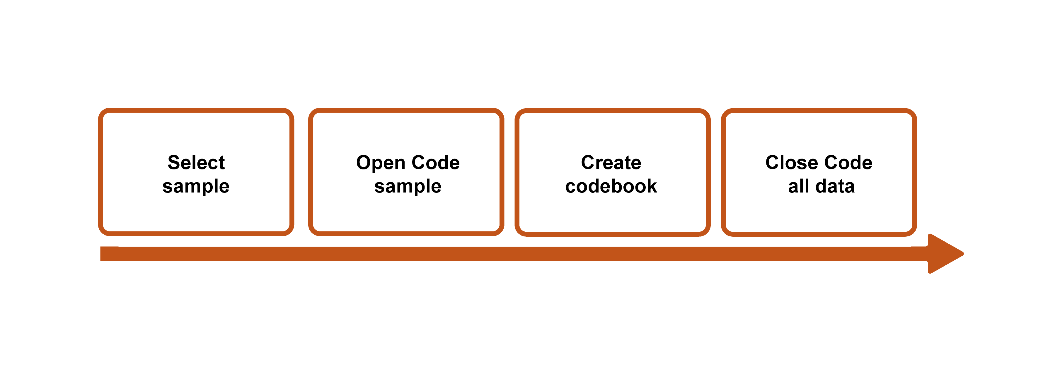
Second, code everything (“ open coding ”). See what emerges, and don’t limit yourself in any way. You will end up with a ton of codes, many more than you will end up with, but this is an excellent way to not foreclose an interesting finding too early in the analysis. Note the importance of starting with a sample of your collected data, because otherwise, open coding all your data is, frankly, impossible and counterproductive. You will just get stuck in the weeds.

Third, pare down your coding list. Where you may have begun with fifty (or more!) codes, you probably want no more than twenty remaining. Go back through the weeds and pull out everything that does not have the potential to bloom into a nicely shaped garden. Note that you should do this before tackling all of your data . Sometimes, however, you might need to rethink the sample you chose. Let’s say that the graduate student interview brought up some interesting gender issues that were pertinent to female-identifying sociologists, but both the junior and the senior faculty members identified as male. In that case, I might read through and open code at least one other interview transcript, perhaps a female-identifying senior faculty member, before paring down my list of codes.

This is also the time to create a codebook if you are using one, a master guide to the codes you are using, including examples (see Sample Codebooks 1 and 2 ). A codebook is simply a document that lists and describes the codes you are using. It is easy to forget what you meant the first time you penciled a coded notation next to a passage, so the codebook allows you to be clear and consistent with the use of your codes. There is not one correct way to create a codebook, but generally speaking, the codebook should include (1) the code (either name or identification number or both), (2) a description of what the code signifies and when and where it should be applied, and (3) an example of the code to help clarify (2). Listing all the codes down somewhere also allows you to organize and reorganize them, which can be part of the analytical process. It is possible that your twenty remaining codes can be neatly organized into five to seven master “themes.” Codebooks can and should develop as you recursively read through and code your collected material. [3]

Fourth, using the pared-down list of codes (or codebook), read through and code all the data. I know many qualitative researchers who work without a codebook, but it is still a good practice, especially for beginners. At the very least, read through your list of codes before you begin this “ closed coding ” step so that you can minimize the chance of missing a passage or section that needs to be coded. The final step is…to do it all again. Or, at least, do closed coding (step four) again. All of this takes a great deal of time, and you should plan accordingly.

Researcher Note

People often say that qualitative research takes a lot of time. Some say this because qualitative researchers often collect their own data. This part can be time consuming, but to me, it’s the analytical process that takes the most time. I usually read every transcript twice before starting to code, then it usually takes me six rounds of coding until I’m satisfied I’ve thoroughly coded everything. Even after the coding, it usually takes me a year to figure out how to put the analysis together into a coherent argument and to figure out what language to use. Just deciding what name to use for a particular group or idea can take months. Understanding this going in can be helpful so that you know to be patient with yourself.

—Jessi Streib, author of The Power of the Past and Privilege Lost 

Note that there is no magic in any of this, nor is there any single “right” way to code or any “correct” codes. What you see in the data will be prompted by your position as a researcher and your scholarly interests. Where the above codes on a preschooler solving a puzzle emerged from my own interest in puzzle solving, another researcher might focus on something wholly different. A scholar of linguistics, for example, may focus instead on the verbalizations made by the child during the discovery process, perhaps even noting particular vocalizations (incidence of grrrs and gritting of the teeth, for example). Your recording of the codes you used is the important part, as it allows other researchers to assess the reliability and validity of your analyses based on those codes. Chapter 19 will provide more details about the kinds of codes you might develop.

Saldaña ( 2014 ) lists seven “necessary personal attributes” for successful coding. To paraphrase, they are the following:

• Having (or practicing) good organizational skills
• Perseverance
• The ability and willingness to deal with ambiguity
• Flexibility
• Creativity, broadly understood, which includes “the ability to think visually, to think symbolically, to think in metaphors, and to think of as many ways as possible to approach a problem” (20)
• Commitment to being rigorously ethical
• Having an extensive vocabulary [4]

Writing Analytic Memos during/after Coding

Coding the data you have collected is only one aspect of analyzing it. Too many beginners have coded their data and then wondered what to do next. Coding is meant to help organize your data so that you can see it more clearly, but it is not itself an analysis. Thinking about the data, reviewing the coded data, and bringing in the previous literature (here is where you use your literature review and theory) to help make sense of what you have collected are all important aspects of data analysis. Analytic memos are notes you write to yourself about the data. They can be short (a single page or even a paragraph) or long (several pages). These memos can themselves be the subject of subsequent analytic memoing as part of the recursive process that is qualitative data analysis.

Short analytic memos are written about impressions you have about the data, what is emerging, and what might be of interest later on. You can write a short memo about a particular code, for example, and why this code seems important and where it might connect to previous literature. For example, I might write a paragraph about a “cultural capital” code that I use whenever a working-class sociologist says anything about “not fitting in” with their peers (e.g., not having the right accent or hairstyle or private school background). I could then write a little bit about Bourdieu, who originated the notion of cultural capital, and try to make some connections between his definition and how I am applying it here. I can also use the memo to raise questions or doubts I have about what I am seeing (e.g., Maybe the type of school belongs somewhere else? Is this really the right code?). Later on, I can incorporate some of this writing into the theory section of my final paper or article. Here are some types of things that might form the basis of a short memo: something you want to remember, something you noticed that was new or different, a reaction you had, a suspicion or hunch that you are developing, a pattern you are noticing, any inferences you are starting to draw. Rubin ( 2021 ) advises, “Always include some quotation or excerpt from your dataset…that set you off on this idea. It’s happened to me so many times—I’ll have a really strong reaction to a piece of data, write down some insight without the original quotation or context, and then [later] have no idea what I was talking about and have no way of recreating my insight because I can’t remember what piece of data made me think this way” ( 203 ).

All CAQDAS programs include spaces for writing, generating, and storing memos. You can link a memo to a particular transcript, for example. But you can just as easily keep a notebook at hand in which you write notes to yourself, if you prefer the more tactile approach. Drawing pictures that illustrate themes and patterns you are beginning to see also works. The point is to write early and write often, as these memos are the building blocks of your eventual final product (chapter 20).

In the next chapter (chapter 19), we will go a little deeper into codes and how to use them to identify patterns and themes in your data. This chapter has given you an idea of the process of data analysis, but there is much yet to learn about the elements of that process!

Qualitative Data-Analysis Samples

The following three passages are examples of how qualitative researchers describe their data-analysis practices. The first, by Harvey, is a useful example of how data analysis can shift the original research questions. The second example, by Thai, shows multiple stages of coding and how these stages build upward to conceptual themes and theorization. The third example, by Lamont, shows a masterful use of a variety of techniques to generate theory.

Example 1: “Look Someone in the Eye” by Peter Francis Harvey ( 2022 )

I entered the field intending to study gender socialization. However, through the iterative process of writing fieldnotes, rereading them, conducting further research, and writing extensive analytic memos, my focus shifted. Abductive analysis encourages the search for unexpected findings in light of existing literature. In my early data collection, fieldnotes, and memoing, classed comportment was unmistakably prominent in both schools. I was surprised by how pervasive this bodily socialization proved to be and further surprised by the discrepancies between the two schools.…I returned to the literature to compare my empirical findings.…To further clarify patterns within my data and to aid the search for disconfirming evidence, I constructed data matrices (Miles, Huberman, and Saldaña 2013). While rereading my fieldnotes, I used ATLAS.ti to code and recode key sections (Miles et al. 2013), punctuating this process with additional analytic memos. ( 2022:1420 )

Example 2:” Policing and Symbolic Control” by Mai Thai ( 2022 )

Conventional to qualitative research, my analyses iterated between theory development and testing. Analytical memos were written throughout the data collection, and my analyses using MAXQDA software helped me develop, confirm, and challenge specific themes.…My early coding scheme which included descriptive codes (e.g., uniform inspection, college trips) and verbatim codes of the common terms used by field site participants (e.g., “never quit,” “ghetto”) led me to conceptualize valorization. Later analyses developed into thematic codes (e.g., good citizens, criminality) and process codes (e.g., valorization, criminalization), which helped refine my arguments. ( 2022:1191–1192 )

Example 3: The Dignity of Working Men by Michèle Lamont ( 2000 )

To analyze the interviews, I summarized them in a 13-page document including socio-demographic information as well as information on the boundary work of the interviewees. To facilitate comparisons, I noted some of the respondents’ answers on grids and summarized these on matrix displays using techniques suggested by Miles and Huberman for standardizing and processing qualitative data. Interviews were also analyzed one by one, with a focus on the criteria that each respondent mobilized for the evaluation of status. Moreover, I located each interviewee on several five-point scales pertaining to the most significant dimensions they used to evaluate status. I also compared individual interviewees with respondents who were similar to and different from them, both within and across samples. Finally, I classified all the transcripts thematically to perform a systematic analysis of all the important themes that appear in the interviews, approaching the latter as data against which theoretical questions can be explored. ( 2000:256–257 )

Sample Codebook 1

This is an abridged version of the codebook used to analyze qualitative responses to a question about how class affects careers in sociology. Note the use of numbers to organize the flow, supplemented by highlighting techniques (e.g., bolding) and subcoding numbers.

01. CAPS: Any reference to “capitals” in the response, even if the specific words are not used

01.1: cultural capital 01.2: social capital 01.3: economic capital

(can be mixed: “0.12”= both cultural and asocial capital; “0.23”= both social and economic)

01. CAPS: a reference to “capitals” in which the specific words are used [ bold : thus, 01.23 means that both social capital and economic capital were mentioned specifically

02. DEBT: discussion of debt

02.1: mentions personal issues around debt 02.2: discusses debt but in the abstract only (e.g., “people with debt have to worry”)

03. FirstP: how the response is positioned

03.1: neutral or abstract response 03.2: discusses self (“I”) 03.3: discusses others (“they”)

Sample Coded Passage:

* Question: What other codes jump out to you here? Shouldn’t there be a code for feelings of loneliness or alienation? What about an emotions code ?

Sample Codebook 2

This is an example that uses "word" categories only, with descriptions and examples for each code

Further Readings

Elliott, Victoria. 2018. “Thinking about the Coding Process in Qualitative Analysis.” Qualitative Report 23(11):2850–2861. Address common questions those new to coding ask, including the use of “counting” and how to shore up reliability.

Friese, Susanne. 2019. Qualitative Data Analysis with ATLAS.ti. 3rd ed. A good guide to ATLAS.ti, arguably the most used CAQDAS program. Organized around a series of “skills training” to get you up to speed.

Jackson, Kristi, and Pat Bazeley. 2019. Qualitative Data Analysis with NVIVO . 3rd ed. Thousand Oaks, CA: SAGE. If you want to use the CAQDAS program NVivo, this is a good affordable guide to doing so. Includes copious examples, figures, and graphic displays.

LeCompte, Margaret D. 2000. “Analyzing Qualitative Data.” Theory into Practice 39(3):146–154. A very practical and readable guide to the entire coding process, with particular applicability to educational program evaluation/policy analysis.

Miles, Matthew B., and A. Michael Huberman. 1994. Qualitative Data Analysis: An Expanded Sourcebook . 2nd ed. Thousand Oaks, CA: SAGE. A classic reference on coding. May now be superseded by Miles, Huberman, and Saldaña (2019).

Miles, Matthew B., A. Michael Huberman, and Johnny Saldaña. 2019. Qualitative Data Analysis: A Methods Sourcebook . 4th ed. Thousand Oaks, CA; SAGE. A practical methods sourcebook for all qualitative researchers at all levels using visual displays and examples. Highly recommended.

Saldaña, Johnny. 2014. The Coding Manual for Qualitative Researchers . 2nd ed. Thousand Oaks, CA: SAGE. The most complete and comprehensive compendium of coding techniques out there. Essential reference.

Silver, Christina. 2014. Using Software in Qualitative Research: A Step-by-Step Guide. 2nd ed. Thousand Oaks, CA; SAGE. If you are unsure which CAQDAS program you are interested in using or want to compare the features and usages of each, this guidebook is quite helpful.

Vogt, W. Paul, Elaine R. Vogt, Diane C. Gardner, and Lynne M. Haeffele2014. Selecting the Right Analyses for Your Data: Quantitative, Qualitative, and Mixed Methods . New York: The Guilford Press. User-friendly reference guide to all forms of analysis; may be particularly helpful for those engaged in mixed-methods research.

• When you have collected content (historical, media, archival) that interests you because of its communicative aspect, content analysis (chapter 17) is appropriate. Whereas content analysis is both a research method and a tool of analysis, coding is a tool of analysis that can be used for all kinds of data to address any number of questions. Content analysis itself includes coding. ↵
• Scientific research, whether quantitative or qualitative, demands we keep an open mind as we conduct our research, that we are “neutral” regarding what is actually there to find. Students who are trained in non-research-based disciplines such as the arts or philosophy or who are (admirably) focused on pursuing social justice can too easily fall into the trap of thinking their job is to “demonstrate” something through the data. That is not the job of a researcher. The job of a researcher is to present (and interpret) findings—things “out there” (even if inside other people’s hearts and minds). One helpful suggestion: when formulating your research question, if you already know the answer (or think you do), scrap that research. Ask a question to which you do not yet know the answer. ↵
• Codebooks are particularly useful for collaborative research so that codes are applied and interpreted similarly. If you are working with a team of researchers, you will want to take extra care that your codebooks remain in synch and that any refinements or developments are shared with fellow coders. You will also want to conduct an “intercoder reliability” check, testing whether the codes you have developed are clearly identifiable so that multiple coders are using them similarly. Messy, unclear codes that can be interpreted differently by different coders will make it much more difficult to identify patterns across the data. ↵
• Note that this is important for creating/denoting new codes. The vocabulary does not need to be in English or any particular language. You can use whatever words or phrases capture what it is you are seeing in the data. ↵

A first-cycle coding process in which gerunds are used to identify conceptual actions, often for the purpose of tracing change and development over time.  Widely used in the Grounded Theory approach.

A first-cycle coding process in which terms or phrases used by the participants become the code applied to a particular passage.  It is also known as “verbatim coding,” “indigenous coding,” “natural coding,” “emic coding,” and “inductive coding,” depending on the tradition of inquiry of the researcher.  It is common in Grounded Theory approaches and has even given its name to one of the primary CAQDAS programs (“NVivo”).

Computer-assisted qualitative data-analysis software.  These are software packages that can serve as a repository for qualitative data and that enable coding, memoing, and other tools of data analysis.  See chapter 17 for particular recommendations.

The purposeful selection of some data to prove a preexisting expectation or desired point of the researcher where other data exists that would contradict the interpretation offered.  Note that it is not cherry picking to select a quote that typifies the main finding of a study, although it would be cherry picking to select a quote that is atypical of a body of interviews and then present it as if it is typical.

A preliminary stage of coding in which the researcher notes particular aspects of interest in the data set and begins creating codes.  Later stages of coding refine these preliminary codes.  Note: in Grounded Theory , open coding has a more specific meaning and is often called initial coding : data are broken down into substantive codes in a line-by-line manner, and incidents are compared with one another for similarities and differences until the core category is found.  See also closed coding .

A set of codes, definitions, and examples used as a guide to help analyze interview data.  Codebooks are particularly helpful and necessary when research analysis is shared among members of a research team, as codebooks allow for standardization of shared meanings and code attributions.

The final stages of coding after the refinement of codes has created a complete list or codebook in which all the data is coded using this refined list or codebook.  Compare to open coding .

A first-cycle coding process in which emotions and emotionally salient passages are tagged.

Introduction to Qualitative Research Methods Copyright © 2023 by Allison Hurst is licensed under a Creative Commons Attribution-ShareAlike 4.0 International License , except where otherwise noted.

Quantitative Data Presentation and Analysis: Descriptive Analysis

• First Online: 01 October 2022

Cite this chapter

• Charitha Harshani Perera 4 ,
• Rajkishore Nayak 5 &
• Long Van Thang Nguyen 6  

470 Accesses

This chapter provides a descriptive analysis of the quantitative data and is divided into five sections. The first section presents the preliminary consideration of data, showing the response rate and the process of data screening and cleaning.

Download chapter PDF

5.1 Introduction

This chapter provides a descriptive analysis of the quantitative data and is divided into five sections. The first section presents the preliminary consideration of data, showing the response rate and the process of data screening and cleaning. The second section deals with the demographic profiles of the respondents. The third section provides a preliminary reliability assessment of the primary constructs in the present study. The fourth section deals with findings from the descriptive analysis of the data obtained on the study’s major observed constructs, and finally, the fifth section offers a summary.

5.2 Preliminary Data Consideration

5.2.1 response rate.

The researcher personally administered the questionnaire. A survey was conducted on weekdays between 10.00 a.m. and 5.00 p.m. This ensures that students from different studying years and fields were primed to respond as lecture times vary depending on the availability of the lecture halls and the lecturers. During pilot testing, it was determined that students were more receptive after lecture time to complete the survey instrument than at the starting time. No compensation was provided to students for completing or attempting to complete the survey. The researcher spent two months collecting data, one month in each country. The researcher personally visited each HEI for the survey with the permission of their administration. After a brief explanation of the survey’s purpose, the questionnaires were distributed based on the students’ willingness to participate.

Though the sample size is 800 (400 from each country), 1150 questionnaires were distributed, anticipating issues in collecting and analysing data. Of 500 distributed questionnaires in Sri Lanka and 650 in Vietnam, 412 (Sri Lanka) and 581 (Vietnam) were considered to be valid for subsequent quantitative analysis. Table 5.1 details the response rate, which represents the full research sample. A total of 1040 questionnaires were returned from both countries, but 47 of them were unusable for the following reasons: respondents had circled many responses for one question Likert scale items (36 cases) and many missing responses (11 cases). When incomplete and unusable responses were removed, a total of 993 valid responses were available for further analysis. All items of the questionnaire were coded before feeding data into the analysis software and carefully reviewed to identify incomplete or extreme cases. Accordingly, 993 questionnaires were considered valid for further data analysis, thereby giving a high response rate of 86.3% of the original sample size. It is worth mentioning that such a high response rate might be the outcome of the purposive sampling technique, which provided the researcher with the guarantee that the findings could be interesting to generalise.

The next step was to screen and clean the collected raw data to ensure the accuracy of the statistical techniques used in the study.

Bias is a type of error that systematically skews results in a certain direction. Selection bias is a kind of error that occurs when the researcher decides who is going to be studied. It is usually associated with research where the selection of participants isn’t random (i.e., with observational studies such as cohort, case–control, and cross-sectional studies). Selection bias also occurs when people volunteer for a study. Those who choose to join (i.e., who self-select into the study) may share a characteristic that makes them different from non-participants from the get-go.

In order to overcome self-selection bias first, the researcher makes their study representative by including as many people as possible. Then the researcher has conducted an experimental study in which participants are randomly assigned to the present study. In designing the experimental study, the researcher has focused on the social media usage of the undergraduates, and their engagement with their respective HEIs’ social networking sites. The evaluations attempt to avoid selection bias by making the control group as comparable as possible, typically by matching on observables. The more data that is available for matching, the more convincing this is. The minimum number of respondents for the study is 800 and 400 from each country. In order to gain the required number of participants, the researcher distributed 500–600 questionnaires, and screening questions were included to match the subgroups with the population. Since, this study selects two samples from two countries, by including screening questions, this study minimised the bias and ensured that the selected sample represents the total population.

5.2.2 Data Screening and Cleaning

According to Hair et al. ( 2014 ), different multivariate statistical techniques, including factor analysis and SEM, have the tremendous theoretical ability to help researchers in various fields to test their hypotheses and assess the viability of their proposed models. However, such techniques are not without restrictions. Therefore, data screening and cleaning are considered a significant concern when the intention is to use multivariate analysis. It might be time-consuming and exhaustive, as noted by Kline ( 2011 ).

In data screening and cleaning, the researcher followed the methods below to check the appropriateness of numerical values of each variable under study. Table 5.2 summarises all the data screening and cleaning methods adopted in this study.

The preliminary data screening was performed by checking the basic frequency and descriptive statistics distributions. Any odd or wrongly coded values were detected and then properly corrected. However, several cases were found to have missing responses. Table 5.3 shows the frequencies and the percentages of missing data.

Scheffer ( 2002 ) claims that regardless of how much a researcher attempts to have a full dataset in response to any particular survey or how well s/he has designed an experiment, missing data afflict almost all research efforts. Hair et al. ( 2014 ) highlight that the problem of missing data affects the statistical analysis of the original dataset in two ways; firstly, by reducing the power of the statistical techniques in indicating any relationships in the dataset; and secondly, by generating bias in the process of parameter estimations.

Although no clear rule about the acceptable percentage of missing data appears in the literature, researchers suggest that less than 1% of missing values of any variable is usually considered very slight and unimportant, 1–5% remains manageable by many statistical methods, 5–15% requires more unconventional and complicated techniques to deal with, and more than 15% missing values of a given dataset could harshly distort any kind of further data interpretation (Acuna & Rodriguez, 2004 ; Cohen et al., 2013 ). Additionally, Hair et al. ( 2014 ) and Kline ( 2011 ) claim that when the amount of missing values within a large dataset is relatively small, the researcher faces a less serious problem and could treat those missing values quickly since any treatment option could lead to similar results.

Table 5.3 shows that the maximum percentage of missing data for the questionnaire items in the current study was 0.3%, meaning that this is extremely low and within a satisfactory level. Hence, the researcher faces a less severe problem and could treat those missing values effortlessly since any treatment option could lead to similar results.

As mistakes of data entries are the possible consequences of missing values, the researcher double-checked all entries to minimise feeding wrong data into the analysis programme. However, to treat those missing values, the researcher decided to apply regression-based imputation as this method takes into consideration the relationships among different variables based on the overall responses, thereby leading to more accurate value estimation (Kline, 2011 ). Regression-based imputation is the best method to generate the predicted score for a missing value since other methods are mainly on pattern matching, which does not guarantee to have the most similar pattern of scores (Kline, 2011 ).

After treating the missing values, the next logical step was to consider outliers (univariate and multivariate), representing those cases with odd and/or extreme scores from other dataset observations. Errors in data entry, erroneous sampling techniques, missing values in the calculation, and extreme responses on multi-point scales are among the many causes of outliers.

First, a check for univariate outliers was applied. On each of the variable observations, univariate outliers were identified by using z-score frequency distributions. All scores for each variable were converted to standard scores (z-scores) and then checked against the intended range. As a rule of thumb, a range of (±3 to ± 4) z-scores for samples larger than 80 was considered acceptable, with any individual observation exceeding that limits being treated as a univariate outlier (Hair et al., 2014 ). The z-scores of ± 3.29—the z-score that corresponds to a probability of 0.001—were used to identify any odd values within each variable’s observations. No standard score less than −3.29 or greater than +3.29 was identified from all research variables, which means the absence of univariate outliers from the dataset of the current study (Table 5.4 ).

Next, multivariate outliers were detected by calculating the Mahalanobis distance ( D 2 ), which represents the distance of a case from the multidimensional mean of a distribution. Mahalanobis D 2 with a probability less than or equal to 0.001, eliminated those cases from the datasheet to maintain more representative samples. However, the data set did not detect any Mahalanobis D 2 with p ˂ 0.001. Thus, requiring further consideration on outliers did not want for the current data set.

The normality of the data distribution is considered as one of the most critical assumptions underlying various multivariate analysis tools such as factor analysis and SEM. The multivariate normality of a particular distribution confirms that the shape of individual variables’ distribution or the distribution of a combination of two or more variables is corresponding with the bell-shaped normal distribution (Doornik & Hansen, 2008 ; Hair et al., 2014 ). Any violation of the normality assumption could severely affect the process of data analysis and goodness-of-fit indices for the proposed SEM model (Andrews et al., 1973 ; Kline, 2011 ; Korkmaz et al., 2014 ).

Skewness and Kurtosis are two ways of considering data that indicate the normality of a given dataset distribution (Doornik & Hansen, 2008 ; Thulin, 2014 ). Skewness demonstrates the symmetry of distribution, while Kurtosis refers to how much the distribution is peaked or flat compared with the normal distribution (Hair et al., 2010; Andrews et al., 2014 ). In general, a normally distributed distribution has skewness and kurtosis values of zero. However, scholars provide general guidelines about when skewness and kurtosis values might become problematic. For example, Hair et al. (2010) suggested that any skewness and kurtosis values falling outside the range of −1 to +1 represent a potential normality problem.

Conversely, many researchers are less conservative, recommending that skewness less than an absolute value of 3 and a kurtosis index with an absolute value of less than 8 does not indicate a significant normality problem (Doornik & Hansen, 2008 ; Kline, 2011 ; West et al., 1995 ).

In the current study, all individual measured items were tested for normality using skewness and kurtosis statistics as shown in Table 5.5 , which reveals that for the 34 items, the skewness was in the range of −0.339 to 0.250, and kurtosis was in the range of −0.701 to 0.201. This indicates no significant deviation from the normal distribution.

A further normality assessment was made from the residual analysis using the expected normality P-P plot for the regression residuals, shown in Fig.  5.1 . An acceptable normality level was revealed as the standardised predicted value formed a line with the standardised residuals. P-P plots for each variable were separately depicted in Appendix 5A.

Normal P-P plot of regression standardised residual

5.3 Background and Demographic Profile of the Study Sample

The results relating to parts one and two of the questionnaire, i.e., demographic data and social media and traditional media users, are now presented and described. Frequency distributions with respect to demographics and social media usage clarify the study sample characteristics.

5.3.1 Demographics

Table 5.6 summarises the demographic data relating to gender, year, the field of study, hours on social media, widely used social networking site, how often on the most preferred social networking site, level of involvement with posting and commenting on social media posts, and hours on traditional media.

It reveals that the gender breakdown was 31.10% male and 68.90% female. The sample consists of more female customers than male. This is justified when compared with the general gender distribution of Sri Lanka and Vietnam. The results agree with the latest reported gender profile in Sri Lanka and Vietnam, which is 48.4% and 51.6% for males and females, respectively, in Sri Lanka (Census and Statistics Department, 2017), and 49.3% and 50.7 for males and females, respectively, in Vietnam (OECD, 2017 ).

Concerning the studying year, responses were received from the undergraduates from different study years starting from 1st year to 4th year; 41.0%, 12.2%, 31.4%, and 15.4% of undergraduates are studying in 1st year, 2nd year, 3rd year, and 4th year, respectively. Most undergraduates were in the 1st Year (41.0%), while other years represented a lower level of undergraduate population.

The respondents were clustered into five groups as per the field of study to represent all the study streams in any HEI. According to the sample profile, 5.2% of the undergraduates are majoring in Information technology. Those studying Business Administration, Financial & accounting, and Marketing accounted for 14.8%, 34.9%, and 3.5%, respectively, while 41.5% of the undergraduates represented the other field of studies such as agriculture, tourism and hospitality management, quantity surveying, etc.

The average time on social media was identified based on the active participation hours with social media. It shows a higher percentage in the last category, representing social media usage for more than 4 h (41.8%). The lowest number of respondents use social media for less than one hour (3.7%). The average social media usage per day indicates through 2–3 h. According to Vietnam Digital Landscape (2018), the average daily time spent using social media in Vietnam was 2 h and 37 min.

As the researcher expected, the most widely used social networking site among the selected sample was Facebook; 49.3% of Facebook users indicate that nearly half of the sample respondents use Facebook more than other social networking sites. According to Vietnam’s Digital Landscape ( 2019 ) and Digital Sri Lanka (2018), the widely used SNS in both countries was Facebook, and the second position was owned by YouTube (15.1%). To some extent, this is consistent with the study results. However, other social networking sites indicated a lower level of usage, i.e., Instagram (14.0%), Pinterest (12.0%), Google+ (8.5%), and other social networking sites such as Twitter (1.1%).

The average time on the preferred SNS was identified based on five categories. It shows that the majority of the participants visit their preferred SNS at least once per day (86.4%). Similarly, a negligible number of participants (0.9%) visit SNS less than once per month, while 10.2% of the social media users share information at least one time a week, denoting a higher level of a tendency towards social media activities.

Most respondents spend less than one hour on traditional media; 64.7% of respondents use traditional media for less than one hour, while 8.0% use more than 3 h. On average, Vietnamese use social media 7 h per day and traditional media 3 h per day, indicating a higher tendency towards social media than traditional media such as newspapers, television, and radio (Global web index, 2017).

5.4 Respondents’ Segmentation

The sample was divided into two groups, Sri Lanka and Vietnam, to clarify social media adoption. Various associations between the two groups were then performed to discover whether respondents differed based on their demographic characteristics.

5.4.1 Sri Lankans and Vietnamese Demographic Observations on Dependence

Observations of Sri Lankan and Vietnamese undergraduates in terms of the demographic characteristics of gender, studying year, the field of study, hours on social media, widely used SNSs, how often they visit the SNSs, how often they post information or comments in SNSs, and hours on social media are now presented. Chi-square tests were performed to examine the impact of these demographic variables on the two groups’ decisions to adopt social media in Sri Lanka and Vietnam. At this point, it is essential to have a good understanding of the Chi-square test and its underlying assumptions.

The Chi-square test for independence is a non-parametric technique that explores any significant relationship between two categorical variables from the same sample. This test begins with the hypothesis of no association or no relationship between the two variables under consideration (the null hypothesis). The alternate hypothesis states that the two variables are associated. The decision to reject or accept the null hypothesis depends on the p-value associated with the Chi-square statistic. If the p-value is less than a predetermined significance level (usually 0.05), the null hypothesis is rejected, then the assumption that the two variables are independent (no association) is rejected, and the alternate hypothesis assumption of the association between the two variables is accepted.

Like any other statistical technique, the Chi-square test makes some specific assumptions about the data to ensure the statistical suitability of the test. The first assumption relates to the sampling method, which must involve a random sample chosen from the entire population. The second assumption is that the sample is large enough, with the population for each variable being at least ten times larger than the sample. The third assumption is that the two variables are both categorical. The last assumption is that the expected frequency of any sub-category of the two variables is at least five. More specifically, in any frequency table, each frequency cell of the table should present five or more expected frequency counts (Field, 2009 ; Pallant, 2013 ).

A preliminary check of the data was conducted to ensure no violation of any of the above assumptions. This revealed that all assumptions were met for all involved variables except the last one (expected frequencies assumption) for two sub-categories in two variables: those who are using “other” social networking sites, and those who visit social networking sites “Less than one time a month”. The expected frequencies in those were 4.6 and 3.7. Therefore, the two sub-categories above were excluded when applying the test to keep all Chi-square test assumptions unviolated.

5.4.1.1 Gender Observations

The gender distribution of the respondents was as follows: 412 respondents were Sri Lankans (41.5% of the total respondents) of which, 150 were males (36.4% of the total Sri Lankans), and 262 were females (63.6% of the total Sri Lankans). Of 581 Vietnamese respondents (58.5% of the total respondents), 159 respondents were males (27.3% of the total Vietnamese), and 422 were females (72.7% of the total).

The null hypothesis was rejected since the p -value (0.002) is less than the significance level (0.05). The Chi-square statistics (χ 2 (1) = 9.193) in Appendix 5C revealed a significant association between the respondent’s gender and location. This association reflects that among male respondents, about 48.5% were Sri Lankans and 51.5% were Vietnamese; in females, about 61.7% were Vietnamese, and only 38.3% of them were Sri Lankans, as shown in Appendix 5C.

This study selected respondents mainly based on social media usage. As per the above results, it can be concluded that the gender of the respondents had a significant influence since males in Sri Lanka and females in Vietnam are more willing to use social media than their counterparts. So that in implementing social media marketing strategies for branding in Sri Lanka and Vietnam, firms need to focus on the target niche based on their gender.

5.4.1.2 Studying Year Observations

The studying year of Sri Lankans and Vietnamese shown in Appendix 5D reveals that most Sri Lankans were 1st year and 3rd year students (75.9% of the total Sri Lankans). Further, while almost 10.9% of the total number of Sri Lankans were 2nd year students, 35.2% of them were 4th year students. Appendix 5D indicates that most Vietnamese were also in the 1 st and 3 rd years, with 42.7% and 27.2%, respectively.

This is obvious in the gaps between the percentages of Sri Lankan and Vietnamese social media users within their studying years. Therefore, in implementing branding strategies on social media, both Sri Lankans and Vietnamese should focus more on the 1st and 3rd year students than the ones in the 2nd and 4th years.

5.4.1.3 Field of Study Observations

In terms of field of study, Appendix 5E shows that social media users in Sri Lanka came mainly from Finance & Accounting, which accounted for 40.5%. Participants who study IT represented 5.3%, business administration represented 17.8%, marketing represented 2.4%, and the remaining 34.0% were from other subject areas such as agriculture, quantity surveying, etc.

Appendix 5E also shows that the majority of the undergraduates in Vietnam from other fields (agriculture, hospitality, quantity survey, etc.) accounted for 46.8%. The Chi-square results as depicted in Appendix 5 K indicated that studying year and the location are associated (χ 2 (4) = 22.329, p  < 0.05), denoting that students in Finance & Accounting and other fields tend to be more willing to use the social media.

5.4.1.4 Hours of Social Media Observations

The hours spent on social media by participants, as illustrated in Appendix 5F, show that two categories dominated Sri Lankans and Vietnamese. Most Sri Lankans were using social media between 3–4 h or more than 4 h (63.8%), and the majority of Vietnamese were also from these two categories (65.4%).

The frequency distributions of Sri Lankans and Vietnamese within the same hours on social media (Appendix 5F) show that 36.2% and 34.6% of the respondents from Sri Lanka and Vietnam, respectively, use social media for less than 3 h. Appendix 5K shows a slight similarity in social media usage among the Sri Lankans and Vietnamese. Therefore, it could be concluded that the hours on social media in Sri Lankans and Vietnamese do not account for a significant variation.

Chi-square results (χ 2 (4) = 0.851, p  > 0.05) provide more support for this finding since they indicated no significant association between the hours on social media and Sri Lankans and Vietnamese’ decisions to use social media.

5.4.1.5 Widely Used Social Networking Sites Observations

Social networking sites (SNSs), a subdomain of social media, have been defined as a network communication platform in which participants (1) have uniquely identifiable profiles that consist of user-supplied content, content provided by other users, and/or system-provided data; (2) can publicly articulate connections that can be viewed and traversed by others; and (3) can consume, produce, and/or interact with streams of user-generated content provided by their connections on the site (Ellison & Boyd, 2013 , p. 157).

Appendix 5G lists the widely used social networking sites of Sri Lankans and Vietnamese. The majority of Sri Lankans use Facebook and Instagram, accounting for 26.9% and 25.2%, respectively, whereas 47.8% of total Sri Lankans used other social networking sites such as YouTube, Pinterest, and Google+. Similarly, 72.0% and 15.0% of Vietnamese were using Facebook and YouTube, respectively, reflecting the majority.

Based on the above discussion, it can be concluded that an association exists between widely used social networking sites and social media usage among Sri Lankans and Vietnamese. Additionally, the Chi-square results featured in Appendix 5K (χ 2 (5) = 383.968, p  < 0.05) confirm a significant association between the widely used social networking site and location. However, the results showed that social media users in both countries make their presence mainly on Facebook. Apart from that, Sri Lankans are increasingly using Instagram in connecting with people. In contrast, Vietnamese are more enthusiastic about using YouTube, as it provides everything descriptively. Hence, marketing managers of higher education institutes in Sri Lanka and Vietnam should focus on Instagram and YouTube, respectively, in implementing their branding strategies in addition to Facebook.

5.4.1.6 Frequency of Social Media Observations

How often the respondents visit their preferred social media sites, illustrated in Appendix 5H, shows that two categories dominated both Sri Lankans and Vietnamese. Most Sri Lankans visit social networking sites at least one time per week (12.8%) and at least one time per day (81.6%). Likewise, the majority of Vietnamese also use these two categories (98.1%).

How often Sri Lankans and Vietnamese visit social networking sites, at least one time per month or less, is accounted for 5.58% and 1.89% of Sri Lanka and Vietnam, respectively. Appendix 5H shows a slight similarity in the social media usage among the Sri Lankans and Vietnamese.

Chi-square results (χ 2 (4) = 21.850, p  > 0.05) provide more support for this finding since they indicated no significant variation between the frequency of visiting social networking sites and Sri Lankans and Vietnamese’ decision to use social media.

5.4.1.7 Frequency of Posting on Social Media Observations

The frequency of posting information and comments on social networking sites illustrated in Appendix 5I shows that two categories dominate the Sri Lankans. The majority of Sri Lankans were posting information and comments at least one time per week and at least one time per day, 83.0% indicating higher engagement with social networking sites.

In contrast, most Vietnamese post on social networking sites at least one time per month (21.3%) and only once in a few months (33.6). Later, the Chi-square results as depicted in Appendix 5 K indicated that how often the respondents post information or comment on social media and location are associated (χ 2 (4) = 328.590, p  < 0.05), signifying that more Sri Lankans tend to be willing to share information on social networking sites.

5.4.1.8 Traditional Media Usage Observations

The traditional media usage among the participants illustrated in Appendix 5J shows that two categories dominate both Sri Lankans and Vietnamese. Most Sri Lankans use traditional media for less than 1 h and between 1 and 3 h (89.6%), and the majority of Vietnamese were also from these two categories (93.8%).

The traditional media usage of Sri Lankans and Vietnamese for over 3 h shows that 10.4% and 6.2% of the respondents from Sri Lanka and Vietnam, respectively, use social media for less than 3 h.

Overall, the number of female undergraduate students worldwide has exceeded the number of men since 2002 (Co-operation & Development, 2021 ). Data from UNESCO’s Institute of Statistics(UIS) shows that between 2000 and 2018, the Gross Enrolment Ratio (GER) in tertiary enrolment for males increased from 19 to 36%, while that for females went from 19 to 41% (UNESCO-IESALC, 2021 ). Women have, therefore, been the main beneficiaries of the rapid increases in higher education enrolment making up the majority of undergraduate students in all regions (Vaughn et al., 2020 ). Not only do females make up most of the undergraduate students, but they are also more likely to complete higher education than their male counterparts (Berg, 2019 ).

The gender gap in higher education has virtually disappeared in most places (Barone & Assirelli, 2020 ). Women even outnumber men in higher education in many countries around the world, including developing countries across all regions (Neubauer, 2019 ). In Asia, especially, women’s enrolment has accelerated in recent years as the overall demand for higher education has accelerated (Cuthbert et al., 2019 ). A huge trend in higher education in Asia is increasing privatisation, which in many cases also created many educational opportunities available for women to study at private HEIs (Sanger & Gleason, 2020 ). Private HEIs have expanded women’s options by expanding the overall educational system in developing countries (Sanger & Gleason, 2020 ). In addition, the women’s experiences at HEIs are vastly different from those of men in terms of structure, nature, and facilities of HEIs which motivated the women to enrol at private HEIs rather than public HEIs (Neubauer, 2019 ). Accordingly, Sri Lanka and Vietnam also showed similar kinds of findings. In the Sri Lankan context, 36.4% of males and 63.6% of females are pursuing their higher studies in private HEIs. Similarly, in Vietnam, 27.3% of males, and 72.7% of females are studying at private HEIs. These findings further verify the findings of the previous studies indicating that females have more positive perceptions of private HEIs than males when doing their selection process.

Further, according to the findings, most of the students in Sri Lanka and Vietnam are pursuing their studies in the field of finance and accounting. 40.5% of Sri Lankans and 31.0% of Vietnamese are following fiance, and accounting courses indicate the majority. Lai et al. ( 2009 ) and Reus ( 2020 ) highlighted that numerous academic studies investigated ways to improve the design, structure, and delivery of finance courses at the undergraduate level. Some researchers focused on identifying the most important topics that can be covered in one course, and they identified that finance and accounting are the most important courses for the students who have enrolled in business management degree programmes (Alshehri, 2017 ; Lusardi, 2019 ). Accordingly, Mudzingiri et al. ( 2018 ) identified that, in recent years, many undergraduates are enrolling in finance-related subjects more than other business-related subjects due to their interest to learn about financial behaviour, risk preferences, and financial literacy. The finding also provides compelling evidence for the previous researches as the students’ enrolment rate for finance and accounting is significantly higher than the other courses. These findings highlighted that the students in developing countries are keener in understanding financial literacy, hence the majority follow the financing and accounting courses.

5.5 Descriptive Analysis of Respondents’ Responses

This section presents a descriptive analysis of the data obtained from the sample. The full results appear in Appendix 5B. The following sub-sections report responses from the sample on the major constructs of the present study in central tendency and dispersion.

The questionnaire consists of 5 major constructs measured by 34 different items (statements) using a seven-point Likert scale ranging from “strongly disagree” to “strongly agree”. Respondents were asked about their agreement or disagreement with each statement. Responses were coded as follows: number 1 indicated they “strongly disagreed” with the statement, number 2 “Disagree”, number 3 “somewhat disagree”, number 4 “neither disagree nor agree”, number 5 “somewhat agree”, number 6 “agree”, and number 7 “strongly agree”. Further, number 4 was chosen as the midpoint on the scale to make a distinction between the respondent’s agreement and disagreement.

Therefore, the average values of each construct were considered when estimating descriptive statistics. Accordingly, the mean and standard deviation of the five main constructs of the research model is given in Table 5.7 .

5.5.1 Firm-Generated Content

Respondents were asked to indicate the extent to which the undergraduates are satisfied with how the HEIs use social networking sites to provide information about the HEIs. The results show that the mean scores of the four items used to measure FGC are between 4.48 and 4.77, with a standard deviation ranging from 1.381 to 1494. It could be concluded that most respondents (the mean score is more than the midpoint of 4) have agreed about the FGC of HEIs in terms of providing HEI-related updated information while sharing and motivating them to follow HEIs’ official social networking sites and enhancing their overall attachment with the HEIs.

5.5.2 User-Generated Content

The findings reveal that the mean scores for UGC were between 4.05 and 4.19, indicating that a significant number of respondents find HEIs’ information on other social networking sites interesting and useful. They consider the information shared by others helps them gather required information on HEIs while attractively providing the information. Moreover, the descriptive statistics for UGC also revealed that the respondents were not very dispersed around their mean scores on individual items (standard deviations between 1.458 and 1.600).

5.5.3 Brand Credibility

Regarding the brand credibility construct, respondents were asked to respond to five statements to measure the level of trust the undergraduates have towards their HEIs. The mean scores reveal an average of 4.3573, indicating that a relatively high level of agreement existed among respondents about this construct. To put it differently, undergraduates believe the HEIs can perform what they promise, the endowed HEIs’ quality is trustworthy, and HEI does not try to create a false image for society. Besides, the average standard deviation of 1.12291 indicates a little dispersion from that mean score.

5.5.4 Customer-Based Brand Equity

Respondents were asked to provide their opinions concerning seventeen statements related to the degree to which they perceived the service outcomes of HEIs as satisfying the students’ requirements. The findings revealed that the three items had means over three (i.e., midpoint) and an average mean of 4.5671, indicating that a relatively high level of agreement existed among respondents about this construction. Respondents had a good feeling about their HEI in creating value for HEI. Again, the average standard deviation was 0.98045, indicating low dispersion among respondents’ scores around the average mean.

5.5.5 Subjective Norm

Four items were used to measure the SN construct in this study. The mean scores were 4.31, 4.35, 4.19, and 4.45, all above the midpoint of four on the seven-point Likert scale. The average mean score was 4.3280, which indicated the participants’ agreement on the scale measures. Specifically, these results mean that most respondents accepted and were influenced by the information shared by social networks or acquaintances in choosing an HEI to pursue higher studies. The average standard deviation was 1.23502, indicating low dispersion among respondents’ scores around the average mean.

5.6 Summary

This chapter shows that the response rate to the questionnaire was sound at 90.4%, this being accounted for by 993 usable questionnaires for statistical analysis from the original 1150 distributed among both Sri Lankans and Vietnamese. Analysis of the respondents’ demographic profile by combining information gathered from both countries reveals several similarities between the study sample and the general population structure of Sri Lanka and Vietnam. The following chapter continues the quantitative data analysis by discussing the findings of factor analysis and SEM.

Acuna, E., & Rodriguez, C. (2004). The treatment of missing values and its effect on classifier accuracy. Classification, clustering, and data mining applications. Springer.

Google Scholar  

Alshehri, A. F. (2017). Student satisfaction and commitment towards a blended learning finance course: A new evidence from using the investment model. Research in International Business and Finance, 41 , 423–433.

Article   Google Scholar  

Andrews, D., Gnanadesikan, R., & Warner, J. (1973). Methods for assessing multivariate normality . Elsevier.

Book   Google Scholar  

Andrews, D., Gnanadesikan, R., Warner, J., & Krishnaiah, P. R. (2014). Methods for assessing multivariate normality. Multivariate Analysis , 3 , 95–116.

Barone, C., & Assirelli, G. (2020). Gender segregation in higher education: An empirical test of seven explanations. Higher Education, 79 , 55–78.

Berg, G. A. (2019). The rise of women in higher education: How, why, and what’s next . Rowman & Littlefield Publishers.

Cohen, L., Manion, L., & Morrison, K. (2013). Research methods in education . Routledge.

Co-operation, O. F. E., & Development (2021). Why do more young women than men go on to tertiary education?

Cuthbert, D., Lee, M. N., Deng, W., & Neubauer, D. E. (2019). Framing gender issues in asia-pacific higher education. In Gender and the changing face of higher education in asia pacific. Springer.

Doornik, J. A., & Hansen, H. (2008). An omnibus test for univariate and multivariate normality. Oxford Bulletin of Economics and Statistics, 70 , 927–939.

Ellison, N. B., & Boyd, D. (2013). Sociality through social network sites. The Oxford handbook of internet studies , 151–172.

Field, A. (2009). Discovering statistics using SPSS . Sage publications.

Hair, J. F., Black, W. C., Babin, B. J., & Anderson, R. E. (2014). Multivariate data analysis: Pearson new (international ed.). Pearson Education Limited.

Kline, R. B. (2011). Principles and practice of structural equation modeling (3rd ed.). New York.

Korkmaz, S., Goksuluk, D., & Zararsiz, G. (2014). MVN: An R package for assessing multivariate normality. The R Journal, 6 , 151–162.

Lai, M. M., Kwan, J. H., Kadir, H. A., Abdullah, M., & Yap, V. C. (2009). Effectiveness, teaching, and assessments: Survey evidence from finance courses. Journal of Education for Business, 85 , 21–29.

Lusardi, A. (2019). Financial literacy and the need for financial education: Evidence and implications. Swiss Journal of Economics and Statistics, 155 , 1–8.

Mudzingiri, C., Muteba Mwamba, J. W., & Keyser, J. N. (2018). Financial behavior, confidence, risk preferences and financial literacy of university students. Cogent Economics & Finance, 6, 1512366.

Neubauer, D. E. (2019). Gender issues in asia pacific higher education: Assessing the data . Gender and the changing face of higher education in asia pacific. Springer.

OECD (2017). Youth well-being policy review of Vietnam. http://www.oecd.org/countries/vietnam/OECDYouthReportVietNam_ebook.pdf . Accessed 2 Feb 2019.

Pallant, J. (2013). SPSS survival manual: A step by step guide to data analysis using SPSS for windows , 5th. McGraw-Hill International.

Reus, L. (2020). English as a medium of instruction at a Chilean engineering school: Experiences in finance and industrial organization courses. Studies in Educational Evaluation, 67 , 100930.

Sanger, C. S., & Gleason, N. W. (2020). Diversity and inclusion in global higher education: Lessons from across Asia . Springer Nature.

Scheffer, J. (2002). Dealing with missing data. Research Letters in the Information and Mathematical Sciences, 3 , 153–160.

Thulin, M. (2014). Tests for multivariate normality based on canonical correlations. Statistical Methods & Applications, 23 , 189–208.

UNESCO-IESALC (2021). Women in higher education: has the female advantage put an end to gender inequalities? UNESCO-IESALC Paris.

Vaughn, A. R., Taasoobshirazi, G., & Johnson, M. L. (2020). Impostor phenomenon and motivation: Women in higher education. Studies in Higher Education , 45 , 780–795.

Vietnam Digital Landscape (2019). Available At: www.Slideshare.Net/Hoangdungquy/We-Are-Social-Vietnam-2019-Vietnam-Digital-Landscape-2019-Report . Accessed 16 March 2020

West, S. G., Finch, J. F., & Curran, P. J. (1995). Structural equation models with nonnormal variables: Problems and remedies.

Download references

Author information

Authors and affiliations.

Faculty of Business and Law, Northumbria University, Newcastle upon Tyne, United Kingdom

Charitha Harshani Perera

School of Communication and Design, RMIT University, Ho Chi Minh City, Vietnam

Rajkishore Nayak

Long Van Thang Nguyen

You can also search for this author in PubMed   Google Scholar

Corresponding author

Correspondence to Charitha Harshani Perera .

Rights and permissions

Reprints and permissions

Copyright information

© 2022 The Author(s), under exclusive license to Springer Nature Singapore Pte Ltd.

About this chapter

Perera, C.H., Nayak, R., Nguyen, L.V.T. (2022). Quantitative Data Presentation and Analysis: Descriptive Analysis. In: Social Media Marketing and Customer-Based Brand Equity for Higher Educational Institutions. Springer, Singapore. https://doi.org/10.1007/978-981-19-5017-9_5

Download citation

DOI : https://doi.org/10.1007/978-981-19-5017-9_5

Published : 01 October 2022

Publisher Name : Springer, Singapore

Print ISBN : 978-981-19-5016-2

Online ISBN : 978-981-19-5017-9

eBook Packages : Business and Management Business and Management (R0)

Share this chapter

Anyone you share the following link with will be able to read this content:

Sorry, a shareable link is not currently available for this article.

Provided by the Springer Nature SharedIt content-sharing initiative

• Publish with us

Policies and ethics

• Find a journal
• Track your research

Thank you for visiting nature.com. You are using a browser version with limited support for CSS. To obtain the best experience, we recommend you use a more up to date browser (or turn off compatibility mode in Internet Explorer). In the meantime, to ensure continued support, we are displaying the site without styles and JavaScript.

• View all journals
• My Account Login
• Explore content
• About the journal
• Publish with us
• Sign up for alerts
• Open access
• Published: 09 April 2024

Molecular patterns of resistance to immune checkpoint blockade in melanoma

• Martin Lauss 1 , 2 ,
• Bengt Phung 1 , 2 ,
• Troels Holz Borch 3 ,
• Katja Harbst   ORCID: orcid.org/0000-0002-8225-1510 1 , 2 ,
• Kamila Kaminska 1 , 2 ,
• Anna Ebbesson 1 , 2 ,
• Ingrid Hedenfalk   ORCID: orcid.org/0000-0002-6840-3397 1 , 2 ,
• Joan Yuan 4 ,
• Kari Nielsen   ORCID: orcid.org/0000-0002-7363-0455 2 , 5 ,
• Christian Ingvar 6 ,
• Ana Carneiro 1 , 7 ,
• Karolin Isaksson 2 , 6 , 8 ,
• Kristian Pietras   ORCID: orcid.org/0000-0001-6738-4705 2 , 9 ,
• Inge Marie Svane   ORCID: orcid.org/0000-0002-9451-6037 3 ,
• Marco Donia   ORCID: orcid.org/0000-0003-4966-9752 3   na1 &
• Göran Jönsson   ORCID: orcid.org/0000-0001-6865-0147 1 , 2   na1  

Nature Communications volume  15 , Article number:  3075 ( 2024 ) Cite this article

1343 Accesses

13 Altmetric

Metrics details

• Cancer immunotherapy
• Tumour immunology

Immune checkpoint blockade (ICB) has improved outcome for patients with metastatic melanoma but not all benefit from treatment. Several immune- and tumor intrinsic features are associated with clinical response at baseline. However, we need to further understand the molecular changes occurring during development of ICB resistance. Here, we collect biopsies from a cohort of 44 patients with melanoma after progression on anti-CTLA4 or anti-PD1 monotherapy. Genetic alterations of antigen presentation and interferon gamma signaling pathways are observed in approximately 25% of ICB resistant cases. Anti-CTLA4 resistant lesions have a sustained immune response, including immune-regulatory features, as suggested by multiplex spatial and T cell receptor (TCR) clonality analyses. One anti-PD1 resistant lesion harbors a distinct immune cell niche, however, anti-PD1 resistant tumors are generally immune poor with non-expanded TCR clones. Such immune poor microenvironments are associated with melanoma cells having a de-differentiated phenotype lacking expression of MHC-I molecules. In addition, anti-PD1 resistant tumors have reduced fractions of PD1 + CD8 + T cells as compared to ICB naïve metastases. Collectively, these data show the complexity of ICB resistance and highlight differences between anti-CTLA4 and anti-PD1 resistance that may underlie differential clinical outcomes of therapy sequence and combination.

Similar content being viewed by others

The molecular and functional landscape of resistance to immune checkpoint blockade in melanoma

Su Yin Lim, Elena Shklovskaya, … Helen Rizos

Patients deriving long-term benefit from immune checkpoint inhibitors demonstrate conserved patterns of site-specific mutations

Daniel R. Principe

Peripheral CD8+ T cell characteristics associated with durable responses to immune checkpoint blockade in patients with metastatic melanoma

Benjamin P. Fairfax, Chelsea A. Taylor, … Mark R. Middleton

Introduction

Immune checkpoint blockade (ICB) therapy has had a major clinical success in advanced stage melanoma. Objective response rates for anti-CTLA4, anti-PD1 and combination therapy of anti-CTLA4 with anti-PD1 were 19%, 45% and 58%, respectively 1 . Despite the clinical progress a large fraction of patients with melanoma will not benefit from ICB. The majority of non-responders are primary resistant, and a smaller fraction acquires resistance to ICB during treatment. Primary resistance manifests shortly after treatment and is accompanied by progressive disease (PD), whereas acquired resistance is observed after a period of time with initial complete response (CR) or partial response (PR) 2 . In principle, factors leading to disease progression can be pre-existing at baseline, acquired genetically, or adapted non-genetically, with possible interplay between these resistance mechanisms 3 , 4 .

In baseline pre-treatment samples, a wide range of factors that predict ICB outcome has been reported 5 , 6 , 7 , 8 . Tumor-cell intrinsic factors include tumor mutational burden 8 , 9 , 10 , mutational subsets 11 , clonality 12 , aneuploidy 13 , immune evasion 14 , 15 , antigen presentation 16 , 17 and interferon gamma signaling 10 , 18 , 19 , 20 . Most other predictive factors derive from T cell immunity, such as presence and infiltration of CD8 + T cells 21 , cytotoxicity 9 , expression of T cell checkpoints 22 , T cell receptor repertoire 23 and T cell sub-populations 24 , in particular naïve T cells expressing TCF7 25 . Yet, additional cells from the tumor microenvironment can modulate ICB outcome, such as B cells via the formation of tertiary lymphoid structures 26 , or fibroblasts via immune cell exclusion 27 . Notably, the constitution of the gut and tumor microbiome affects therapy outcome 28 . In contrast to baseline samples, few ICB resistant samples have been studied so far. Here, loss-of-function (LoF) mutations in B2M , JAK1 and JAK2 29 , as well as genomic loss of B2M 16 , alone or co-existing were reported in samples with acquired resistance. In addition, there is evidence of neoantigen loss 30 and T cell re-exhaustion 31 in progressing tumor lesions. With regard to acquired resistance, it is informative that CRISPR screens of tumor cells evading either PD1 blockade or T cell co-culture converge on inactivation of two pathways: interferon-gamma signaling and MHC-I antigen presentation 32 , 33 , 34 .

Despite these efforts, a full picture of the molecular mechanisms explaining ICB resistance is lacking, due to a paucity of tumor samples available at or after ICB progression. In addition, it is unclear whether CTLA4- and PD1 blockade resistant samples are substantially different. In this work, we undertake a comprehensive molecular exploration of tumor intrinsic and immune microenvironmental features to further unravel resistance to PD1 and CTLA4 blockade.

Genetic analysis of melanoma metastases resistant to ICB

To dissect molecular alterations associated with tumors resistant to different ICB regimens, we have collected tissue samples at progression on ICB treatment at the national Center for Cancer Immune Therapy (CCIT-DK) in Copenhagen, Denmark. Collectively, 23 metastases were from patients resistant to anti-CTLA4 monotherapy (CTLA4res) and 21 metastases from patients resistant to anti-PD1 monotherapy (PD1res). Importantly, all biopsies from metastases were taken after progression on either CTLA4 or PD1 blockade. Moreover, 17 out of the 21 PD1res patients had received and progressed or relapsed on prior anti-CTLA4 treatment. All CTLA4res patients were naïve to PD1 blockade and instead, the majority of CTLA4res patients had received prior IL-2 treatment. Seven patients had also relapsed on BRAF inhibitor (BRAFi). In addition, biopsies from 11 PD1res patients were taken at day 7 during treatment with BRAFi according to a study protocol (PD1res*). Moreover, biopsy from one CTLA4res patient was taken at day 7 during BRAFi treatment 35 . Most patients displayed primary resistance to ICB, except six cases that clinically had acquired resistance (Table  1 ). Site of primary melanoma was cutaneous skin or unknown primary, except three cases from patients with primary mucosal melanoma that were resistant to anti-CTLA4 (Table  1 ). Metastatic lesions from patients with mucosal melanoma were excluded from downstream statistical analyses due to their distinct biological characteristics 36 . Hence, we believe that that resistance mechanisms in such melanomas may be different from cutaneous melanomas. Using whole-exome sequencing data, tumor mutational burden, defined here by the total number of non-silent somatic mutations, was not different between CTLA4res and PD1res tumors. Moreover, we compared our data to distant metastases from the cancer genome atlas (TCGA) cohort ( n  = 68), where prior systemic therapy did not include ICB (Fig.  1A ) 37 , and to two public datasets at ICB baseline (Supplementary Fig.  1A ) 5 , 38 , and did not observe any differences in mutational burden. Together, mutational frequencies were similar between metastases progressing or relapsing on either anti-CTLA4 or anti-PD1 and ICB naïve melanomas.

A Tumor mutational burden (TMB) calculated as total number of somatic mutations in n  = 20 anti-CTLA4 resistant (CTLA4res) or n  = 17 anti-PD1 resistant tumors (PD1res) as compared to n  = 68 ICB naïve distant metastases from the Cancer Genome Atlas (TCGA) n  = 68. Boxplot is displayed with the center-line as median, the box limits as lower and upper quartiles, and with whiskers covering the most extreme values within 1.5 x Interquartile-Range. B Genetic aberrations of selected genes in CTLA4res ( n  = 17) and PD1res (17) resistant melanomas, combining mutation-, copy number- and HLA Loss-of-Heterozygosity (LOH) levels. The majority of PD1res melanomas had previously relapsed on CTLA4 blockade. Tumor mutational burden and mutational signatures are indicated on top. Frequencies of activating events for potential oncogenes and loss-of-function events for potential tumor suppressor genes are depicted on the right for ICB resistant tumors excluding mucosal samples, and for the ICB naïve TCGA control cohort, respectively, and significant differences are indicated by * (BRAF P  = 3 × 10 − 4 and NF1 P  = 0.008, Fisher test). All test were two-sides. Three mucosal melanomas are displayed in heatmap but excluded from statistical analyses. C Genetic alterations of genes in the interferon gamma and MHC-I pathways between CTLA4res ( n  = 17) and PD1res ( n  = 17). The frequency of combined events is noted for each gene. Annotation and event legends as in B . D Frequency plot of immune regulatory pathways in CTLA4res ( n  = 17) and PD1res ( n  = 17) melanomas, considering only loss-of-function events. Amp Amplification. Del Deletion. Source data and exact p -values are provided as a Source Data file.

As expected, samples from ICB resistant patients contained BRAF V600 ( n  = 24, 71%, not including mucosal samples) and NRAS Q61 ( n  = 7, 21%) mutations in a mutual exclusive way (Fig.  1B ). Moreover, CDKN2A had the highest frequency of inactivation with nine deep deletions and four loss-of-function (LoF) mutations in ICB resistant cases (n = 13, 34%) however, this frequency was not different as compared to the treatment-naïve distant metastases from TCGA (Fig.  1B , Supplementary Fig.  1B ). Other known melanoma driver genes including TP53 ( n  = 4, 12%) and PTEN ( n  = 3, 9%) also harbored inactivating events in ICB resistant cases. Driver mutations were predominantly clonal (Supplementary Fig.  2A ). In a genome-wide analysis, we did not observe novel genes with high frequencies of alterations ( n  > = 4 hotspot mutation, LoF mutation, deletion or amplification) in ICB resistant cases (Supplementary Fig.  2B–D ). Interestingly, APC and PLCB4 had three nonsense mutations each.

In summary, the frequencies of genetic alterations in melanoma driver genes were not different in anti-CTLA4 and anti-PD1 resistant and ICB naïve metastatic melanomas.

Genetic alterations in immune regulatory pathways

Next, we specifically analyzed genetic alterations occurring in immune regulatory pathways. Previously, loss of B2M was reported to be associated with resistance to ICB in melanoma and is essential for HLA class I assembly and presentation on the cell surface 16 . In this study, one CTLA4res case had a frameshift deletion and two PD1res lesions had deep deletions of B2M that consequently also had loss of the B2M protein in the tumor cells (Supplementary Fig.  3 ). Moreover, HLA-A, HLA-B , or HLA-C lacked LoF mutations, however, the HLA locus had LOH in three ICB resistant cases (9%), one in CTLA4res and two in PD1res patients (Fig.  1C ). Together antigen presentation was impaired in 18% ( n  = 6) of ICB resistant tumors of which 12% of the CTLA4res and 24% of the PD1res (Fig.  1D ). In comparison, the treatment-naïve TCGA data had LOH at the HLA locus in 13% of cases, and B2M and TAP2 had one LoF mutation each, resulting in a similar frequency of MHC-I inactivation (Supplementary Fig.  1B ). In addition, in the interferon-gamma pathway that has been implicated in ICB resistance 19 , we found two deep deletions of the JAK2 gene and a frameshift mutation in the IFNGR1 gene, all cases being CTLA4res. We also compared tumor biopsies from patients that clinically demonstrated intrinsic or acquired resistance and did not find any differences (Supplementary Fig.  1C ). Further, we compared PD1res patients with prior relapse to anti-CTLA4, to anti-PD1 naïve samples with prior relapse to anti-CTLA4 from two public datasets 5 , 38 to isolate the effect of PD1 blockade. However, we found similar mutational landscapes across the datasets (Supplementary Fig.  1D ).

Together, genetic alterations in genes belonging to antigen presentation- or interferon-gamma pathways occurred in different samples, however in total only accounting for 26% of ICB resistant cases suggesting that other still unknown immune evasive mechanisms exist.

Immune transcriptional programs are different in anti-CTLA4 and anti-PD1 resistant melanomas

As the genetic landscape in the cohort only explained a minority of ICB resistance we performed transcriptomic profiling using RNA sequencing. In total, 17 (non-mucosal) melanoma metastases from anti-CTLA4 resistant (CTLA4res) and 21 from anti-PD1 resistant (PD1res) cases were analyzed. Anti-PD1 resistant metastases taken during BRAFi treatment were treated as a separate group (PD1res*) as previous studies have demonstrated an influx of immune cells in tumors during BRAFi treatment 39 . The single CTLA4res patient where biopsy was taken at day 7 during BRAFi treatment was excluded from downstream statistical analyses. Indeed, in this cohort, immune cell signatures 40 , 41 were increased in BRAFi treated tumors and this was specifically pronounced when comparing within the anti-PD1 resistant tumors alone (Fig.  2A ). Moreover, the cell cycle module was upregulated in PD1res tumors ( P  = 0.006) whereas the immune module was upregulated in CTLA4res melanomas ( P  = 0.02). In addition, a variety of immune cell type signatures 15 , 25 , 41 , such as T-cells, NK-cells, monocytes and dendritic cells, had higher scores in CTLA4res melanomas (Fig.  2A , Supplementary Fig.  4A ). Exhaustion signatures were also at higher levels in CTLA4res melanomas, probably due to a higher infiltration of immune cells. Further, we also observed single gene expression of MHC-I, MHC-II, interferon gamma signaling, Tumor/T-cell interaction, inflammation and cytotoxicity genes, all generally at higher levels in CTLA4res melanomas, albeit not always crossing significance thresholds (Supplementary Fig.  4B ). In contrast, immune exclusion genes, e.g., MYC , demonstrated an upregulation in PD1res melanomas. Gene set enrichment analysis of discriminating genes confirmed that cell cycle processes, such as DNA replication, were elevated in PD1res tumors (FDR < 0.001) and immune processes, specifically from the adaptive immune system, were elevated in the CTLA4res cases (FDR < 0.001) (Fig.  2B ). However, CD3 immunofluorescence staining could not confirm a statistically increased frequency of CD3 + T cells in the CTLA4res tumors ( P  = 0.12) (Fig.  2C ). Finally, we used T cell receptor clonotype sequencing and found that CTLA4res tumors had a higher TCR clone abundance as well as a higher frequency of patients with dominant TCR clones compared to PD1res melanoma ( P  = 0.047, Fig.  2D ), suggesting a higher number of tumor-reactive T cells in the CTLA4res cases. Moreover, TCR clonality results demonstrated that PD1res* had an increased clonotype count, which is also supported by abundance of CD3 + T cells in such tumors. In contrast, PD1res* did not show an increase in clonal expansion as compared to PD1res melanomas (Fig.  2D ). Thus, TCR clonality analysis suggests that BRAFi is associated with a higher abundance of T cells in melanomas but not expansion of specific TCR clones.

A Heatmap of melanoma module- and immune pathway transcriptomic scores 40 , 41 , 86 , 87 . Patient samples are divided according to anti-CTLA4 resistant (CTLA4res, n  = 17), anti-PD1 resistant (PD1res, n  = 10) and anti-PD1 resistant biopsies taken at day 7 during BRAFi treatment (PD1res*, n  = 10). * P  < 0.05 between anti-PD1 without and under BRAFi treatment. ^ P  < 0.05 between anti-PD1 without BRAFi and anti-CTLA4 resistant lesions. T.accum – accumulated T cell score, T.exhaust – exhausted T cell score, T.regulatory – regulatory T cell score, Ipi.resist – signature score associated with anti-CTLA4 resistance, T.exhaust.fixed – exhausted/fixed T cell score. P -values from t-test. All tests were two-sided. Exact p-values are provided in Source data. Three mucosal melanomas are displayed in heatmap but excluded from statistical analyses. B Top ten pathways from gene set enrichment analysis of genes differentiating anti-CTLA4 from anti-PD1 resistant melanomas. This analysis was conducted on genes derived from the DESeq2 analysis. P -values from gene set enrichment analysis and adjusted for multiple testing. Red = enriched in anti-CTLA4 group, blue = enriched in anti-PD1 group. C Fraction of CD3 + cells as determined by multiplex immunofluorescence in n  = 10 CTLA4res, n  = 8 PD1res and n  = 6 PD1res* tumors. Representative images are shown. Scalebar is indicated by white line and corresponds to 100 μm. P -value from Wilcoxon test. Test was two-sided. D Boxplots of T cell receptor (TCR) clonality data in n  = 9 CTLA4res, n  = 9 PD1res and n  = 11 PD1res* tumors. Left boxplot shows the clonotype count (Efron Thisted). P -value from Kruskal-Wallis text. Right boxplot shows the evenness according to normalized Shannon Wiener index. P -value from Wilcoxon test. E Spatial gene expression data of tumor cell regions using Nanostring GeoMx, normalized for SOX10 expression. Volcano plot showing differentially expressed genes between n  = 10 anti-CTLA4 and n  = 7 anti-PD1 resistant tumors. Boxplot of PMEL expression between the two groups. P -values from t -test. Test was two-sided. Boxplots are displayed with the center-line as median, the box limits as lower and upper quartiles, and with whiskers covering the most extreme values within 1.5 x Interquartile-Range. Source data and exact p values are provided as a Source Data file.

To understand differences between ICB regimens with respect to tumor intrinsic properties, we selected tumor cell regions using S100B/PMEL antibodies for digital spatial profiling. Most genes in the panel were upregulated in CTLA4res as compared to PD1res melanomas with PMEL being one of the most differentially expressed genes ( P  = 0.1, Fig.  2E ). This suggests that anti-PD1 resistance correlates with decreased melanocytic antigens which may facilitate immune escape.

In summary, the observations indicate a sustained immune response in some tumors despite progressing on anti-CTLA4; in contrast, a particularly immune-poor microenvironment was observed in anti-PD1 resistant melanoma.

Distinct tumor cell states exist in melanoma metastases

Several intrinsic tumor cell states have been suggested for melanoma, which generally align on a gradient of MITF-low to MITF-high expression levels 42 , 43 , 44 . These cell states can switch to adapt to external cues. The association of such melanoma cell states to the immune microenvironment and immunotherapy resistance has not been thoroughly investigated. We therefore performed Visium sequencing on six melanoma metastases (three CTLA4res, one PD1res, one anti-CTLA4 resistant mucosal and one ICB naïve), and defined melanoma cell states as characterized by differential expression of MITF , MKI67 , NGFR , AXL and TAP1 . Consensus clustering of 2,766 tumor cell-enriched spots resulted in five groups where four were characterized mainly by differential expression of MITF and TAP1 (Fig.  3A ). The fifth group had decreased levels of MITF and increased levels of NGFR gene expression. By morphologically mapping such melanoma states on H&E stainings we found an extensive heterogeneity of melanoma cell states in all ICB resistant tumors (Fig.  3B ), whereas the ICB naïve metastasis harbored predominantly MITF high / TAP1 high melanoma cells suggesting an immunogenic state, which was supported by numerous spots with increased gene expression of immune cell markers across that tumor section ( Supplementary Fig.  5 ). To expand on these findings, we used multiplex immunofluorescence (mIF) staining of 10 CTLA4res and 15 PD1res metastatic lesions, of which seven were PD1res*, and added staining on metastases from 53 patients with stage IV ICB naïve melanoma. First, we could confirm the results from the digital spatial profiling analysis showing a decreased expression of MITF in PD1res melanomas, however not reaching statistical significance when compared to CTLA4res or ICB naïve melanomas (Fig.  3C ). Notably, one of the PD1res MITF high melanomas harbored a B2M genetic alteration. The percentage of NGFR + melanoma cells was not associated with ICB resistance ( P  = 0.96) as very few melanoma tumors harbored notable fractions of NGFR + melanoma cells. We then mimicked the melanoma cell states identified by the Visium sequencing using mIF antibodies for SOX10, MITF, B2M and NGFR. As expected, we found a correlation between presence of B2M + /MITF high melanoma cell populations and CD8 + (Spearman cor. 0.75, P  < 0.0001) and CD3 + T cell abundance (Spearman cor. 0.66, P  < 0.0001). PD1res tumors were depleted of MITF high B2M + melanoma cell populations and enriched in MITF low B2M − populations (Fig.  3D ).

A Heatmap displaying expression of five melanoma state specific genes ( MITF , TAP1 , MKI67 , NGFR , AXL ) across 2,766 tumor cell enriched spots from the Visium data in six melanoma tumors. Spots were divided in five distinct clusters based on consensus clustering and are grouped by this cluster assignment. B Mapping back melanoma cell clusters as defined in A , from six melanoma metastases, to the respective histological images. Indicated is also a validation using multiplex immunofluorescence. C MITF multiplex immunofluorescence intensity of n  = 51 ICB naïve, n  = 10 anti-CTLA4 resistant (CTLA4res), n  = 8 anti-PD1 resistant (PD1res) and n  = 6 anti-PD1 resistant under BRAFi treatment (PD1res*). MITF intensity was measured in SOX10 positive melanoma cells. P -value from Wilcoxon test. Test was two-sided. * denotes a melanoma with an MITF-high phenotype and B2M deep deletion. Scalebars are indicated by white line and correspond to 100 μm. Boxplot is displayed with the center-line as median, the box limits as lower and upper quartiles, and with whiskers covering the most extreme values within 1.5 x Interquartile-Range. D Frequency plot of different melanoma cell states using multiplex immunofluorescence of MITF/B2M fractions and NGFR fractions. NGFR fractions are within SOX10 positive melanoma cells. Samples are sorted by CD8 fraction and grouped according to treatment. (PD1res n  = 8, PD1res* n  = 7, CTLA4res n  = 10, ICB naïve n  = 53). Source data are provided as a Source Data file.

In conclusion, melanoma metastases harbor multiple tumor cell populations that are associated with T cell infiltration.

B cells and tertiary lymphoid structures are rare in anti-PD1 resistant metastatic melanomas

Tertiary lymphoid structures (TLS) are ectopic immune cell niches with resemblance to secondary lymphoid organs 45 . We and others recently observed TLSs in ICB naïve melanoma metastases and found that such structures correlated to patient survival and ICB clinical response 26 , 46 . Here, in line with CD3 + T cell abundance, we observed a higher frequency of CD20 + B cells in CTLA4res lesions as compared to PD1res lesions that contained very few CD20 + B cells ( P  = 0.06). When compared to melanoma metastases from ICB naïve patients, no significant difference was found, most likely due to the vast heterogeneity of CD20 + B cell presence observed in ICB naïve cases (Fig.  4A ). Two CTLA4res metastases harbored multiple immature TLSs, while six ICB naïve metastases had at least one TLS which appeared as more mature than TLSs found in CTLA4res metastases (Fig.  4B, C ). None of the PD1res metastatic melanomas had TLSs. However, one PD1res melanoma harbored an increased frequency of CD20 + B cells, which were not organized in TLS and instead were scattered and localized at the tumor margin (Fig.  4D ). Intriguingly, this PD1res melanoma had a massive infiltration of CD3 + T cells and had predominantly B2M positive melanoma cells in contrast to most other PD1res melanomas. To further understand lymphocyte phenotypes in ICB resistant and naïve metastatic melanomas we performed single cell RNA sequencing of four tumors with TLS or B cells (1 CTLA4res, 1 PD1res and 2 ICB naïve). The 26,053 sequenced cells stemmed from a wide range of cell types including B cells (Fig.  5A ). Using a set of B cell and TLS specific genes (Supplementary Table  1 ), clustering revealed eight distinct B cell clusters: four plasma cell, two naïve B cell, one germinal center-like B cell and one memory B cell-like group (Fig.  5B ). The ICB naïve 1 metastasis contained predominantly naïve B cells and germinal center-like B cells, suggesting presence of highly mature TLSs, whereas the ICB naïve 2 metastasis contained mainly plasma cells together with additional B cell phenotypes (Fig.  5C ). The CTLA4res metastatic melanoma consisted of naïve and memory-like B cells and only smaller fractions of plasma cells. Finally, the PD1res metastatic melanoma, with B cells and massive T cell infiltration, had predominantly (> 80%) memory-like B cells. Memory B cells from the PD1res melanoma were mainly IgA + cells, in contrast to the samples with conventional TLS, which had large fractions of IgG + memory B cells (Fig.  5D ). Indeed, IgA expressing B cells have been reported to have immunosuppressive consequences by inducing distinct T cell phenotypes 47 . With this in mind, we observed 11 T cell clusters in the single cell RNA sequencing data, including naïve T cells, T follicular helper cells, T regulatory cells and effector/exhausted T cells (Fig.  5E ). Strikingly, T cells from the PD1res melanoma consisted almost exclusively of effector/exhausted CD8 + T cells (Supplementary Fig.  6  A). Some of the CD8 + T cells expressed PD1 , they however lacked TCF7 expression (Fig.  5F ), suggesting a lack of a replenishing T cell reservoir.

A Boxplot of fractions of CD20 + B cells by treatment using multiplex immunofluorescence. P -value from Wilcoxon test. Test was two-sided. Green - ICB naïve ( n  = 52), orange - anti-CTLA4 resistant (CTLA4res) ( n  = 10), red - anti-PD1 resistant (PD1res) ( n  = 8), purple - anti-PD1 resistant under BRAFi (PD1res*) ( n  = 6). Boxplot is displayed with the center-line as median, the box limits as lower and upper quartiles, and with whiskers covering the most extreme values within 1.5 x Interquartile-Range. B – D Multiplex immunofluorescence images of TLSs and B cells in ICB naïve ( B ), CTLA4res ( C ) and PD1res ( D ) melanoma. Representative images are shown. Source data are provided as a Source Data file.

A Uniform Manifold Approximation and Projection (UMAP) plot of 26,053 single cells from one anti-PD1 resistant (PD1res), one anti-CTLA4 resistant (CTLA4res) and two immune checkpoint blockade (ICB) naïve melanomas, with increased B cells. Cell type assignments derived from manual annotation are indicated in the plot. B UMAP of 559 B cells visualizing eight distinct clusters. B cell subsets are indicated in the plot after manual annotation. The scheme of the experimental procedure was created with BioRender.com. C Pie charts describing the fraction of each B cell subset in the four melanomas. D Violin plots of the expression of IGHA1 and IGHG1 in memory-like B cells in the four melanomas. E UMAP of 2921 T cells visualizing 11 clusters, in the four melanomas. T cell subsets are indicated in the plot after manual annotation. F CD8 T cell phenotype fractions based on non-zero expression of PD1 and TCF7 in CD8A or CD8B expressing T cells of all four melanomas. Source data are provided as a Source Data file.

Altogether, scRNAseq data reveal distinct B cell phenotypes in ICB resistant metastatic melanomas that may be linked to T cell phenotype.

Distinct T cell phenotypes are enriched in ICB resistant metastatic melanomas

Consequently, we went on to investigate T cell presence and different phenotypes in ICB resistant compared to ICB naïve cases using mIF. A wide range of CD3 + and CD8 + T cell abundance was observed in ICB naïve metastatic melanomas (Fig.  6A ), and no significant difference was observed between ICB resistant and naïve cases. However, the majority of PD1res melanomas had very few infiltrating T cells, whereas abundance of CD3 + and CD8 + T cells in CTLA4res tumors was indistinguishable from ICB naïve melanomas. Immunosuppressive T regulatory cells are specifically characterized by expression of the transcription factor FOXP3. Intriguingly, we found an increase of FOXP3 + T cells in CTLA4res tumors as compared to PD1res and ICB naïve melanomas ( P  = 0.047, Fig.  6B ). Such FOXP3 + T cells were closely co-localized with CD8 + T cells (Fig.  6C ).

A CD3 + and CD8 + T cell fraction using multiplex immunofluorescence shown as boxplots. P -values from Kruskal-Wallis test. B FOXP3 + T cell fraction using multiplex immunofluorescence shown as boxplot. P-value from Wilcoxon test. Test was two-sided. C Multiplex immunofluorescence images from an anti-CTLA4 resistant (CTLA4res) melanoma that has infiltration of FOXP3 + T cells. FOXP3 + T cells are co-localized with CD8 + T cells and marked by an arrowhead. D Multiplex immunofluorescence images from an anti-PD1 resistant melanoma (PD1res) that has a strong infiltration of CD8 + T cells. PD1 − /TCF7 − double negative CD8 + T cells areas are marked. E Multiplex immunofluorescence images from an ICB naive melanoma that has a strong infiltration of CD8 + T cells. PD1 + CD8 + T cells area is marked. F Boxplots of the fraction of PD1 + TCF7 - of CD8 + T cells and the fraction of double negative T cells (PD1 − /TCF7 − ) using multiplex immunofluorescence. P -values from Wilcoxon test. All tests were two-sided. Green - ICB naïve ( A , B , n  = 52; F , n  = 50) orange - anti-CTLA4 resistant (CTLA4res) ( A , B , F , n  = 10), red - anti-PD1 resistant (PD1res) ( A , B , F , n  = 8), purple - anti-PD1 resistant under BRAFi (PD1res*) ( A , B , F , n  = 6). Boxplots are displayed with the center-line as median, the box limits as lower and upper quartiles, and with whiskers covering the most extreme values within 1.5 x Interquartile-Range. Representative areas from two tumor cores (1 mm in diameter) per melanoma metastasis were selected in the display items in ( C – E ). Source data are provided as a Source Data file.

Increased frequencies of TCF7 + CD8 + T naïve/stem cells have recently been associated with an improved clinical response to ICB 25 . Moreover, tumor-associated T cells lacking PD1 and TCF7 expression are suggested to be bystander T cells, specific to tumor-unrelated targets 48 . Therefore, we classified CD8 + T cells using a combination of TCF7 and PD1 expression, using mIF (Fig.  6D, E ). As expected, PD1 + cells were more proliferating (Ki67 + ) than double positive and TCF7 + CD8 + T cells 49 . Moreover, the double negative CD8 + T cells also had elevated proliferation rates (Supplementary Fig.  6B ). We found PD1res melanomas to have a significantly lower frequency of PD1 + CD8 + T cells ( P  = 0.03) and consequently an increased frequency of double negative (PD1 − /TCF7 − ) CD8 + T cells (Fig.  6F ). No difference of TCF7 + or double positive CD8 + T cells was observed between CTLA4res and naïve melanomas.

In summary, the majority of CD8 + T cells infiltrating PD1res samples do not express PD1 and presumably are not tumor reactive. In contrast, CD8 + T cell phenotypes in CTLA4res melanoma were indistinguishable from ICB naïve melanoma; however, instead, an increase of FOXP3 + T cells was observed. These results indicate that ICB immune microenvironmental resistance mechanisms are different in anti-PD1 and anti-CTLA4 resistant tumor lesions.

A complete picture of genetic and molecular effector mechanisms explaining ICB resistance has so far not been identified. In this study, we combined analyses of the tumor immune microenvironment and tumor intrinsic features on human melanoma specimens taken at progression from patients receiving PD1 or CTLA4 blockade monotherapy. Notably, the majority of anti-PD1 resistant patients herein had before relapsed on CTLA4 blockade. Previous reports have converged on genetic alterations in two major pathways explaining ICB resistance: the interferon-gamma and antigen presentation pathways 16 , 29 . Specifically, a landmark study reported JAK1 , JAK2 and B2M LoF mutations in three of four investigated ICB resistant samples, respectively 29 . Another study highlighted 5 of 12 patients progressing on ICB to harbor B2M LoF mutations or LOH 16 . In a recent study, 22 cell lines from 18 patients that had progressed on anti-PD1 or anti-PD1/anti-CTLA4 therapy, contained one JAK2 and two B2M inactivating events and two HLA LOH events, next to other potential ICB resistance mechanisms 50 . In the present study, we found only 18% harboring genetic alterations in the major genes within the antigen presentation pathway, and 9% had genetic alterations in genes belonging to the interferon-gamma pathway. Importantly, genetic alteration in either pathway can be sufficient to develop resistance to ICB based on CTLA4 or PD1 targeting 51 , and we could not definitely determine differences between patients relapsing on CTLA4 or PD1 blockade. However, immune response transcriptional signatures demonstrated increased expression of such genes in anti-CTLA4 resistant samples. Indeed, CTLA4 blockade has demonstrated an increased influx of T cells in post-treatment samples from patients with melanoma 52 . In this study, tumor infiltrating T cells in anti-CTLA4 resistant samples had a significantly increased number of expanded TCR clones as compared to anti-PD1 resistant samples suggesting that such T cells have an increased tumor-reactivity. Intriguingly, we found an increased FOXP3 + T cell abundance in anti-CTLA4 resistant tumor lesions and there are reports describing that the immunosuppressive properties of FOXP3 + T cells are dependent on TCR signaling 53 suggesting that the increased TCR clonality reflects an increased immunosuppressive environment mediated by FOXP3 + T regulatory cells. Interestingly, patient samples taken during BRAFi treatment also had a high fraction of CD3 + T cells but no indication of expansion of distinct TCR clones. Several studies have described that BRAFi induces recruitment of immune cells 39 and our data further add evidence to this. The PD1 blockade resistant samples, instead, contained very few T cells. Only a small fraction of the T cell infiltrate is considered to be tumor-reactive, and expression of PD1 is a relevant marker to distinguish tumor-reactive from bystander T cells 48 . In addition, T cells expressing TCF7 were found to be more effectively reinvigorated by ICB and have been associated with improved response to ICB in human melanoma 25 . Here, we found that an inferior number of CD8 + /PD1 + T cells are present in anti-PD1 resistant samples. Instead, an increased number of bystander (PD1 − /TCF7 − ) CD8 + T cells were found in anti-PD1 resistant melanomas. Overall, this suggests that the tumor specific immune response is considerably hampered in PD1 resistant cases, which may either have developed during resistance or has pre-existed and was selected for due to the high response rate of PD1 blockade.

One of the strongest predictive biomarkers to ICB across cancer diagnoses is the formation of TLS 26 , 46 . In this study, we found immature TLSs in anti-CTLA4 resistant tumors, however no TLS was identified in anti-PD1 resistant melanoma. One anti-PD1 resistant melanoma had a massive infiltration of effector/exhausted T cells that was accompanied by spatially scattered IgA + memory B cells. Indeed, IgA + B cells have been described to also confer regulatory functions 47 , and this tumor may sustain a suppressive immune cell niche. These results demonstrate that we need to know more about the different functional subsets and contexts of tumor-associated lymphocytes.

T cells are activated by exposure to specific antigens. Melanoma tumors can potentially present many different neoantigens as melanoma harbors extensive tumor mutational burden. Further, antigen presentation in tumor cells can be expanded to highly expressed melanocyte differentiation self-antigens, which is regulated by immune tolerance 54 . This renders melanoma to be a potentially highly immunogenic cancer type, however, in some cases immunogenicity can be low due to e.g., reduced neoantigen presentation, or down-regulation of melanocyte differentiation antigens 50 . Moreover, several melanoma cell states exist that have different molecular and functional properties 42 . We used spatial transcript sequencing and found five different melanoma cell states. Interestingly, we found a vast heterogeneity of the spatial distribution of the different melanoma states that is similar to previous findings 55 . Our work describes that de-differentiated melanoma cells lacking B2M expression are frequently observed in anti-PD1 resistant melanomas. This is in line with previous reports and indicates that a de-differentiated melanoma state represents a pan-therapy resistance feature 56 . We further demonstrate that such melanoma state is anti-correlated to CD8 + T cell presence suggesting that they escape the recognition by the immune system.

In conclusion, our work provides a comprehensive view of the molecular and immune cell landscape at relapse on ICB. Our data further highlight that development of anti-CTLA4 and anti-PD1 resistance occur through different molecular mechanisms. This study highlights the molecular complexity in development of ICB resistance.

Patients with ICB resistant melanoma were treated with ICB regimens as per standard of care in Denmark until progression and were subsequently referred to CCIT, Denmark for enrollment in three different clinical trials on adoptive cell therapy 35 , 57 , 58 . Sample collection was done at the time of enrollment in the trials and informed consent was obtained. All three trials (NCT00937625, NCT02379195 and NCT02354690) are listed in clinicaltrials.gov, and all procedures were conducted in accordance with the Declaration of Helsinki and following approval from the Scientific Ethics Committee of the Capital Region of Denmark. Metastatic melanoma lesions from ICB naïve patients were collected at Skåne University Hospital in Sweden prior to clinical introduction of immune checkpoint blockade under the ethical permit Dnr. 101/2013 and 191/2007. Patients signed an informed consent before sample was collected. Clinical data on ICB resistant cases are summarized in Table  1 .

Whole exome sequencing

Whole exome sequencing data were generated as described previously 59 on a NextSeq500 instrument (Illumina) using patient tumor and blood samples. Alignment to the human reference genome (hg38) and post-alignment analyses were performed using SAREK pipeline 60 , as described previously 61 . Median target coverage of tumor samples ranged from 38 to 165 (median = 81) and that of patient-matched normal samples from 37 to 106 (median = 73). Mutations were called using the intersection of VarScan 2.4.2 62 and Strelka2 63 single nucleotide variant (SNV) calls, with default settings for Strelka2 and filtering of VarScan variants as described previously 61 . Exonic and splice site mutations 64 with a variant allele-frequency >10% were retained. Indels were called using VarScan 2.4.2 as described previously 59 . The final variant set is available as Supplementary Data  1 . Loss-of-function mutations were defined as frameshift, nonsense, or splice site mutations or multiple gene events from different categories. Maftools oncoplot 65 was used to screen the data for recurrently mutated genes. Mutational contexts were retrieved by deconstructSigs 66 with signatures.cosmic 67 as reference. Loss-of-Heterozygosity of the HLA locus was called visually from plots of B-allele frequencies under the condition of heterozygous germline background. B-allele frequencies of common germline SNPs (dbSNP version 151) were obtained using samtools mpileup and bcftools 68 . Copy number data were generated using CONTRA 2.0.3 69 and segmented by GLAD 70 , and were merged with previously obtained copy number data 59 , on hg38 co-ordinates. Deep deletions and high amplifications were defined as values <(−1) and > 1, respectively. Subclonal mutations were identified using ABSOLUTE 1.0.6 71 with settings as described previously 59 and defined as variants with a cancer cell fraction below 0.95 considering a 95% confidence interval. Public mutational data were downloaded from TCGA Pan-Cancer Atlas (gdc.cancer.gov/about-data/publications/pancanatlas), Liu et al. 5 and Riaz et al. 38 . For comparison of mutational burden, SNVs with VAF > = 10% and tumor depth > = 7 reads were retained when such information was available, and each external cohort was combined with our cohort using the set of genes mutated in both datasets. For comparison of mutation landscapes with prior anti-CTLA4 relapse, for the Liu data, mucosal and acral samples and samples taken before/on anti-CTLA4 and on anti-PD1 treatment were removed, “HDEL” and “HIGH_AMP” were used as deep deletions and high amplifications, respectively, and LOH of the HLA locus was visually called from LOH plots of the region. For the Riaz data, single nucleotide variants with VAF > = 10% and tumor depth > = 7 reads from non-acral/mucosal/uveal anti-CTLA4 progressed samples were plotted.

T cell receptor sequencing

T cell receptor (TCR) sequencing was performed as previously described 35 . Briefly, DNAse I (Thermo Scientific) treated tumor RNA samples were subjected to library preparation using AmpliSeq Immune Repertoire Panel (Illumina) and sequenced using NextSeq500. Data were analyzed with MiXCR 72 , 73 and then VDJtools 74 as before 35 , with the difference that in the current analysis, low frequency clonotypes were not discarded.

Bulk RNA sequencing

RNA sequencing data of bulk tumor samples, in part used in a previous study of adoptive T cell therapy 59 , were processed to FPKM values using HISAT2 version 2.1.0 75 with hg38 reference and StringTie 76 . Transcripts with the same gene name were summed up, the data were limited to protein-coding genes and log-transformed as log 2 (data+1). RNAseq data were quantile-normalized together using limma 77 . Six samples without ICB treatment were removed. Principal Component (PC) PC2 values were differentially expressed between a batch variable. PC2 was not associated with immune-, pigmentation- or proliferation-related GO terms, instead with GO terms involving “metabolic process” and “gene expression”, which frequently indicate batch effects in in-house datasets. We therefore removed PC2 from the data using swamp 78 . Gene signatures 41 were used as mean expression scores of available genes. In addition, a raw count matrix was generated for the same set of samples and genes, where again transcripts with the same gene name were summed up. These data were utilized to test for differential expression of single genes, using DESeq2 79 and adjusting for PC2 values. Gene set enrichment analysis 80 was performed for biological process ontology terms using clusterProfiler 81 , with 12,513 genes having a standard deviation >0.4 of transformed FPKM values and being ranked by DESeq2 test statistics from raw counts.

Single cell RNAseq

We generated scRNAseq data from four tumor samples available as finely chopped cryopreserved material. Samples were gently thawed and dissociated using Dri Tumor & Tissue Dissociation Reagent (BD Horizon) according to manufacturer’s protocol, with digestion incubation times up to 1 h. Dead cells were removed using Dead Cell Removal Kit (Miltenyi Biotech) prior to processing the remaining single cell suspension using Chromium Single Cell 3’ Kit with Dual Index Kit TT Set A sample barcodes (10x Genomics) according to manufacturer’s recommendations. Libraries were sequenced on NovaSeq6000 (Illumina) with read length settings 28-10-10-90 as per 10x Genomics User Guide. The h5 files were processed and merged using the R package Seurat 4.0.1 82 , the data were reduced to protein-coding genes, translational (RPS/RPL) and mitochondrial genes (MT-), and genes which a maximum count < = 4 were removed. Cell with less than 500 expressed genes were removed. The data were normalized using SCTransform 83 , counts that were zero before transformation were set back to zero, and data was log-transformed as log2(data+1). This resulted in a dataset of 11,606 genes and 26,053 cells. The data were visualized using UMAP on the top 30 principal components and clusters were identified using FindNeighbors (using top 30 PCs, k  = 15) and FindClusters (Louvain algorithm, Resolution=0.3) functions of Seurat. Biological identities were assigned to the clusters after manual inspection. B cells were defined as cluster 8 and neighboring cluster 13 cells, without expression of CD3D, CD3E, MITF or SOX10 ( n  = 559). T cells were defined as cluster 5 and 6 cells, without expression of CD79A, MITF and SOX10 ( n  = 2,921). B and T cell data were separately re-normalized using SCTransform, zeros were restored, and data were log-transformed as log2(data+1). The data were then reduced to curated markers for B and T cells, respectively. The data were visualized using UMAP (without PC reduction) and clusters were identified using FindNeighbors ( k  = 10, cosine distance) and FindClusters (Leiden algorithm, Resolution=0.6). Biological identities were assigned to the clusters after manual inspection. CD8 T cells were defined as either expressing CD8A or CD8B, i.e., having non-zero expression. Similarly, presence of TCF7 or PD1 expression was defined by non-zero expression. The processed bulk and single cell RNAseq gene expression datasets are deposited at GEO with accession number GSE244984.

Spatial RNA expression

Nanostring geomx.

Region of interests (ROI) from tissue microarray cores were selected using Immunofluorescence with CD3 (T-cell), CD20 (B-cell), PMEL/S100B (tumor cell) and DAPI antibodies. The Cancer Transcriptome Atlas assay was performed on the ROIs according to the manufacturer’s instructions (Nanostring, Seattle, WA). Each sample was scaled by a factor to obtain the same 75% quantile, and the data were quantile-normalized and log-transformed as log 2 (data+1). ROIs with limited tumor material in matched IHC cores as well as from patients not included in the study cohort were dismissed. The data were reduced to tumor cell specific genes, using two public single cell RNAseq datasets, GSE115978 15 and GSE120575 25 , which were processed as described previously 26 , and values > 2 being considered as “expressed”. Tumor cell-specific genes were defined as expressed in <20% combined CD4/ CD8 T-cells for both datasets and >10% malignant cells, respectively. To account for varying tumor cell content, tumor ROIs were divided by SOX10 expression. Multiple tumor ROIs of the same patient were merged by mean expression values.

Visium spatial transcriptomics

Fresh frozen tumor tissue was sectioned onto Visium Spatial Transcriptomics slides containing 4,992 barcoded spots with 55um diameter. After hematoxylin & eosin staining the sections were permeabilized according to the manufacturer’s recommendations, with optimal permeabilization time previously determined to be 24 minutes following Tissue Optimization Guidelines (10x Genomics). Sequencing libraries were prepared in accordance with Visium Spatial Gene Expression User Guide with Dual Index Kit TT Set A sample barcodes (10x Genomics) according to manufacturer’s recommendations. Libraries were sequenced on NovaSeq6000 (Illumina) with read length settings 28-10-10-90 as per 10x Genomics User Guide. Reads were processed together with histology images using SpaceRanger. Data were further processed using Seurat 82 . Specifically for sample MM909_37 a lymph node area was discarded. The samples contained a median of 9,997 median UMI per spot (range 3,987-19,121) and 3,427 median genes per spot (range 1,887-5,497). Protein coding genes were retained and translational genes (RPS, RPL) and mitochondrial genes (MT-) were further removed. Spots with less than 500 expressed genes were removed. The data were merged and normalized using SCTransform 83 (assay=Spatial), counts that were zero before transformation were set back to zero, and data was log-transformed as log2(data+1). Tumor cell-enriched spots were defined as SOX10 expression >=2, and CD3D, CD3E and CD79A expression <=1 (n = 2,766 spots). The curated tumor marker genes were centered and clustered with ConsensusClusterPlus 84 , using Euclidean distance and 50 iterations of 80% of spots.

Multiplex immunofluorescence

Paraffin-embedded TMA core tissue sections (3 μm) were baked for 1 hour at 65 °C and were subjected to deparaffinization and immuno-fluorescence staining in Roche’s automatic samples preparation system (Ventana Discovery Ultra) in the following steps. 1. Deparaffinization in EZ prep (70 °C 8 min). 2. Cell conditioning was applied (CC1, 95 °C 40 min). 3. Blocked with inhibitor CM (37 °C 4 min). 4. Primary antibody incubation. 5. HRP-conjugated antibody incubation (37 °C 16 min) (Roche Discovery OmniMap anti-Rb or anti-Ms HRP). 6.Tyramide-coupled fluorescent dye incubation (37 °C 16 min). 7. Antibody denaturation (CC2, 100 °C 8 min). Steps 4-7 were repeated until all intended markers had been fluorescently labeled. Counterstaining was performed using DAPI (0.75 mM, 37 °C 8 min). Antibodies and fluorophores used in the described staining steps are summarized in Supplementary Tables  2 - 5 .

Image Acquisition

All multiplex IF-stained (mIF) TMAs were scanned using the PhenoImager HT (Akoya Biosciences) at 20x magnification. Images were obtained through tile scanning using 7-color whole-slide unmixing filters. These filters included DAPI + Opal 570/690, Opal 480/620/780, and Opal 520. To ensure accurate signal specificity of the obtained images the synthetic Opal library in the image processing software InForm version 2.4.11 (Akoya Biosciences) was used for spectral unmixing. Obtained tiles were subsequently stitched together with QuPath version 0.3.2 85 using a QuPath script available in GitHub.

Digital image analysis

QuPath version 0.3.2 was used for all digital image analysis 85 . Visual inspections of the tissue cores were performed to exclude samples of poor-quality including samples with high fluorescent background, insufficient amount of tumor cells and degraded tissue cores. Cell segmentation was performed using the StarDist extension running on the pre-trained model dsb2018_heavy_augment.pb in QuPath 85 . The fluorescently labeled markers were analyzed using a machine learning classifier, random forest, trained on multiple measurements in QuPath. After establishing classifiers for each biomarker, they are subsequently combined and applied in a sequential manner. To avoid unexpected classes (e.g. CD20/SOX10, CD20/CD8…), marker calls were assigned to the cells using a pre-specified calling order. The analysis grouped together cells expressing MITF and/or SOX10 as melanoma cells.

Three mIF panels consisting of 6 markers each were evaluated (panel 1: NGFR/MITF/SOX10/CD3/CD20/CD31, panel 2: B2M/MITF/SOX10/CD3/CD20/Ki67, panel 3: CD8/PD1/TCF7/Ki67/FOXP3/SOX10). Cores with insufficient amount of tumor cells or high background were removed after visual inspection. Using QuPath software, initial marker calls were screened, and a set of manually confirmed calls was used to train marker calling. Final marker calls were assigned to the cells using a pre-specified calling order. B2M, NGFR and MITF were called within SOX10 + cells. TCF7, PD1 and Ki67 were called within CD8 + cells. Percentage of cells with a given call were calculated for each core, as a fraction of all cells of a core, including cells without a call; or as fraction within the relevant cell type (e.g., B2M in SOX10 + cells, or PD1 in CD8 + cells). Additionally, mean MITF intensity was calculated within SOX10 + cells, with MITF intensity defined as log2 (nucleus signal + 1). Multiple cores of the same sample were merged by mean percentage, and MITF intensity was merged by mean intensity. Panels were combined using NGFR in SOX10 + cells, CD3 and CD20 from panel 1, MITF/B2M in SOX10 + cells and MITF intensity in SOX10 + cells from panel 2, and CD8 and TCF7/PD1/Ki67 in CD8 + cells from panel 3 (Supplementary Tables  2 - 5 ).

Statistical analyses

Bioinformatical analyses were performed using R version 4.0.5. For group comparisons, T-test and Wilcoxon test were used for two groups, Anova and Kruskal-Wallis test for more than two groups. Pearson correlation was used to compare numerical variables, and Fisher’s exact test for categorical variables. All tests were two-sided. False discovery rate was calculated using Benjamini-Hochberg adjustment. Boxplots are displayed with the center-line as median, the box limits as lower and upper quartiles, and with whiskers covering the most extreme values within 1.5 x Interquartile-Range.

Reporting summary

Further information on research design is available in the  Nature Portfolio Reporting Summary linked to this article.

Data availability

Public mutational data was downloaded from TCGA Pan-Cancer Atlas (gdc.cancer.gov/about-data/publications/pancanatlas), Liu et al. 5 and Riaz et al. 38 . Gene signatures were obtained from referenced publications, respectively. Publicly available data with accession numbers GSE115978 and GSE120575 were downloaded from Gene Expression Omnibus (GEO) and were used to identify tumor-specific genes.

Processed bulk RNA sequencing and single cell RNA sequencing data have been deposited at GEO with accession number GSE244982 and GSE244983 . Raw data are not available for these GEO submissions, as due to Swedish and Danish laws, the patient consent, and the risk that the sequencing data contains personally-identifiable information and hereditary mutations, we cannot deposit the short sequencing read data in a public access repository.

Spatial transcriptomics data have been deposited under accession number GSE261347 .

Whole exome sequencing- and T cell receptor sequencing data were deposited in European Genome Archive (EGA) under EGAD50000000380 and EGAD50000000379 , respectively. These data are available under restricted access. Data access can be granted via the EGA under collaborative conditions and when aligned with current ethical approval, and data will be available for duration of the proposed project. Somatically called mutations are available as Supplementary Data  1 .

All other remaining data are available within the Article, Supplementary Information or as Source data file.  Source data are provided with this paper.

Larkin, J. et al. Five-Year Survival with Combined Nivolumab and Ipilimumab in Advanced Melanoma. N. Engl. J. Med. 381 , 1535–1546 (2019).

Article   CAS   PubMed   Google Scholar  

Gide, T. N., Wilmott, J. S., Scolyer, R. A. & Long, G. V. Primary and Acquired Resistance to Immune Checkpoint Inhibitors in Metastatic Melanoma. Clin. Cancer Res. 24 , 1260–1270 (2018).

Sharma, P., Hu-Lieskovan, S., Wargo, J. A. & Ribas, A. Primary, Adaptive, and Acquired Resistance to Cancer Immunotherapy. Cell 168 , 707–723 (2017).

Article   CAS   PubMed   PubMed Central   Google Scholar  

Marine, J. C., Dawson, S. J. & Dawson, M. A. Non-genetic mechanisms of therapeutic resistance in cancer. Nat. Rev. Cancer 20 , 743–756 (2020).

Liu, D. et al. Integrative molecular and clinical modeling of clinical outcomes to PD1 blockade in patients with metastatic melanoma. Nat. Med. 25 , 1916–1927 (2019).

Miao, D. et al. Genomic correlates of response to immune checkpoint blockade in microsatellite-stable solid tumors. Nat. Genet. 50 , 1271–1281 (2018).

Jenkins, R. W., Barbie, D. A. & Flaherty, K. T. Mechanisms of resistance to immune checkpoint inhibitors. Br. J. Cancer 118 , 9–16 (2018).

Litchfield, K. et al. Meta-analysis of tumor- and T cell-intrinsic mechanisms of sensitization to checkpoint inhibition. Cell 184 , 596–614 e514 (2021).

Van Allen, E. M. et al. Genomic correlates of response to CTLA-4 blockade in metastatic melanoma. Science 350 , 207–211 (2015).

Article   ADS   PubMed   PubMed Central   Google Scholar  

Cristescu, R. et al. Pan-tumor genomic biomarkers for PD-1 checkpoint blockade-based immunotherapy. Science 362 , eaar3593 (2018).

Article   PubMed   PubMed Central   Google Scholar  

Litchfield, K. et al. Escape from nonsense-mediated decay associates with anti-tumor immunogenicity. Nat. Commun. 11 , 3800 (2020).

Article   ADS   CAS   PubMed   PubMed Central   Google Scholar  

McGranahan, N. et al. Clonal neoantigens elicit T cell immunoreactivity and sensitivity to immune checkpoint blockade. Science 351 , 1463–1469 (2016).

Davoli, T., Uno, H., Wooten, E. C. & Elledge, S. J. Tumor aneuploidy correlates with markers of immune evasion and with reduced response to immunotherapy. Science 355 , eaaf8399 (2017).

Spranger, S., Bao, R. & Gajewski, T. F. Melanoma-intrinsic beta-catenin signalling prevents anti-tumour immunity. Nature 523 , 231–235 (2015).

Article   ADS   CAS   PubMed   Google Scholar  

Jerby-Arnon, L. et al. A Cancer Cell Program Promotes T Cell Exclusion and Resistance to Checkpoint Blockade. Cell 175 , 984–997 e924 (2018).

Sade-Feldman, M. et al. Resistance to checkpoint blockade therapy through inactivation of antigen presentation. Nat. Commun. 8 , 1136 (2017).

Rodig, S. J. et al. MHC proteins confer differential sensitivity to CTLA-4 and PD-1 blockade in untreated metastatic melanoma. Sci. Transl. Med. 10 , eaar3342 (2018).

Article   PubMed   Google Scholar  

Ayers, M. et al. IFN-gamma-related mRNA profile predicts clinical response to PD-1 blockade. J. Clin. Invest. 127 , 2930–2940 (2017).

Shin, D. S. et al. Primary Resistance to PD-1 Blockade Mediated by JAK1/2 Mutations. Cancer Discov. 7 , 188–201 (2017).

Newell, F. et al. Multiomic profiling of checkpoint inhibitor-treated melanoma: Identifying predictors of response and resistance, and markers of biological discordance. Cancer Cell 40 , 88–102 e107 (2022).

Tumeh, P. C. et al. PD-1 blockade induces responses by inhibiting adaptive immune resistance. Nature 515 , 568–571 (2014).

Auslander, N. et al. Robust prediction of response to immune checkpoint blockade therapy in metastatic melanoma. Nat. Med. 24 , 1545–1549 (2018).

Roh, W. et al. Integrated molecular analysis of tumor biopsies on sequential CTLA-4 and PD−1 blockade reveals markers of response and resistance. Sci. Transl. Med. 9 , eaan3788 (2017).

Article   Google Scholar  

Gide, T. N. et al. Distinct Immune Cell Populations Define Response to Anti-PD-1 Monotherapy and Anti-PD-1/Anti-CTLA-4 Combined Therapy. Cancer Cell 35 , 238–255 e236 (2019).

Sade-Feldman, M. et al. Defining T Cell States Associated with Response to Checkpoint Immunotherapy in Melanoma. Cell 175 , 998–1013 e1020 (2018).

Cabrita, R. et al. Tertiary lymphoid structures improve immunotherapy and survival in melanoma. Nature 577 , 561–565 (2020).

Mariathasan, S. et al. TGFbeta attenuates tumour response to PD-L1 blockade by contributing to exclusion of T cells. Nature 554 , 544–548 (2018).

Gopalakrishnan, V. et al. Gut microbiome modulates response to anti-PD-1 immunotherapy in melanoma patients. Science 359 , 97–103 (2018).

Zaretsky, J. M. et al. Mutations Associated with Acquired Resistance to PD-1 Blockade in Melanoma. N. Engl. J. Med. 375 , 819–829 (2016).

Anagnostou, V. et al. Evolution of Neoantigen Landscape during Immune Checkpoint Blockade in Non-Small Cell Lung Cancer. Cancer Discov. 7 , 264–276 (2017).

Koyama, S. et al. Adaptive resistance to therapeutic PD-1 blockade is associated with upregulation of alternative immune checkpoints. Nat. Commun. 7 , 10501 (2016).

Lawson, K. A. et al. Functional genomic landscape of cancer-intrinsic evasion of killing by T cells. Nature 586 , 120–126 (2020).

Patel, S. J. et al. Identification of essential genes for cancer immunotherapy. Nature 548 , 537–542 (2017).

Manguso, R. T. et al. In vivo CRISPR screening identifies Ptpn2 as a cancer immunotherapy target. Nature 547 , 413–418 (2017).

Borch, T. H. et al. Clinical efficacy of T-cell therapy after short-term BRAF-inhibitor priming in patients with checkpoint inhibitor-resistant metastatic melanoma. J. Immunother. Cancer 9 , e002703 (2021).

Newell, F. et al. Comparative Genomics Provides Etiologic and Biological Insight into Melanoma Subtypes. Cancer Discov. 12 , 2856–2879 (2022).

Cancer Genome Atlas, N. Genomic Classification of Cutaneous Melanoma. Cell 161 , 1681–1696 (2015).

Riaz, N. et al. Tumor and Microenvironment Evolution during Immunotherapy with Nivolumab. Cell 171 , 934–949 e915 (2017).

Cooper, Z. A. et al. Distinct clinical patterns and immune infiltrates are observed at time of progression on targeted therapy versus immune checkpoint blockade for melanoma. Oncoimmunology 5 , e1136044 (2016).

Cirenajwis, H. et al. Molecular stratification of metastatic melanoma using gene expression profiling: Prediction of survival outcome and benefit from molecular targeted therapy. Oncotarget 6 , 12297–12309 (2015).

Becht, E. et al. Estimating the population abundance of tissue-infiltrating immune and stromal cell populations using gene expression. Genome Biol. 17 , 218 (2016).

Rambow, F., Marine, J. C. & Goding, C. R. Melanoma plasticity and phenotypic diversity: therapeutic barriers and opportunities. Genes Dev. 33 , 1295–1318 (2019).

Tsoi, J. et al. Multi-stage Differentiation Defines Melanoma Subtypes with Differential Vulnerability to Drug-Induced Iron-Dependent Oxidative Stress. Cancer Cell 33 , 890–904 e895 (2018).

Hoek, K. S. et al. In vivo switching of human melanoma cells between proliferative and invasive states. Cancer Res 68 , 650–656 (2008). [pii] 10.1158/0008-5472.CAN-07-2491.

Lauss, M., Donia, M., Svane, I. M. & Jonsson, G. B Cells and Tertiary Lymphoid Structures: Friends or Foes in Cancer Immunotherapy? Clin. Cancer Res 28 , 1751–1758 (2022).

Helmink, B. A. et al. B cells and tertiary lymphoid structures promote immunotherapy response. Nature 577 , 549–555 (2020).

Shalapour, S. et al. Inflammation-induced IgA+ cells dismantle anti-liver cancer immunity. Nature 551 , 340–345 (2017).

van der Leun, A. M. & Schumacher, T. N. An atlas of intratumoral T cells. Science 374 , 1446–1447 (2021).

Article   ADS   PubMed   Google Scholar  

Li, H. et al. Dysfunctional CD8 T Cells Form a Proliferative, Dynamically Regulated Compartment within Human Melanoma. Cell 176 , 775–789 e718 (2019).

Lim, S. Y. et al. The molecular and functional landscape of resistance to immune checkpoint blockade in melanoma. Nat. Commun. 14 , 1516 (2023).

Nielsen, M. et al. Coexisting Alterations of MHC Class I Antigen Presentation and IFNgamma Signaling Mediate Acquired Resistance of Melanoma to Post-PD-1 Immunotherapy. Cancer Immunol. Res 10 , 1254–1262 (2022).

Sharma, A. et al. Anti-CTLA-4 Immunotherapy Does Not Deplete FOXP3(+) Regulatory T Cells (Tregs) in Human Cancers-Response. Clin. Cancer Res. 25 , 3469–3470 (2019).

Levine, A. G., Arvey, A., Jin, W. & Rudensky, A. Y. Continuous requirement for the TCR in regulatory T cell function. Nat. Immunol. 15 , 1070–1078 (2014).

Lo, J. A. et al. Epitope spreading toward wild-type melanocyte-lineage antigens rescues suboptimal immune checkpoint blockade responses. Sci. Transl. Med. 13 , eabd8636 (2021).

Karras, P. et al. A cellular hierarchy in melanoma uncouples growth and metastasis. Nature 610 , 190–198 (2022).

Haas, L. et al. Acquired resistance to anti-MAPK targeted therapy confers an immune-evasive tumor microenvironment and cross-resistance to immunotherapy in melanoma. Nat. Cancer 2 , 693–708 (2021).

Andersen, R. et al. T cells isolated from patients with checkpoint inhibitor-resistant melanoma are functional and can mediate tumor regression. Ann. Oncol. 29 , 1575–1581 (2018).

Andersen, R. et al. Long-lasting complete responses in patients with metastatic melanoma after adoptive cell therapy with tumor-infiltrating lymphocytes and an attenuated IL-2 regimen. Clin. Cancer Res 22 , 3734–3745 (2016).

Lauss, M. et al. Mutational and putative neoantigen load predict clinical benefit of adoptive T cell therapy in melanoma. Nat. Commun. 8 , 1738 (2017).

Garcia, M. et al. Sarek: A portable workflow for whole-genome sequencing analysis of germline and somatic variants. F1000Res. 9 , 63 (2020).

Sanna, A. et al. Tumor genetic heterogeneity analysis of chronic sun-damaged melanoma. Pigment Cell Melanoma Res. 33 , 480–489 (2020).

Koboldt, D. C. et al. VarScan 2: somatic mutation and copy number alteration discovery in cancer by exome sequencing. Genome Res. 22 , 568–576 (2012).

Kim, S. et al. Strelka2: fast and accurate calling of germline and somatic variants. Nat. Methods 15 , 591–594 (2018).

Wang, K., Li, M. & Hakonarson, H. ANNOVAR: functional annotation of genetic variants from high-throughput sequencing data. Nucleic Acids Res 38 , e164 (2010).

Mayakonda, A., Lin, D. C., Assenov, Y., Plass, C. & Koeffler, H. P. Maftools: efficient and comprehensive analysis of somatic variants in cancer. Genome Res 28 , 1747–1756 (2018).

Rosenthal, R., McGranahan, N., Herrero, J., Taylor, B. S. & Swanton, C. DeconstructSigs: delineating mutational processes in single tumors distinguishes DNA repair deficiencies and patterns of carcinoma evolution. Genome Biol. 17 , 31 (2016).

Alexandrov, L. B. et al. Signatures of mutational processes in human cancer. Nature 500 , 415–421 (2013).

Li, H. A statistical framework for SNP calling, mutation discovery, association mapping and population genetical parameter estimation from sequencing data. Bioinformatics 27 , 2987–2993 (2011).

Li, J. et al. CONTRA: copy number analysis for targeted resequencing. Bioinformatics 28 , 1307–1313 (2012).

Hupe, P., Stransky, N., Thiery, J. P., Radvanyi, F. & Barillot, E. Analysis of array CGH data: from signal ratio to gain and loss of DNA regions. Bioinformatics 20 , 3413–3422 (2004).

Carter, S. L. et al. Absolute quantification of somatic DNA alterations in human cancer. Nat. Biotechnol. 30 , 413–421 (2012).

Bolotin, D. A. et al. MiXCR: software for comprehensive adaptive immunity profiling. Nat. Methods 12 , 380–381 (2015).

Bolotin, D. A. et al. Antigen receptor repertoire profiling from RNA-seq data. Nat. Biotechnol. 35 , 908–911 (2017).

Shugay, M. et al. VDJtools: Unifying Post-analysis of T Cell Receptor Repertoires. PLoS Comput Biol. 11 , e1004503 (2015).

Kim, D., Paggi, J. M., Park, C., Bennett, C. & Salzberg, S. L. Graph-based genome alignment and genotyping with HISAT2 and HISAT-genotype. Nat. Biotechnol. 37 , 907–915 (2019).

Pertea, M., Kim, D., Pertea, G. M., Leek, J. T. & Salzberg, S. L. Transcript-level expression analysis of RNA-seq experiments with HISAT, StringTie and Ballgown. Nat. Protoc. 11 , 1650–1667 (2016).

Ritchie, M. E. et al. limma powers differential expression analyses for RNA-sequencing and microarray studies. Nucleic Acids Res 43 , e47 (2015).

Lauss, M. et al. Monitoring of technical variation in quantitative high-throughput datasets. Cancer Inf. 12 , 193–201 (2013).

Google Scholar  

Love, M. I., Huber, W. & Anders, S. Moderated estimation of fold change and dispersion for RNA-seq data with DESeq2. Genome Biol. 15 , 550 (2014).

Subramanian, A. et al. Gene set enrichment analysis: a knowledge-based approach for interpreting genome-wide expression profiles. Proc. Natl Acad. Sci. USA 102 , 15545–15550 (2005).

Wu, T. et al. clusterProfiler 4.0: A universal enrichment tool for interpreting omics data. Innov. (Camb.) 2 , 100141 (2021).

CAS   Google Scholar  

Hao, Y. et al. Integrated analysis of multimodal single-cell data. Cell 184 , 3573–3587 e3529 (2021).

Hafemeister, C. & Satija, R. Normalization and variance stabilization of single-cell RNA-seq data using regularized negative binomial regression. Genome Biol. 20 , 296 (2019).

Wilkerson, M. D. & Hayes, D. N. ConsensusClusterPlus: a class discovery tool with confidence assessments and item tracking. Bioinformatics 26 , 1572–1573 (2010).

Bankhead, P. et al. QuPath: Open source software for digital pathology image analysis. Sci. Rep. 7 , 16878 (2017).

Jiang, P. et al. Signatures of T cell dysfunction and exclusion predict cancer immunotherapy response. Nat. Med 24 , 1550–1558 (2018).

Tirosh, I. et al. Dissecting the multicellular ecosystem of metastatic melanoma by single-cell RNA-seq. Science 352 , 189–196 (2016).

Download references

Acknowledgements

This work was supported by Swedish Research Council (Vetenskapsrådet Dnr 2018-02786, Dnr 2022-00871, GJ), Swedish Cancer Society (19 0458 Pj, 22 2105 Pj, GJ), Berta Kamprad Foundation (GJ and BP) and the governmental funding for healthcare research (ALF and GJ), Knut and Alice Wallenberg Foundation (KAW 2022.0066, GJ) and Göran Gustafsson Foundation (GJ). The authors would like to acknowledge Clinical Genomics Lund, SciLifeLab and Center for Translational Genomics (CTG), Lund University, for providing expertise and service with sequencing and analysis. The computations and data handling were enabled by resources provided by the Swedish National Infrastructure for Computing (SNIC) at Uppsala Multidisciplinary Center for Advanced Computational Science (UPPMAX) partially funded by the Swedish Research Council through grant agreement no. 2018-05973. We also thank Nanostring for GeoMx experimental analyses.

Open access funding provided by Lund University.

Author information

These authors contributed equally: Marco Donia, Göran Jönsson.

Authors and Affiliations

Division of Oncology, Department of Clinical Sciences, Faculty of Medicine, Lund University, 22185, Lund, Sweden

Martin Lauss, Bengt Phung, Katja Harbst, Kamila Kaminska, Anna Ebbesson, Ingrid Hedenfalk, Ana Carneiro & Göran Jönsson

Lund University Cancer Center, LUCC, Lund, Sweden

Martin Lauss, Bengt Phung, Katja Harbst, Kamila Kaminska, Anna Ebbesson, Ingrid Hedenfalk, Kari Nielsen, Karolin Isaksson, Kristian Pietras & Göran Jönsson

National Center for Cancer Immune Therapy, Department of Oncology, Copenhagen University Hospital, Herlev, Denmark

Troels Holz Borch, Inge Marie Svane & Marco Donia

Division of Molecular Hematology, Department of Laboratory Medicine, Faculty of Medicine, Lund University, 22185, Lund, Sweden

Division of Dermatology, Skåne University Hospital and Department of Clinical Sciences, Faculty of Medicine, Lund University, 22185, Lund, Sweden

Kari Nielsen

Division of Surgery, Department of Clinical Sciences, Faculty of Medicine, Lund University, 22185, Lund, Sweden

Christian Ingvar & Karolin Isaksson

Department of Hematology, Oncology and Radiation Physics, Skåne University Hospital Comprehensive Cancer Center, 22185, Lund, Sweden

Ana Carneiro

Department of Surgery, Kristianstad Hospital, 29133, Kristianstad, Sweden

Karolin Isaksson

Division of Translational Cancer Research, Department of Laboratory Medicine, Faculty of Medicine, Lund University, 22185, Lund, Sweden

Kristian Pietras

You can also search for this author in PubMed   Google Scholar

Contributions

M.L. conducted all data analysis, design of study and writing the manuscript. B.P. conducted all immunostaining and analysis of such data. T.H.B. retrieved and interpreted clinical data from immunotherapy resistant cases. K.H. conducted whole-exome-, RNA-, TCR and single cell RNA sequencing. K.K. performed single cell RNA sequencing. A.E. and I.H. performed sectioning for Visium sequencing. J.Y. conducted and analysed single cell RNA sequencing data from B cells. K.N., C.I., A.C. and K.I. collected clinical information on immune checkpoint blockade naïve patients and set up protocols for collection of viable tumor tissue from patients with melanoma. K.P. performed and analysed multiplex immunofluorescence data. I.M.S. designed study, collected and interpreted clinical data from immunotherapy resistant cases. M.D. supervised and designed study, collected and interpreted clinical data from immunotherapy resistant cases. G.J. supervised and designed study and wrote the manuscript. All authors have read and approved the manuscript.

Corresponding author

Correspondence to Göran Jönsson .

Ethics declarations

Competing interests.

The authors have no competing interests.

Peer review

Peer review information.

Nature Communications thanks Antoni Ribas and the other, anonymous, reviewer(s) for their contribution to the peer review of this work. A peer review file is available.

Additional information

Publisher’s note Springer Nature remains neutral with regard to jurisdictional claims in published maps and institutional affiliations.

Supplementary information

Supplementary information, peer review file, description of additional supplementary files, supplementary data 1, reporting summary, source data, source data, rights and permissions.

Open Access This article is licensed under a Creative Commons Attribution 4.0 International License, which permits use, sharing, adaptation, distribution and reproduction in any medium or format, as long as you give appropriate credit to the original author(s) and the source, provide a link to the Creative Commons licence, and indicate if changes were made. The images or other third party material in this article are included in the article’s Creative Commons licence, unless indicated otherwise in a credit line to the material. If material is not included in the article’s Creative Commons licence and your intended use is not permitted by statutory regulation or exceeds the permitted use, you will need to obtain permission directly from the copyright holder. To view a copy of this licence, visit http://creativecommons.org/licenses/by/4.0/ .

Reprints and permissions

About this article

Cite this article.

Lauss, M., Phung, B., Borch, T.H. et al. Molecular patterns of resistance to immune checkpoint blockade in melanoma. Nat Commun 15 , 3075 (2024). https://doi.org/10.1038/s41467-024-47425-y

Download citation

Received : 27 July 2023

Accepted : 02 April 2024

Published : 09 April 2024

DOI : https://doi.org/10.1038/s41467-024-47425-y

Share this article

Anyone you share the following link with will be able to read this content:

Sorry, a shareable link is not currently available for this article.

Provided by the Springer Nature SharedIt content-sharing initiative

By submitting a comment you agree to abide by our Terms and Community Guidelines . If you find something abusive or that does not comply with our terms or guidelines please flag it as inappropriate.

Quick links

• Explore articles by subject
• Guide to authors
• Editorial policies

Sign up for the Nature Briefing: Cancer newsletter — what matters in cancer research, free to your inbox weekly.

• Search Menu
• Volume 2024, Issue 4, April 2024 (In Progress)
• Volume 2024, Issue 3, March 2024
• Bariatric Surgery
• Breast Surgery
• Cardiothoracic Surgery
• Colorectal Surgery
• Colorectal Surgery, Upper GI Surgery
• Gynaecology
• Hepatobiliary Surgery
• Interventional Radiology
• Neurosurgery
• Ophthalmology
• Oral and Maxillofacial Surgery
• Otorhinolaryngology - Head & Neck Surgery
• Paediatric Surgery
• Plastic Surgery
• Transplant Surgery
• Trauma & Orthopaedic Surgery
• Upper GI Surgery
• Vascular Surgery
• Author Guidelines
• Submission Site
• Open Access
• Reasons to Submit
• About Journal of Surgical Case Reports
• Editorial Board
• Advertising and Corporate Services
• Journals Career Network
• Self-Archiving Policy
• Journals on Oxford Academic
• Books on Oxford Academic

Article Contents

Introduction, case report, acknowledgements, author contributions, conflict of interest statement, patient consent, data availability, a rare presentation of spontaneous splenic rupture from plasma cell leukaemia—a case report.

• Article contents
• Figures & tables
• Supplementary Data

Hershil Khatri, Nakhyun Kim, Tzu-Yi (Arron) Chuang, Michael Lamparelli, A rare presentation of spontaneous splenic rupture from plasma cell leukaemia—a case report, Journal of Surgical Case Reports , Volume 2024, Issue 4, April 2024, rjae223, https://doi.org/10.1093/jscr/rjae223

• Permissions Icon Permissions

Spontaneous/atraumatic splenic rupture is rare, and often associated with underlying infectious disease, or haematological malignancy. Plasma cell leukaemia (PCL) is a rare and aggressive subtype of multiple myeloma, with a higher prevalence of hepatosplenomegaly with a bleeding diathesis from secondary to thrombocytopaenia. We report the case of an 82-year-old male presenting to the emergency department with altered mentation and complaints of left abdominal pain. He presented with haemorrhagic shock. Imaging revealed a spontaneous splenic rupture. He underwent emergency laparotomy and splenectomy for which the histopathology yielded a diagnosis of PCL as the cause for rupture. He received four courses of bortezomib and hyperCVAD 1A therapy. After a long 64-day admission, he recovered well and was discharged home with outpatient haematology/oncology follow-up.

Multiple myeloma is a relatively uncommon haematological malignancy, affecting clonal plasma cell proliferation; plasma cell leukaemia (PCL) is a rare subset of this condition, which portends a poor prognosis with median survival of 7–14 months [ 1 ]. Patients with PCL tend to develop more severe thrombocytopaenia, a higher prevalence of hepatosplenomegaly due to extramedullary involvement, as well as renal failure when acute leukaemia is present [ 1 ]. There have only been five prior documented cases of spontaneous splenic rupture in the context of PCL, and limited understanding of the pathophysiology behind its cause [ 2–5 ]. Spontaneous (atraumatic) splenic rupture is rare and potentially life-threatening [ 6 ]. From the limited literature available, haematological malignancies and infections are the two most common causes [ 6 ].

We present a rare case of a spontaneous splenic rupture as the initial presentation of PCL in an elderly male.

An 82-year-old male was brought to the emergency department via ambulance with acute confusion, possible seizure activity, faeculent vomiting, left-sided abdominal pain, and a 1-week history of constipation. From collateral history from family, he had been reporting atraumatic central back pain for the preceding month which had yet to be investigated.

Medical history was only significant for a nondescript seizure disorder in early childhood, essential hypertension, depression, and dyslipidaemia. He had no prior surgical history. He was a long-term heavy smoker.

The patient presented with sinus tachycardia (100 beats per minute), hypotension (systolic blood pressure 90 mmHg), and mildly hypoxaemia (O2 saturations 90% on room air). He was afebrile. On examination, he was focally tender to the left upper abdomen, but not peritonitic. He was clinically anuric.

Baseline bloods were taken ( Supplementary Table 1 ), and fluid resuscitation was commenced. Blood tests revealed a leukaemic blood profile, thrombocytopaenia, and acute normocytic anaemia. His biochemistry was consistent with acute renal failure, hypercalcaemia, hyperphosphataemia, and hyperkalaemia.

A baseline contrast-enhanced CT-scan of the abdomen/pelvis in the portal venous phase was organized ( Fig. 1a ), which demonstrated moderate intra-abdominal free-fluid/blood as well as a large splenic haematoma. There was incidental finding of a wedge-fracture of L1 with 45% loss of anterior vertebral height.

(a) Coronal view of CT-abdomen/pelvis in the portal venous phase showing moderate volume free-fluid/blood around the liver, both paracolic gutters, extending to the lower abdomen and pelvis. There is a large haematoma seen within or adjacent to the spleen (arrow). (b) Coronal view of CT-abdomen/pelvis angiogram redemonstrating the known splenic haematoma, however there was no evidence of active arterial contrast extravasation.

(a, b) Intraoperative specimen showing a large capsular tear with a large haematoma.

The patient responded well to intravenous (IV) fluid resuscitation. Urgent surgical and intensive care reviews were attended. It was determined that the cause for the patient’s presentation was spontaneous splenic rupture, likely secondary to occult haematological malignancy, complicated by tumour lysis syndrome, as well as anuric acute renal failure. A subsequent CT-angiogram was urgently obtained, which did not reveal and active splenic contrast extravasation. Interventional Radiology was consulted from the regional tertiary facility, whom advised that no intervention could be offered in the absence of contrast blush to indicate active bleeding. Given that the patient was responsive to fluid resuscitation, multi-disciplinary decision was that the patient should be medically optimized with dialysis before pursuing surgical intervention, and he was subsequently admitted to intensive care for monitoring. Within 3 hours of admission however, the patient became progressively shocked, with an acute drop in haemoglobin (88 to 61 g/L) as well as platelet count (90 to 63 × 10^9 /L). An emergency laparotomy/splenectomy was performed overnight. Intra-operatively there was large volume free blood and clots within the abdominal cavity. There was a large capsular tear of the superior pole of the spleen ( Fig. 2a and b ), and total splenectomy was performed. Total estimated blood loss was 4.5 L. He received a total of 5 L of crystalloid, 8 units of packed red blood cells, 1 g tranexamic acid, 1 unit of platelets, 6 units of cryoprecipitate, 2 units of fresh frozen plasma, as well as 1.3 L of cell-saver blood.

The patient was stabilized post-operatively, and subsequently transferred to a tertiary hospital intensive care unit, under the care of haematology for chemotherapy. Further bloodwork showed a high kappa-free light-chains of 10 000, with circulating plasma cells on peripheral smear. His histology of spleen demonstrated splenic involvement by plasma cell myeloma/PCL. He received four courses of bortezomib and hyperCVAD 1A therapy. After a long 64-day admission, he recovered well and was discharged home. Unfortunately, the patient passed away 1 year later from an unrelated cause.

Splenic rupture in the absence of trauma is uncommon, however clinicians must maintain a high index of clinical suspicion in patients presenting with left upper abdominal pain and haemodynamic instability [ 6 ]. CT and ultrasound are increasingly available imaging tools to aid clinicians in determining the extent of damage, as well as help guide management options (conservative vs surgical). Splenic injuries are commonly graded using the American Association for the Surgery of Trauma (AAST) scale. Grades I–III injuries are considered mild–moderate injuries and can generally be managed non-operatively; grades IV–V are high-grade injuries with high mortality risk and generally necessitate surgical intervention [ 7 ]. Non-operative management has previously been trialled for patients with high-grade injuries that are haemodynamically stable, and there are no signs of active bleeding [ 8 , 9 ]. A trial of conservative medical optimization was offered for this patient with a grade IV injury, however unfortunately they deteriorated shortly thereafter which ultimately necessitated emergent laparotomy/splenectomy.

Learning Points

Spontaneous splenic rupture is a rare and potentially fatal complication of haematological malignancies.

PCL is a rare and aggressive disease, with unique pathophysiology predisposing to spontaneous splenic rupture more than other haematological conditions.

Surgeons/surgical trainees should have a high index of suspicion in patients presenting with shock and isolated left abdominal pain.

Conservative management is unlikely to be successful in high-grade splenic injuries (grades IV–V), and surgeons should have a low-threshold to proceed with surgery in unstable patients.

The authors wish to thank the team at Rockhampton Hospital involved in this case.

H.K., N.K., and T.Y.C. were responsible for data collection and patient consent. N.K. and H.K. wrote the initial drafts. H.K. completed the final manuscript. M.L. was the senior author of this paper and reviewed the final draft.

None declared.

Data sharing is not applicable to this article as no new data were created or analyzed in this study.

Gertz MA , Buadi FK . Plasma cell leukemia . Haematologica   2010 ; 95 : 705 – 7 . https://doi.org/10.3324/haematol.2009.021618 .

Google Scholar

Kienzle GD , Stern J , Cooperberg A , Osborne CA . Spontaneous rupture of the spleen in primary plasma cell leukemia. Scintigraphic-pathologic correlation . Clin Nucl Med   1985 ; 10 : 639 – 41 . https://doi.org/10.1097/00003072-198509000-00009 .

Rogers JS  2nd , Shah S . Spontaneous splenic rupture in plasma cell leukemia . Cancer   1980 ; 46 : 212 – 4 . https://doi.org/10.1002/1097-0142(19800701)46:1<212::AID-CNCR2820460135>3.0.CO;2-I .

Stephens PJ , Hudson P . Spontaneous rupture of the spleen on plasma cell leukemia . Can Med Assoc J   1969 ; 100 : 31 – 4 .

Ustün C , Sungur C , Akbaş O , et al. . Spontaneous splenic rupture as the initial presentation of plasma cell leukemia: a case report . Am J Hematol   1998 ; 57 : 266 – 7 . https://doi.org/10.1002/(SICI)1096-8652(199803)57:3<266::AID-AJH26>3.0.CO;2-7 .

Renzulli P , Hostettler A , Schoepfer AM , et al. . Systematic review of atraumatic splenic rupture . Br J Surg   2009 ; 96 : 1114 – 21 . https://doi.org/10.1002/bjs.6737 .

Morell-Hofert D , Primavesi F , Fodor M , et al. . Validation of the revised 2018 AAST-OIS classification and the CT severity index for prediction of operative management and survival in patients with blunt spleen and liver injuries . Eur Radiol   2020 ; 30 : 6570 – 81 . https://doi.org/10.1007/s00330-020-07061-8 .

Kohler JE , Chokshi NK . Management of abdominal solid organ injury after blunt trauma . Pediatr Ann   2016 ; 45 : e241 – 6 . https://doi.org/10.3928/00904481-20160518-01 .

Notrica DM , Eubanks JW  3rd , Tuggle DW , et al. . Nonoperative management of blunt liver and spleen injury in children: evaluation of the ATOMAC guideline using GRADE . J Trauma Acute Care Surg   2015 ; 79 : 683 – 93 . https://doi.org/10.1097/TA.0000000000000808 .

Supplementary data

Email alerts, citing articles via, affiliations.

• Online ISSN 2042-8812
• Copyright © 2024 Oxford University Press and JSCR Publishing Ltd
• About Oxford Academic
• Publish journals with us
• University press partners
• What we publish
• New features  
• Open access
• Institutional account management
• Rights and permissions
• Get help with access
• Accessibility
• Advertising
• Media enquiries
• Oxford University Press
• Oxford Languages
• University of Oxford

Oxford University Press is a department of the University of Oxford. It furthers the University's objective of excellence in research, scholarship, and education by publishing worldwide

• Copyright © 2024 Oxford University Press
• Cookie settings
• Cookie policy
• Privacy policy
• Legal notice

This Feature Is Available To Subscribers Only

Sign In or Create an Account

This PDF is available to Subscribers Only

For full access to this pdf, sign in to an existing account, or purchase an annual subscription.